An Adaptive Optimization-Based Load Shedding Scheme in Microgrids

(1)

An Adaptive Optimization-Based Load Shedding Scheme in Microgrids

Amin Gholami, Tohid Shekari, and Xu Andy Sun

Georgia Institute of Technology, Atlanta, Georgia 30332, USA

Email: [email protected], [email protected], [email protected]

Abstract

This paper proposes an adaptive optimization-based approach for under frequency load shedding (UFLS) in microgrids (µµµGs) following an unintentional islanding. In the first step, the total amount of load curtailments is determined based on the system frequency response (SFR) model. Then, the proposed mixed-integer linear programming (MILP) model is executed to find the best location of load drops. The novel approach specifies the least cost load shedding scenario while satisfying net-work operational limitations. A look-up table is arranged according to the specified load shedding scenario to be implemented in the network if the islanding event occurs in theµµµG. To be adapted with system real-time conditions, the look-up table is updated periodically. The efficiency of the proposed framework is thoroughly evaluated in a test µ

µ

µG with a set of illustrative case studies.

Nomenclature

Indices, Sets, and Mappings

b Load block index.

g Distributed generation (DG) index.

i, j Bus indices.

p Cosine linearization segment index.

r Renewable energy source (RES) index.

ΩBi Set of load blocks at busi.

ΩL Set of lines.

ΩG/ΩRES Set of DGs/RESs.

ΩN Set of microgrid (µG) buses.

ΩP Set of cosine linearization segments.

MG/MRES Mapping of the set of DGs/RESs into the set of buses.

Parameters

BB _{Break point in cosine linearization}

seg-ments.

CB _{Cosine value in the associated break}

point.

H/D/R DG inertia/damping coeffi-cient/governor droop.

G/B Conductance/susceptance of line.

M, M0 Sufficiently large positive numbers.

pD_/qD _{Pre-fault active/reactive power}

con-sumption of load obtained from state estimation (SE).

pRES_/qRES _{Pre-fault active/reactive power}

produc-tion of RES obtained from SE.

pG,0 _{Active power generation of DG before}

the load shedding.

PM _µ_{G pre-fault energy exchange with the}

upstream grid obtained from SE.

PM

thr The minimum amount of PM which

activates the load shedding process.

P_{thr,SSF /DF}M Steady-state/dynamic threshold ofPM.

pShed _{Minimum total amount of load drops.}

pShed_SSF/pShed_DF Total amount of load shedding

sat-isfying steady-state/dynamic frequency limitation.

RU/RD Ramp-up/down limit of DG.

S Capacity (apparent power) of DG.

tShed_/tmin _{Instants when the load shedding is}

im-plemented and minimum dynamic fre-quency occurs.

V∗ Pre-fault bus voltage magnitude

ob-tained from SE.

τT_/τV _{Turbine/governor valve time constant}

of DG.

λV OLL _{Value of lost loads (VOLL).} κP I/κP C/

κP P

Coefficient of constant

impedance/constant current/constant

power term in active power load.

κQI/κQC/ κQP

Coefficient of constant

impedance/constant current/constant

power term in reactive power load. ∆fSSF/

∆fDF

Steady-state/nadir value of frequency deviation. α1, α2, α3, β1, β2, β3, $, m1, m2, m3, c1, c2, c3, φ, δ1, δ2, δ3, δ4

Axillary continuous parameters.

Proceedings of the 51st _{Hawaii International Conference on System Sciences}_|₂₀₁₈

URI: http://hdl.handle.net/10125/50225 ISBN: 978-0-9981331-1-9

(2)

Variables

fP_/fQ _{Active/reactive power flow of line.}

I Current flow of line.

pG_/qG _{Active/reactive power output of DG}

following the load shedding process.

pD_/qD _{Active/reactive power consumption of}

load following the load shedding pro-cess.

V Voltage magnitude of bus following the

load shedding process.

x Binary variable indicating the load

shedding status of load (0/1).

αP/αQ Axillary continuous variable.

ω Piecewise linear approximation of

cos(θi−θj).

s/v Positive/binary variable used in cosine

linearization.

Symbols and Functions

u(•) Unit step function.

(•)min/max Symbol for variable lower/upper limit.

1. Introduction

In recent years, the proliferation of distributed energy resources (DERs) has led to an increase in on-site elec-tricity service procurement for customers. This new trend has a set of advantages and disadvantages over the con-ventional centralized power generation paradigm in terms of reliability, cost of maintenance, economies of scale, resiliency, and sustainability, to name a few [1]. Moreover, deploying DERs in a widespread and efficient manner requires practical mechanisms to identify and resolve the challenges of integration. In this context, microgrids (µGs) are emerging as a flexible way to aggregate DERs. The

Department of Energy (DOE) defines a µG as “a group

of interconnected loads and DERs within clearly defined electrical boundaries that acts as a single controllable

entity with respect to the grid. A µG can connect and

disconnect from the grid to enable it to operate in both grid-connected or island mode” [2].

An unintentional islanding usually occurs in µGs in

the event of unforeseen faults in the upstream grid. IEEE 929-1988 Std. [3] necessitates the disconnection of DERs

once the unintentional islanding event happens in theµG.

Furthermore, IEEE 1547-2003 Std. [4] enforces DERs to detect the unintentional islanding and cease energizing the

µG within maximum 2 sec. following the islanding event.

Therefore, in the case of unintentional islanding, blackouts seem inevitable.

It goes without saying that the current practice of disconnecting the DERs following an islanding event is

not economical since it imposes immense costs on theµG.

When aµG with DERs is islanded, usually the frequency

will change. The frequency will either go up if there is excess generation or down if there is excess load. The former can be controlled by reducing the output power of the distributed generators (DGs) or other DERs [5]. However, coping with the latter is more challenging. It is worth mentioning that in the normal operating condition, photovoltaic (PV) systems usually use maximum power point tracking and variable speed wind turbines optimize

power coefficient (Cp) to produce maximum power. Thus,

if all of the DGs are operating at maximum power and the frequency still goes down, some loads have to be shed to bring the frequency back to the allowable range. Nonetheless, it is possible that PV generators and wind turbines withhold production (these resources are non-dispatchable, but curtailable), and this is a growing trend in power system operation which provides further flexibility. To address the weaknesses of conventional under fre-quency load shedding (UFLS) scheme, researchers have proposed adaptive load shedding schemes, which can be classified into two main categories: decentralized and centralized algorithms. Decentralized approaches use local voltage and frequency signals at each bus to make the decision about the load shedding process at that bus. Indeed, using these algorithms, the location, speed, and the amount of load curtailments are adjusted adaptively to preserve the system stability following severe incidents.

Centralized methods, on the other hand, use the data gathered from the grid in order to decide which load to be shed. The centralized schemes proposed in [6] drop loads at different buses based on their VQ margin and post-fault voltage magnitude. Reference [7] adopts both voltage and frequency information provided by phasor measurement units (PMUs) to implement the appropriate load shedding scenario in the network. Other centralized methods determine the amount and location of load drops according to the complete post-fault information about the network [8]–[11].

Owing to the differences betweenµGs and bulk power

systems, the load shedding mechanism for a µG should

be treated differently. µGs usually have small generators

and, hence, small inertia. As a consequence, the frequency

declines more rapidly inµGs. This paper presents a

cen-tralized adaptive optimization-based load shedding scheme

to curtail the minimum amount of loads to preserve theµG

stability following an unintentional islanding event. The developed technique arranges a look-up table including the optimum amount and location of load curtailments. The main contributions of the new methodology can be summarized as follows:

1) Given a specific amount of power exchange between

(3)

amount of load shedding is determined. Specifically, this value depends on the response of both the generators and the loads to the islanding event. These responses are reflected in the system

fre-quency response (SFR) model as well as the µG

dynamic and static frequency limitations.

2) We developed a mixed-integer linear programming (MILP) model for obtaining the amount of load drops at different buses. In the optimization model,

an approximation of theµG AC operational

limita-tions are considered to ensure the network security following the islanding event.

3) A hierarchical structure is proposed in this paper so as to reduce both data and communication re-quirements of the new centralized algorithm. To give more explanation, the majority of the needed information are periodically updated and only a practically tractable share is gathered in real time. The rest of this paper is organized as follows. Section 2 presents the overview of the proposed load shedding algorithm. In Section 3, a method for estimating the total amount of load curtailments is developed. Section 4 is devoted to introducing the optimization-based load shedding scheme. Section 5 exhibits the efficiency of the novel approach using an illustrative case study. Eventually, conclusion is given in Section 6.

2. Overview of the Proposed Load Shedding

Algorithm

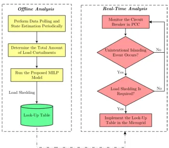
The general framework of the proposed load shedding algorithm is depicted in Fig. 1. In the first step, the

µG master controller (µGMC) gathers the network data

periodically (e.g., ∆T = 5 min.) and runs the state

estimation (SE) in order to obtain the proposed scheme’s

input parameters (operating point of the µG, load and

generation data, and µG topology). Then, the optimum

total amount of load curtailments is determined based

on the µG SFR model and the power exchange between

the µG and the upstream grid. Note that the obtained

total amount of load drops satisfies the µG dynamic and

static frequency limitations. The total amount of load shedding along with the SE data are fed into the proposed optimization model in order to arrange a look-up table including the location of load drops as well as appropriate post load shedding strategies. On the other side, the status of point of common coupling (PCC) circuit breaker is monitored using indication (i.e., binary) data. If an unintentional islanding happens and the amount of power mismatch is greater than a specific value, the pre-specified

load shedding scenarios will be implemented in the µG.

Detailed explanations about different parts of the proposed methodology are provided in the following sections.

Real-Time Analysis

Monitor the Circuit Breaker in PCC

Yes

Offline Analysis

Perform Data Polling and State Estimation Periodically

Determine the Total Amount of Load Curtailments

Run the Proposed MILP Model

Look-Up Table

Implement the Look-Up Table in the Microgrid Unintentional Islanding

Event Occurs? No

Load Shedding Load Shedding Is _Required?

Yes

No

Figure 1. The general framework of the proposed load shedding algorithm.

Time Frequency

Steady-State Frequency

Minimum Dynamic Frequency

Figure 2. A typical frequency response of a µG following an unintentional islanding event.

3. Optimal Amount and Threshold for

Acti-vation of Load Shedding

The aim of this section is to determine the minimum amount of load curtailments as well as a threshold for

activation of the load shedding process, while the µG

dynamic and steady-state frequency limitations are satis-fied. The minimum dynamic and steady-state frequencies

are indicated in a typical frequency response of a µG

following an unintentional islanding event, Fig. 2.

3.1. Frequency Response of the

µ

G to an

Island-ing Event

As the first step, the frequency response of the µG to

an islanding event should be specified. To do so, we use

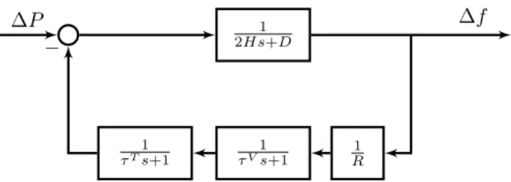
the aggregated SFR model of the µG as shown in Fig.

(4)

1 2Hs+D 1 τV_s₊₁ 1 τT_s₊₁ _R1 ∆P ∆f −

Figure 3. Block diagram of the adopted SFR model.

model of all DGs in the µG, where the frequency of the

center of inertia is considered by ignoring intermachine oscillations. The transfer function ₂_Hs1₊_D in the forward path represents the swing equation of the equivalent DG

as well as the effects of the µG loads which are lumped

into a single damping constant D. Moreover, the transfer

functions in the feedback loop are associated with the governor droop, governor time constant, and turbine time constant of the equivalent DG [13].

The transfer function of the adopted SFR model can be written as (1). H(s) = α1s 2₊_α 2s+α3 s3₊_β 1s2+β2s+β3 , (1) where α1= 1 2H, α2= 1 2H ₁ τT + 1 τV , α3= 1 2HτT_τV β1= D 2H + 1 τT + 1 τV, β2= 1 τT_τV + D 2H ₁ τT + 1 τV β3= 1 R+D 2HτT_τV .

3.2. Threshold for Activation of Load Shedding

Scheme

In the wake of an unintentional islanding, the

gover-nors and loads in the µG will respond to the incident,

thereby compensating for a portion of power mismatch. Consequently, load shedding is not necessary in all cases. Specifically, the minimum amount of power mismatch which would activate the load shedding process is obtained by (2).

P_thrM = minP_thr,SSFM , P_thr,DFM , (2)

where PM

thr,SSF and Pthr,DFM are the steady-state and

dynamic thresholds ofPM, respectively. Suppose that the

µG is not equipped with any load shedding scheme. In this

condition, if an unintentional islanding happens, the input power deviation of the SFR model in Fig. 3 is defined as (3).

∆P(t) =−PMu(t),∆P(s) =−P

M

s . (3)

Hence, the Laplace form of the frequency deviation func-tion is obtained as (4). ∆f(s) =H(s) ∆P(s) = F(s) z }| { α1s2+α2s+α3 s(s3₊_β 1s2+β2s+β3) −PM . (4)

Accordingly,F(s)can be decomposed into three terms

using partial-fraction decomposition as follows:

F(s) = α1s 2₊_α 2s+α3 s(s3₊_β 1s2+β2s+β3) =δ1 s + δ2 s−m1 + δ3s+δ4 s2₊_m 2s+m3 , (5) where m2= 2 3 β1− c1 2 − c2 2c1 , m3= 1 9 " β1− c1 2 − c2 2c1 2 +3 4 c1− c2 c1 2# , c1= 3 s c3+ p c2 3−4c32 2 , m1= −1 3 β1+c1+ c2 c1 , c2=β21−3β2, c3= 2β31−9β1β2+ 27β3, δ1= α3 β3 , δ2= α1m21+α2m1+α3 m3₁+m2m21+m3m1 , δ3=−(δ1+δ2), δ4= (δ1β2+δ2m3−α2)/m1.

Taking the inverse Laplace transform ofF(s),F(t)is given by: F(t) = δ1+δ2em1t+ δ3e −m2 2 t cos(φ) cos($t+φ) ! u(t), (6) where $= r m3− m2 2 4 , cosφ= $ r $2₊m2 2 − δ3 δ4 2 .

Therefore,∆f(t)can be written as (7).

∆f(t) =−PMF(t). (7)

3.2.1. Steady-State Threshold of PM_. _Given _∆_f₍_t₎_as

(7),∆fSSF (i.e., steady state frequency deviation) can be

computed as (8). ∆fSSF = lim

t→∞∆f(t) = −P M

δ1. (8)

The load shedding process will be triggered if the value

of ∆fSSF exceeds a given threshold∆fmax

SSF, that is: −PM δ1 ≥ |∆f_SSFmax|. (9)

(5)

Therefore, the minimum amount ofPM which violates the steady-state frequency limitation, and thus, triggers the load shedding process is acquired as follows:

PM ≥ |∆f_SSFmax| D+ 1 R . (10)

Accordingly, we define the right hand side of (10) as

the steady state threshold ofPM_.

3.2.2. Dynamic Threshold of PM_. _{The time when the}

frequency nadir happens (i.e., when the lowest frequency is reached before the frequency starts to recover) can be calculated by putting the first derivative of ∆f(t) equal to zero: tmin= min t:t >0,d∆f(t) dt = 0 . (11) Accordingly, the second trigger for the load shedding process is associated with the violation of nadir frequency limitation, that is:

|∆f(tmin)| ≥ |∆fDFmax|. (12)

The solution to this inequality in terms of PM, will

provide another criterion or lower bound (denoted by

P_thr,DFM in (2)) for the activation of the load shedding process.

3.3. Optimal Amount of Load Shedding

The minimum total amount of load curtailments satis-fying both steady-state and dynamic frequency limitations is calculated as (13).

pShed= max

pShed_SSF, pShed_DF , (13)

wherepShed

SSF andpShedDF are obtained as follows. Suppose

that the load shedding scheme is implemented in the µG

with a delay of tShed_{, subsequent to the unintentional}

islanding event. Accordingly, the input power deviation of the SFR model will be defined as (14).

∆P(t) =−PM_u₍_t_{) +}_pShed_{u t}₋_tShed

. (14)

Taking the Laplace transform of ∆P(t)yields

∆P(s) =1

s

−PM ₊_pShed_e−tShed_s

. (15) Hence, the Laplace form of the frequency deviation function is obtained as (16).

∆f(s) =F(s)−PM₊_pShed_e−tSheds_, ₍₁₆₎

where, F(s) is obtained from (5). Taking the inverse

Laplace transform of (16), ∆f(t) can be written as (17)

below

∆f(t) =−PM_F₍_t_{) +}_pShed_F _t₋_tShed

, (17) whereF(t)is calculated in (6).

3.3.1. Load Shedding Value Based on the Steady-State Frequency Limitation.Given∆f(t)as (17),∆fSSF can

be computed as (18) [8]. ∆fSSF = lim t→∞∆f(t) = −P M₊_pShed SSF δ1. (18)

Therefore, the minimum total amount of load shed-ding satisfying the steady-state frequency limitation (i.e.,

|∆fSSF| ≤ |∆fSSFmax|) is acquired as follows:

pShed_SSF =PM − |∆f_SSFmax| D+ 1 R . (19)

3.3.2. Load Shedding Value Based on the Dynamic Frequency Limitation.Similar to Section 3.2.2, the time when the frequency nadir happens is acquired by solving

(11), where ∆f(t) is calculated according to (17). By

applying the nadir frequency limitation (i.e., |∆fDF| ≤

|∆f_DFmax|), the minimum amount of load shedding

satisfy-ing dynamic frequency limitation (i.e.,pShed

DF ) is obtained.

It should be noted that the proposed method in this paper is aimed at bringing the frequency to the permissible range

(according to ∆fmax

SSF and ∆f

max

DF ) with the minimum

amount of load shedding. Obviously, the frequency should finally bring back to 60 Hz, but this transition can happen with a short delay (2-3 minutes) with the advantage of shedding fewer loads. Subsequent to load shedding, DERs will try to bring the frequency back to 60 Hz. If this cannot happen (e.g., due to some limitations in the output of DERs), further loads will be curtailed. This idea is consistent with the load-frequency control mechanisms which are done in three different successive steps (i.e., primary control, secondary control, tertiary control).

4. Optimization-Based

Load

Shedding

Scheme

4.1. Basic Model

In this section, the basic model of theµG load shedding

scheme is presented. The objective function and problem constraints are outlined as follows:

min X i∈ΩN X b∈Ω_Bi λV OLL_ib (1−xib)pDib (20) subject to X g:(g,i)∈MG pG_g + X r:(r,i)∈MRES pRES_r − X b∈Ω_Bi xibpDib = X (i,j)∈ΩL f₍P_i,j₎,∀i∈ΩN (21)

(6)

X g:(g,i)∈MG qG_g + X r:(r,i)∈MRES q_rRES− X b∈Ω_Bi xibq_ibD= X (i,j)∈ΩL f₍Q_i,j₎,∀i∈ΩN (22) f₍P_i,j₎=G(i,j) Vi2−ViVjcos(θi−θj) −B(i,j) ViVjsin(θi−θj),∀(i, j)∈ΩL (23) f₍Q_i,j₎=−B(i,j) V_i2−ViVjcos(θi−θj) −G(i,j) ViVjsin(θi−θj),∀(i, j)∈ΩL (24)

−f₍P,_i,jmax₎ ≤f₍P_i,j₎≤f₍P,_i,jmax₎ ,∀(i, j)∈ΩL (25)

−f₍Q,_i,jmax₎ ≤f₍Q_i,j₎≤f₍Q,_i,jmax₎ ,∀(i, j)∈ΩL (26)

f₍P_i,j₎+f₍P_j,i₎= G(i,j)

G2 (i,j)+B 2 (i,j) I(i,j) 2

≤f₍P,Loss,_i,j₎ max

= G(i,j) G2 (i,j)+B 2 (i,j) I max (i,j) 2 ,∀(i, j)∈ΩL (27)

V_imin≤Vi≤Vimax,∀i∈ΩN (28)

pD_ib =pD_ibκP I_ib (Vi/Vi∗) 2 +κP C_ib (Vi/V_i∗) +κ_ibP P,∀i∈ΩN, b∈ΩBi (29) qibD=q D ib κQI_ib (Vi/Vi∗) 2 +κQC_ib (Vi/V_i∗) +κ_ibQP,∀i∈ΩN, b∈ΩBi (30) −RgD≤p G g −p G,0 g ≤R U g,∀g∈ΩG (31) pG,_g min≤pG_g ≤pG,_g max,∀g∈ΩG (32) qG,_g min≤q_gG≤qG,_g max,∀g∈ΩG (33) X i∈ΩN X b∈Ω_Bi (1−xib)pD_ib ≥pShed (34) xib ∈ {0,1},∀i∈ΩN, b∈ΩBi. (35)

The objective function, (20), is the load shedding cost

in the µG, which should be minimized. λV OLL

ib is a

socioeconomic parameter and varies for different types of loads (e.g., industrial, commercial, agricultural, residential, and general loads). The group of equations (21)–(24) is related to the AC power flow equations. Line flow limits and bus voltage constraints are modeled through (25)– (27) and (28), respectively. Incorporation of a suitable

load model forµG loads plays an important role in power

system stability studies [9]. Therefore, the active and re-active power demands at different buses are modeled with voltage-dependent load model referred to as ZIP model, (29)–(30) [14]. Constraints (31)–(33) revolve around DG’s ramp-up and ramp-down limits (31) and active and reactive power generation limits of DGs (32)–(33). The minimum total load shedding constraint is expressed as (34), and finally, the status of loads is characterized by a binary variable in (35).

4.2. Linearization of the Basic Model

The developed problem in Section 4.1 is a mixed-integer nonlinear programming (MINLP) model. In order to attain computational efficiency, the nonlinear equations ought to

be linearized. The nonlinear terms xibpD

ib and xibqibD in

(21)–(22) and (34) are the product of a binary and continu-ous variables. We can linearize these terms with the big-M method by introducing auxiliary semi-continuous variables (i.e., αP ib ∆ = xibpD ib and α Q ib ∆ = xibqD

ib) and the set of

equations (36)–(39). In order to reduce the integrality gap in the linearized version of the aforementioned constraints, Big-Ms (i.e.,MibandM_ib0 ) should be as small as possible, and it is usually challenging to determine correct values for them to use for each specific implementation. However,

in this particular application, we can set Mib =pD_ib and

M_ib0 =qD_ib,∀i∈ΩN, b∈ΩBi. Note that these data (i.e.,

the upper bounds of active and reactive loads) are usually available in any system.

Moreover, considering reasonable assumptions given in Table 1 [15], AC power flow equations are replaced by their piecewise linear approximation form as (40)–(49). Finally, considering the permissible range for bus voltage magnitudes at different buses (i.e., 0.9 ≤ Vi, Vi∗ ≤ 1.1),

(29)–(30) can be reasonably approximated by (50)–(51) [9]. With these changes, the proposed model is trans-formed into an MILP model.

−(1−xib)Mib≤αPib−p D ib

≤Mib(1−xib),∀i∈ΩN, b∈ΩBi

(36)

(7)

Table 1. Constituent Terms in the Linearized Power Flow Equations [15]

Term Approximation Max. Abs. Error

V2 i 2Vi−1 0.0025 ViVjcos(θi−θj) Vi+Vj+cos(θi−θj)−2 0.0253 ViVjsin(θi−θj) sin(θi−θj) 0.0659 sin(θi−θj) θi−θj 0.0553 −(1−xib)M_ib0 ≤αQ_ib−qD_ib ≤M_ib0 (1−xib),∀i∈ΩN, b∈ΩBi (38)

−xibM_ib0 ≤αQ_ib≤M_ib0 xib,∀i∈ΩN, b∈ΩBi (39)

f₍P_i,j₎=G(i,j) Vi−Vj−ω(i,j)+ 1

−B(i,j)(θi−θj),∀(i, j)∈ΩL

(40)

f₍Q_i,j₎=−B(i,j) Vi−Vj−ω(i,j)+ 1 −G(i,j)(θi−θj),∀(i, j)∈ΩL (41) ω(i,j)= X p∈ΩP s(i,j)pCpB,∀(i, j)∈ΩL (42) θi−θj= X p∈ΩP s(i,j)pBBp,∀(i, j)∈ΩL (43) X p∈ΩP s(i,j)p= 1,∀(i, j)∈ΩL (44) X p∈ΩP v(i,j)p= 1,∀(i, j)∈ΩL (45) s(i,j)p1 ≤v(i,j)p1,∀(i, j)∈ΩL (46)

s(i,j)p≤v(i,j)p−v(i,j)(p−1),

∀(i, j)∈ΩL, p∈ΩP, p6={p1, pn} (47) s(i,j)pn≤v(i,j)(pn−1),∀(i, j)∈ΩL (48) v(i,j)pn= 0,∀(i, j)∈ΩL (49) pD_ib =pD_ib κP I_ib 1 + 2 (Vi−V_i∗) +κP C_ib (Vi/Vi∗) +κ P P ib ,∀i∈ΩN, b∈ΩBi (50) q_ibD=qD_ib κQI_ib 1 + 2 (Vi−Vi∗) +κQC_ib (Vi/Vi∗) +κ QP ib ,∀i∈ΩN, b∈ΩBi. (51)

Table 2. Technical Data of DG Units

Parameter Unit DG1 DG2 DG3 DG4 pDG,min (MW) 1 1 1 1 pDG,max _(MW) ₄ ₃_.₃₈ ₃_.₃₈ ₄_.₇₂ qDG,min_(MW) ₋₀_.₅ ₋₀_.₅ ₋₀_.₅ ₋₀_.₅ qDG,max_(MW) ₂ ₂ ₂ ₂ RU_(MW/min.) ₂_.₄ ₂_.₄ ₂_.₄ ₂_.₄ RD _(MW/min.) ₂_.₄ ₂_.₄ ₂_.₄ ₂_.₄

Table 3. µG Dynamic Data [5], [18]

Parameter Value Parameter Value

H (sec.) 2 τV _(sec.) ₀_.₁

D 1 τT (sec.) 0.5

R 0.05 tShed_(msec.) ₁₀₀

∆f_SSFmax (Hz) 0.2 ∆f_DFmax(Hz) 0.5

5. Case Study and Performance Evaluation

5.1. System Model and Parameters

In this section, the performance of the proposed scheme

for theµG load shedding problem is thoroughly evaluated

using a large-scale µG. All simulations were conducted

on a PC with Intel CoreTMi5 CPU @2.67 GHz and 4

GB RAM. The optimization model was implemented in

the GAMSR IDE environment. The MILP and MINLP

models were solved with IBM ILOG CPLEXR and

BON-MIN solvers, respectively. The modified IEEE 33-bus test system, which is a radial medium voltage (i.e., 12.66 kV)

distribution system, is used as the test µG in this paper.

The system topology and components are depicted in Fig. 4 and the feeders and loads’ data are obtained from [16]

and [17]. The testµG includes three DGs, whose technical

data are given in Table 2. Meanwhile, three wind turbines as RESs with a total capacity of 3 MW are installed at buses 14, 16, and 31. To have a more realistic study, the

load at each node of the µG is divided into three load

blocks. Furthermore, five different load types (i.e., general, residential, agricultural, commercial, and industrial) with different VOLLs are taken into account, Fig. 5 [9]. Finally, the test system’s dynamic data can be found in Table 3.

5.2. Simulated Cases and Discussion

In this section, three different contingencies are sim-ulated in the test system, Table 4. To evaluate the per-formance of the proposed methodology, it is compared with the conventional UFLS scheme. The amount and setting of conventional UFLS relays have been designed according to [19]. The simulation results are summarized in the following figures and tables. According to Fig. 6, the

(8)

1

Abstract—

I. CASE STUDY AND PERFORMANCE EVALUATION

In this section, the performance of the proposed scheme for the µG load shedding problem is thoroughly evaluated using a large-scale µG. All simulations were conducted on a PC with Intel CoreTM i7 CPU @3.20 GHz and 4 GB RAM. The MILP optimization model was implemented in the GAMS®IDE environment [**] and the model was solved with IBM ILOG CPLEX ® 12.4 solver [***].

The modified IEEE 33-bus test system is a medium voltage (i.e., 12.66 kV) distribution network which is used as the test µG in this paper. The µG topology and components are depicted in Fig. 4 and the feeders’ data are obtained from [***]. Note that the switchable lines are also depicted in this figure by red dashed trajectories. The location and size of DGs are determined according to [***]. The technical characteristics of the DGs can be found in Tables II.

Three RESs with a total capacity of 3 MW are installed at buses 14, 16, and 31. As µG buses are located in a small geographical region, the outputs of the three RESs are considered to be the same in our study.

Fig. 4. Single line diagram of the simulated µG.

Adoption of a reasonable model for representing the load behavior plays a prominent role in both voltage and frequency stability analyses. To have a more realistic study, the load at

each node of the µG is divided into three load blocks. Moreover, five different load types (including general, residential, agricultural, commercial, and industrial) are taken into account. The contribution percentage as well as the VOLL of these loads are provided in Table III.

TABLE II

TECHNICAL CHARACTERISTICS OF DEPLOYED CONVENTIONAL DGS Unit Technical Constraints

(MW) G i P G (MW) i P G (MVAr) i Q G (MW) i Q R H DG1 3 0.21 2.1 -2.1 2 2 DG2 2 0.19 1.9 -1.9 2 2 DG3 2 0.19 1.9 -1.9 2 2 DG4 3 0.22 2.2 -2.2 2 2 TABLE I

VOLL FOR VARIOUS LOAD TYPES [22]

Load Type VOLL ($/MW) Contribution Percentage (%)

General 650 16.4

Residential 190 6

Agricultural 420 23.5

Commercial 4365 11.6

Industrial 5172 42.5

A. Results and Discussion

Considering a mipgap of 0%, the computation time was 20 seconds which further illustrates the practical merits of the proposed framework in case of real-scale networks.

Simulation and results

Amin Gholami, Student Member, IEEE, Tohid Shekari, StudentMember, IEEE, Farrokh Aminifar,

SeniorMember, IEEE, and Mohammad Shahidehpour, Fellow, IEEE

Upstream Network MG Operator 1 2 3 4 5 6 7 8 9 10 11 19 18 17 16 15 14 13 12 20 21 22 33 32 31 30 29 28 27 26 23 24 25 PCC Substation DG4 RES1 RES3 DG3 RES2 DG1 DG2

Figure 4. Single line diagram of the simulatedµG [17].

3

General Residential Agricultural Commercial Industrial

0 1000 2000 3000 4000 5000 6000 V O L L ( $ /M W )

General Residential Agricultural Commercial Industrial

0 1000 2000 3000 4000 5000 6000 V O L L ( $ /M W )

Figure 5. VOLL for different types of loads.

amount of load shedding in the proposed method is less than that of the conventional UFLS approach. Considering the SFR model in the developed approach is the main reason of this observation. Similarly, the load shedding cost associated with the proposed method is much less than that of the conventional UFLS approach, Fig. 7. The reason is that in the conventional case, the locations of candidate loads to be shed are fixed, despite the fact that the VOLL of different feeders changes during the day. Therefore, in the conventional case, the interruption cost of dropped loads is not optimum around-the-clock. It is worth mentioning that in the proposed method, although the loads are shed according to their VOLL, operational limitations play a more important role. Indeed, the model is implemented in such a way that the load shedding cost is minimized, and at the same time, the network operational limitations are preserved.

As can be seen in Fig. 8, for all unintentional islanding

events, minimum frequency of the µG is greater in the

proposed approach due to its high speed in event indication and implementing the load shedding scenario. Taking a glance at Fig. 9 yields that the steady-state frequency

of the µG following all contingencies is higher for the

conventional UFLS method. On the other hand, the steady-state frequency associated with the proposed scheme is still in the safe range. Therefore, it can be inferred that the

Table 4. Simulated Contingencies

Contingency No. PM _(MW) _pShed

SSF p Shed DF 1 3 1.81 1.7 2 4 2.81 2.86 3 5 3.81 4.15 1 Abstract— In this section, L oa d S h ed d in g ( M W ) C o s t ($ )

the performance of the proposed scheme for the µG load shedding problem is thoroughly evaluated using a large-scale µG. All simulations were conducted on a PC with Intel CoreTM i7 CPU @3.20 GHz and 4 GB RAM. The MILP optimization model was implemented in the GAMS®IDE environment [**] and the model was solved with IBM ILOG CPLEX ® 12.4 solver [***].

The modified IEEE 33-bus test system is a medium voltage (i.e., 12.66 kV) distribution network which is used as the test µG in this paper. The µG topology and components are depicted in Fig. 4 and the feeders’ data are obtained from [***]. Note that the switchable lines are also depicted in this figure by red dashed trajectories. The location and size of DGs

are determined according to [***]. The technical

characteristics of the DGs can be found in Tables II.

Adoption of a reasonable model for representing the load behavior plays a prominent role in both voltage and frequency stability analyses. To have a more realistic study, the load at each node of the µG is divided into three load blocks. Moreover, five different load types (including general,

NES imulation and results

Figure 6. Comparison between the proposed and conventional UFLS methods in terms of load shed-ding. 1 Abstract— In this section, L oa d S h ed d in g ( M W ) C o s t ($ )

NES imulation and results

Figure 7. Comparison between the proposed and conventional UFLS methods in terms of load shedding cost.

conventional method sheds non-optimal amount of loads encountering different events. These results prove that the proposed method is capable of preserving the system from collapsing and moving it to a new steady state and stable condition.

It is worth mentioning that keeping the bus voltages and line flows within the permissible range would

guar-antee a secure µG operation following the load shedding

process. Therefore, if these constraints are violated in the network, the proposed methodology seeks to return them to the permissible range by modifying the available control variables.

Table 5 provides the curtailed load blocks in contin-gency 2 for both the nonlinear and linear optimization models, where differences are highlighted in red bold. In this contingency, the optimal values of the objective function for the nonlinear and linear models are $623.4 and $625.6, respectively. Accordingly, the load shedding costs are roughly equal in these two models, and the curtailed loads are identical in most cases. Moreover, Table 6 shows a comparison between the computation time of the two models, which has been obtained using a relative

(9)

1 Abstract— In this section, L oa d S h ed d in g ( M W ) C o s t ($ )

NES imulation and results

Figure 8. Comparison between the proposed and conventional UFLS methods in terms of minimum dynamic frequency. 1 Abstract— In this section, L oa d S h ed d in g ( M W ) C o s t ($ )

NES imulation and results

Figure 9. Comparison between the proposed and conventional UFLS methods in terms of steady-state frequency.

optimality criterion (i.e., Optcr) of10−2. As can be seen, the computation time is considerably diminished in the linear model, and this is highly effective in precarious situations such as the load shedding process, since prompt measures can keep electromechanical dynamics away from becoming stability threatening.

6. Conclusion

The proliferation of µGs all over the world has been

remarkable in recent years, and their growth prospects in

the future are astounding. µGs can improve the resilience

of the grid based on their self-supply and island-mode

capabilities. However, when a µG unintentionally enters

the island mode, a considerable number of customers (or even all of them) are disconnected from the grid in order to maintain the load-generation equilibrium. New methodologies are therefore required to optimize the load

shedding process in µGs. In this paper, an

optimization-based load shedding model is presented as a promising tool to attain this goal. Mathematically, the load shedding model is formulated as a MILP problem. The structure of the proposed scheme reduces its communication require-ments which is a major challenge in practice. The most relevant aspects of the proposed load shedding scheme are illustrated using a large-scale case study based on a 33-bus

µG. It was observed that the proposed method sheds less

amount of load in comparison with the conventional UFLS

Table 5. Comparison Between the Linear and Nonlinear Load Shedding Optimization Models

1

Abstract_—

I. CASE STUDY AND PERFORMANCE EVALUATION

This is the table

Nonlinear Model Linear Model

Load Block # Load Block #

Bus # B1 B2 B3 B1 B2 B3 2 1.06 1.06 3 0.96 0.96 5 0.65 0.65 6 0.63 7 2.22 10 0.70 0.69 0.70 0.68 11 0.51 12 0.67 0.67 15 0.75 0.71 0.74 16 0.68 0.74 0.67 17 0.69 0.68 18 1.03 20 0.95 0.95 0.95 0.95 21 0.95 0.95 22 0.95 0.94 24 4.62 4.61 25 4.72 4.72 28 0.66 0.66 30 2.16 2.16 32 2.42 33 0.67 0.66 0.70 0.67 0.69

that the switchable lines are also depicted in this figure by red dashed trajectories. The location and size of DGs are determined according to [***]. The technical characteristics of the DGs can be found in Tables II.

of the proposed scheme for the µG load shedding problem is thoroughly evaluated using a large-scale µG. All simulations were conducted on a PC with Intel CoreTM i7 CPU @3.20 GHz and 4 GB RAM. The MILP optimization model was implemented in the GAMS®IDE environment [**] and the model was solved with IBM ILOG CPLEX ® 12.4 solver [***].

Adoption of a reasonable model for representing the load behavior plays a prominent role in both voltage and frequency

Lost Load Table

Table 6. Computation Time of the Linear and Nonlinear Models

Contingency No. Nonlinear model Linear model

1 93sec. 9sec.

2 214sec. 7sec.

3 40sec. 7sec.

approach. Meanwhile, the developed structure outper-formed the conventional scheme in terms of load shedding cost and minimum dynamic frequency following the load shedding process. Future studies could reformulate power flow equations for radial systems (since the complex power flow equations presented in this paper are not necessary for radial networks). Moreover, an unbalanced power flow model can be adopted to make the proposed load shedding method more practical in real world applications.

References

[1] J. A. Momoh, S. Meliopoulos, and R. Saint, “Centralized and distributed generated power systems-a comparison ap-proach,”Future grid initiative white paper, PSERC, pp. 1– 33, 2012.

[2] D. T. Ton and M. A. Smith, “The U.S. Department of En-ergy’s microgrid initiative,”The Electricity Journal, vol. 25, no. 8, pp. 84–94, 2012.

(10)

[3] Recommended Practice for Utility Interconnected Photo-voltaic (PV) Systems, IEEE Std. 929-2000, 2000. [4] IEEE Standard for Interconnecting Distributed Resources

Into Electric Power Systems, IEEE Std. 1547TM, Jun. 2003. [5] P. Mahat, Z. Chen, and B. Bak-Jensen, “Under frequency load shedding for an islanded distribution system with distributed generators,” IEEE Trans. Power Del., vol. 25, no. 2, pp. 911–918, Apr. 2010.

[6] H. Seyedi and M. Sanaye-Pasand, “New centralized adap-tive load shedding algorithms to mitigate power system blackouts,”IET Gener. Transm. Distrib., vol. 3, no. 1, pp. 99–114, Jan. 2009.

[7] J. Tang, J. Liu, F. Ponci, and A. Monti, “Adaptive load shedding based on combined frequency and voltage stabil-ity assessment using synchrophasor measurements,”IEEE Trans. Power Syst., vol. 28, no. 2, pp. 2035–2047, May 2013.

[8] T. Shekari, F. Aminifar, and M. Sanaye-Pasand, “An ana-lytical adaptive load shedding scheme against severe com-binational disturbances,”IEEE Trans. Power Syst., vol. 31, no. 5, pp. 4135–4143, Sept. 2016.

[9] T. Shekari, A. Gholami, F. Aminifar, and M. Sanaye-Pasand, “An adaptive wide-area load shedding scheme incorporating power system real-time limitations,” IEEE Syst. J., to be published.

[10] U. Rudez and R. Mihalic, “Wams-based under frequency load shedding with short-term frequency prediction,”IEEE Trans. Power Del., vol. 31, no. 4, pp. 1912–1920, Aug. 2016.

[11] V. V. Terzija, “Adaptive underfrequency load shedding based on the magnitude of the disturbance estimation,” IEEE Trans. Power Syst., vol. 21, no. 3, pp. 1260–1266, Aug. 2006.

[12] Y. Lu, W. Kao, and Y. Chen, “Study of applying load shedding scheme with dynamic d-factor values of various dynamic load models to taiwan power system,”IEEE Trans. Power Syst., vol. 20, no. 4, pp. 1976–1984, Nov. 2005. [13] P. Kundur,Power system stability and control. McGraw–

hill, New York, 1994.

[14] IEEE Task Force on Load Representation for Dynamic Performance, “Bibliography on load models for power flow and dynamic performance simulation,”IEEE Trans. Power Syst., vol. 10, no. 1, pp. 523–538, Feb. 1995.

[15] P. A. Trodden, W. A. Bukhsh, A. Grothey, and K. I. McK-innon, “Optimization-based islanding of power networks using piecewise linear ac power flow,”IEEE Trans. Power Syst., vol. 29, no. 3, pp. 1212–1220, May 2014.

[16] M. E. Baran and F. Wu, “Network reconfiguration in distribution system for loss reduction and load balancing,” IEEE Trans. Power Del., vol. 4, no. 2, pp. 1401–1407, Apr. 1989.

[17] A. Gholami, T. Shekari, F. Aminifar, and M. Shahideh-pour, “Microgrid scheduling with uncertainty: the quest for resilience,”IEEE Trans. Smart Grid, vol. 7, no. 6, pp. 2849– 2858, Nov. 2016.

[18] A. Mokari-Bolhasan, H. Seyedi, B. Mohammadi-ivatloo, S. Abapour, and S. Ghasemzadeh, “Modified centralized ROCOF based load shedding scheme in an islanded distri-bution network,”Int. J. Elec. Power & Energy Syst., vol. 62, pp. 806–815, Nov. 2014.

[19] M. Abedini, M. Sanaye-Pasand, and S. Azizi, “Adaptive load shedding scheme to preserve the power system sta-bility following large disturbances,” IET Gen. Transm. Distrib., vol. 8, no. 12, pp. 2124–2133, Dec. 2014.