Markus K. Brunnermeier and Martin Oehmke
Predatory short selling
Article (Accepted version)
(Refereed)
Original citation:
Brunnermeier, Markus K. and Oehmke (2013). Predatory short selling
Review of Finance
18, (3) pp. 2153-2195. ISSN 1572-3097
DOI:
10.1093/rof/rft043
© 2013
Oxford University Press
This version available at: http://eprints.lse.ac.uk/84517/
Available in LSE Research Online: October 2017
LSE has developed LSE Research Online so that users may access research output of the
School. Copyright © and Moral Rights for the papers on this site are retained by the individual
authors and/or other copyright owners. Users may download and/or print one copy of any
article(s) in LSE Research Online to facilitate their private study or for non-commercial research.
You may not engage in further distribution of the material or use it for any profit-making activities
or any commercial gain. You may freely distribute the URL (http://eprints.lse.ac.uk) of the LSE
Research Online website.
This document is the author’s final accepted version of the journal article. There may be
differences between this version and the published version. You are advised to consult the
publisher’s version if you wish to cite from it.
Markus K. Brunnermeier
1and Martin Oehmke
21Princeton University, NBER, and CEPR;2Columbia University
Abstract. Financial institutions may be vulnerable to predatory short selling. When the stock of a financial institution is shorted aggressively, leverage constraints imposed by short-term creditors can force the institution to liquidate long-term investments at fire sale prices. For financial institutions that are sufficiently close to their leverage constraints, predatory short selling equilibria co-exist with no-liquidation equilibria (thevulnerability
region), or may even be the unique equilibrium outcome (thedoomed region). Increased
coordination among short sellers expands the doomed region, where liquidation is the unique equilibrium. Our model provides a potential justification for temporary restrictions of short selling for vulnerable institutions and can be used to assess recent empirical evidence on short-sale bans.
JEL Classification: G01, G20, G21, G23, G28
For helpful comments, we thank Thierry Foucault (the editor), an anonymous referee, Charles Jones, Marco Pagano, Alejandro van der Ghote, and seminar participants at Columbia University.
1. Introduction
The financial crisis of 2007-09 and the recent European sovereign debt crisis have led to a heated discussion on short selling financial stocks. For example, as financial stocks fell sharply in the spring, summer, and fall of 2008, a number of banks, most notably Bear Stearns, Lehman Brothers, and Morgan Stanley, blamed short sellers for their woes.1 In response, the Securities and Exchange Commission (SEC) and a number of international financial regulators took measures against short selling; most significantly, some imposed temporary restrictions on the short selling of financial stocks, some even on short selling in general. In August 2011, when European banks were struggling because of losses due to the European sovereign debt crisis, market regulators in France, Spain, Italy and Belgium imposed temporary bans on short selling for some financial stocks.
On both occasions, the worry was that short selling was “predatory,” in the sense that short sellers were attempting to bring down fundamentally solvent financial institutions by triggering self-fulfilling downward spirals. However, this line of argument is at odds with the consensus view in economics, which—broadly speaking—says that there is nothing wrong with short selling. In fact, most economists would argue that short selling is a valuable activity—short sellers help enforce the law of one price, facilitate price discovery, and enhance liquidity. Moreover, short sale restrictions may lead to overvaluation and bubbles, and reduce the ability of investors to hedge exposures.2 In the light of these findings, is there any economic justification to impose restrictions on short selling the stock of financial institutions?
In this paper, we present a model of predatory short selling. We show that, even though short selling activity is beneficial during “normal times,” at times of stress short sellers can, in fact, destabilize financial institutions through predatory short sales. Predatory short selling can occur in our model because financial institutions are subject to leverage constraints imposed by their short-term creditors and uninsured depositors. These lever-age constraints capture a first-order difference between financial institutions and regular corporates: Relative to corporations that can match maturities of assets and liabilities, the business model of a financial institution almost necessarily involves maturity and liquidity mismatch (see, e.g., Diamond and Dybvig (1983) and Brunnermeier, Gorton, and Krish-namurthy (2013)), which exposes financial institutions to sudden withdrawal of funding in response declines in equity value. We show that, in the presence of such leverage con-straints, predatory short sellers that temporarily depress the stock price of a financial 1 See, for example, “Anatomy of the Morgan Stanley Panic,”Wall Street Journal, Novem-ber 24, 2008.
2 For theoretical models on how short-sale constraints can lead to overvaluation, specu-lative trading, and bubbles, see, for example, Miller (1977), Harrison and Kreps (1978), Scheinkman and Xiong (2003), and Hong and Stein (2003). Diamond and Verrecchia (1987) show theoretically that a market with short-sale constraints incorporates information more slowly than a market in which short sales are not restricted. Empirical evidence that short sellers contribute to market efficiency and market quality can be found, among others, in Dechow, Hutton, Meulbroek, and Sloan (2001), Desai, Krishnamurthy, and Kumar (2006), Bris, Goetzmann, and Zhu (2007) , Chang, Cheng, and Yu (2007), Boehmer, Jones, and Zhang (2008), Saffi and Sigurdsson (2011), and Boehmer and Wu (2013). Short positions are important hedging tools in a number of common trading strategies (e.g., hedging options, convertible bonds, or market risk in long-short strategies).
institution can force the financial institution to sell long-term assets in order to repay debt to satisfy their leverage constraint. When long-term assets have to be unwound at a sufficient discount, the resulting losses for the financial institution allow predatory short sellers to break even on their short positions.
Our model implies that financial institutions can be vulnerable to attacks from preda-tory short sellers when their balance sheets are weak. For financial institutions that are sufficiently close to their leverage constraints, predatory short selling equilibria co-exist with no-liquidation equilibria (the vulnerability region), or may even be the unique equi-librium outcome (the doomed region). In the vulnerability region there are two stable equilibria. In one equilibrium, no predatory short selling occurs. In that case, the financial institution does not violate its constraint and can hold its long-term investments until maturity. In the second equilibrium, however, predatory short selling causes the financial institution to violate its leverage constraint, leading to a complete liquidation of its long-term asset holdings. In the doomed region, there is a unique stable equilibrium in which predatory short sellers force the financial institution to liquidate its entire long-term asset holdings.
Comparing a regime with short selling to one with short-sale restrictions shows that, during “normal times” when financial institutions are well capitalized, the fundamental value of the financial institution cannot be affected by the presence of predatory short sell-ers. In this region short sellers exclusively fulfill their beneficial roles of providing liquidity and preventing overvaluation and bubbles that may distort real investment decisions— confirming the consensus view that restricting short selling during normal times is likely to have undesired consequences. However, this changes once a financial institution enters the vulnerability region or the doomed region. Here, short sellers can force inefficient liqui-dation of the financial institutions’ long-term assets, such that restrictions on short selling can potentially be welfare-enhancing.
By highlighting the possibility of multiple equilibria, our model underlines the impor-tant role of coordination in short selling attacks. Specifically, adding a large short seller (or, equivalently, a mass of small short sellers that can coordinate their actions) to our competitive benchmark model expands the doomed region, where a predatory short selling attack and full liquidation is the unique (and inefficient) outcome. This contrasts sharply with the situation where sellers are regular shareholders (rather than short sellers): In this case, adding a large shareholder (or a mass of coordinated small shareholders) increases the safety region, in which no liquidation is the unique equilibrium. Finally, we show that when there is a large short seller and a potential large support buyer, the doomed region depends on the relative strength (or ability to coordinate) of the large short seller and the support buyer.
Overall, our results provide a potential justification for temporary short sale restrictions for financial institutions at times when their balance sheets are weak. These restrictions should be temporary and targeted specifically at weak financial institutions because well-capitalized financial institutions are not susceptible to predatory short selling attacks, such that the only effect of a ban on short selling for those institutions would be a reduction in liquidity and market quality of their stock. Moreover, because our results are driven by a constraint on market leverage that is imposed by short-term creditors, it highlights the particular vulnerability of financial institutions—because of the maturity mismatch and liquidity mismatch inherent in their business models, financial institutions are subject to financial fragility in the form of creditor runs, which makes them vulnerable to predatory short sellers. Our model is less likely to apply to firms with more stable capital structures.
Finally, our analysis has implications on the disclosure of short positions. By facilitating coordination among short sellers, full and timely disclosure of short positions may in fact make iteasier for short sellers to prey on vulnerable financial institutions.
The empirical evidence on the recent short-sale bans in the U.S. and Europe unambigu-ously documents reductions in market liquidity and market quality as a result of short sale bans. However, there is no strong empirical support for positive price effects of recent short sale bans, perhaps the main motivation of these bans. Using daily international data on recent short-sale bans around the world, Beber and Pagano (2013) document that the short-sale bans implemented during the financial crisis of 2007-2009 led to reductions in market liquidity and slower price discovery. They also document that short-sale constraints failed to support stock prices, except potentially those of large U.S. financial stocks. In similar spirit, Boehmer, Jones, and Zhang (2013), using intraday data on the 2008 short-sale ban in the U.S., document a deterioration of liquidity and market quality in response to the short-sale ban. Yet, their analysis also finds little evidence that short-sale bans sup-ported prices: Only the largest financial institutions had (permanent) positive abnormal returns during 2008 short-sale ban, and Boehmer, Jones, and Zhang (2013) point out that the price effects of the short selling ban are hard to disentangle from the effects of the contemporaneous Troubled Asset Relief Program (TARP).3
Our results may help interpret the existing empirical findings on the effect of short selling bans, and may also be useful in the empirical design of future studies. First, when looking at price effects, our model suggests that financial institutions, rather than regular firms, should be particularly affected by short sale bans. Second, in our model, the ability of short sellers to prey on financial institutions depends crucially on the financial condition of the financial institution. Hence, a second cross-sectional prediction of our model is that in assessing the price effects of short-sale restrictions, one should control for leverage, liquidity mismatch, or similar variables that measure financial fragility. The prediction of our model is that it is vulnerable financial firms for which the price effects of short sale bans are likely largest. Third, our model highlights the importance of taking into account the potential multiplicity of equilibria when interpreting the empirical evidence. For example, if investors expect that, with some probability, there is a switch to the dominated equilibrium in which the bank goes bankrupt, the elimination of the bad equilibrium through temporary short selling bans when financial institutions enter the vulnerability region may lead to permanent positive price effects. In addition to the cross-sectional predictions above, a 3 A number of other studies have investigated the effects of recent short-sale bans. For example, Marsh and Payne (2012) document a decrease in market quality in UK equity markets in response to the 2008 short selling ban. Using U.S. and European data, Lioui (2011) documents an increase in volatility in response to the 2008 short selling ban, but no effect on the price skewness. Autore, Billingsley, and Kovacs (2011) document that during the 2008 short sale ban in the U.S., stocks with a larger decline in liquidity also have poorer contemporaneous returns, consistent with the model of Amihud and Mendelson (1986). Harris, Namvar, and Phillips (2013) use a factor model to document price inflation in banned stocks as a result of the 2008 short selling ban in the U.S., particularly for firms without traded options. Their results suggest that price effects were temporary for stocks with negative pre-ban performance and permanent for firms with positive pre-ban performance. Kolasinski, Reed, and Thornock (2013) document that variations in short interest had larger price effect during the shorting ban, consistent with an increase in the informativeness of short sales in response to increased short sale restrictions.
novel prediction of our model is that the vulnerability of a financial institution to predatory short selling depends not only on its own balance sheet but also on the balance sheets (or funding conditions) of its large shareholders.
At a theoretical level, the potential justification for restrictions on short selling provided by our model is similar to that given in the literature on feedback effects from stock prices to firms’ real decisions.4 For example, Goldstein and G¨umbel (2008) provide an asymmetric information model, in which a feedback loop to real investment decisions allows a short seller to make a profit even in the absence of fundamental information. Khanna and Mathews (2012) study the interaction between an uninformed speculator and an informed blockholder to a firm. They show that, under certain conditions, manipulation by an uninformed speculator is possible even in the presence of an informed blockholder, whose incentives are aligned with value maximization. A major difference between these papers and our analysis is the channel through which short selling can be profitable. In both Goldstein and G¨umbel (2008) and Khanna and Mathews (2012), short sellers reduce price informativeness, thereby inducing the firm (whose manager learns from prices) to inefficiently distort its (future) investments, which makes the short position profitable. In our framework, price declines brought about by short sellers can trigger inefficient early liquidation of existing investments via the leverage constraint. In our view, this latter channel is particularly relevant for the recent discussion on short-sale bans, which has centered around financial institutions.A related feedback mechanism arises in Goldstein, Ozdenoren, and Yuan (2013). In their model, a provider of equity capital learns from the firm’s stock price and provides less capital to the firm when he infers negative information from the firm’s stock price.5
In terms of the focus on financial institutions, the paper closest to ours is Liu (2011). Liu develops a two-stage global games model: In the first stage, short sellers take positions. In the second stage, creditors decide whether or not to roll over their debt. As in Goldstein and G¨umbel (2008), the presence of short sellers reduces price informativeness. The resulting increase in uncertainty about fundamentals reduces the value of short-term debt claims (due to their concave payoff) and can induce creditors to run in the second stage. Hence, a major difference to our paper is how short-sale attacks work: In our framework it is the reduction in the market value of equity that makes a short selling attack possible. In Liu (2011), it is the increase in price uncertainty (and not the price reduction) that leads to a creditor run. Liu’s framework leads to policy prescriptions that are broadly in line with ours. First, as in our model, his framework implies that banks with weak fundamentals are prone to short-sale attacks. Second, Liu argues that more maturity mismatch makes short-selling attacks more likely. This is consistent with our model, where one can interpret the severity of the leverage constraint as a proxy for maturity mismatch (the more short term creditors the bank has, the more binding the run constraint).6
4 For a comprehensive survey of this literature, see Bond, Edmans, and Golstein (2012). 5 Khanna and Sonti (2004) and Ozdenoren and Yuan (2008) provide models with exoge-nous feedback from financial markets to real outcomes.
6 More broadly, our paper also relates to the literature on market manipulation, and predatory trading. Allen and Gale (1992) provide a model in which a non-informed trader can make a profit if investors think the manipulator may be an informed trader. Other papers that consider manipulative trading strategies include Allen and Gorton (1992), Benabou and Laroque (1992), Kumar and Seppi (1992), Gerard and Nanda (1993), Chakraborty and Yilmaz (2004), and Brunnermeier (2005). Brunnermeier and Pedersen
The remainder of the paper is structured as follows. Section 2. gives a brief summary of regulatory response to short selling during the financial crises of 2007-2009 and the European sovereign debt crisis of 2011. Section 3. presents the model. Section 4. pro-vides a discussion of the model’s policy implications and empirical predictions. Section 5. concludes. All proofs are in the Appendix.
2. Recent regulatory response to short selling
As a result of the financial market turmoil in 2008, the SEC and a number of international financial market regulators put in effect a number of new rules regarding short selling. In July the SEC issued an emergency order banning so-called “naked” short selling7 in the securities of Fannie Mae, Freddie Mac, and primary dealers at commercial and investment banks. In total 18 stocks were included in the ban, which took effect on Monday July 21 and was in effect until August 12.
On September 19 2008, the SEC bannedallshort selling of stocks of financial companies. This much broader ban initially included a total of 799 firms, and more firms were added to this list over time. In a statement regarding the ban, SEC Chairman Christopher Cox said, “The Commission is committed to using every weapon in its arsenal to combat market manipulation that threatens investors and capital markets. The emergency order temporarily banning short selling of financial stocks will restore equilibrium to markets. This action, which would not be necessary in a well-functioning market, is temporary in nature and part of the comprehensive set of steps being taken by the Federal Reserve, the Treasury, and the Congress.” This broad ban of all short selling in financial institutions was initially set to expire on October 2, but was extended until Wednesday October 9, i.e., three days after the emergency legislation (the bailout package) was passed.
In addition to measures taken by the SEC, a number of international financial regulators also acted in response to short selling. On September 21 2008, Australia temporarily banned all forms of short selling, with only market makers in options markets allowed to take covered short positions to hedge. In Great Britain, the Financial Services Authority (FSA) enacted a moratorium on short selling of 29 financial institutions from September 18 2008 until January 16 2009. Also Germany, Ireland, Switzerland and Canada banned short selling of some financial stocks, while France, the Netherlands and Belgium banned naked short selling of financial companies.
International restrictions on short selling of financial stocks reappeared in 2011. In August of 2011, market regulators in France, Spain, Italy and Belgium imposed temporary restrictions on the short selling of certain financial stocks as European banks came under increasing pressure as part of the sovereign debt crisis in Europe. For example, both Spain and Italy imposed a temporary bans on new short positions, or increases in existing short positions, for a number of financial shares. France temporarily restricted short selling for 11 companies, including Axa, BNP Paribas and Credit Agricole.8 On August 26, France, (2005) provide a model in which a predatory trader can exploit another trader’s need to liquidate.
7 In a naked short-sale transaction, the short seller does not borrow the share before entering the short position.
8 See Howard Mustoe and Jesse Westbrook, “Short Selling of Stocks Banned in France, Spain,”Bloomberg, August 12, 2011.
Italy and Spain extended their temporary bans on short selling until at least the end of September.
Of course, measures against short selling are not exclusive to these recent episodes. In response to the market crash of 1929, the SEC enacted the uptick rule, which restricts traders from selling short on a downtick. In 1940, legislation was passed that banned mutual funds from short selling. Both of these restriction were in effect until 2007. Going back even further in time, the UK banned short selling in the 1630s in response to the Dutch tulip mania.
3. Model
We consider a simple model with three periods,t= 0,1,2. Att= 0, a financial institution has invested inX units of a long-term asset. The financial institution has also taken out demandable debt with face valueD0. We take both the initial position in the risky asset as well as the initial debt outstanding as given.
Most of our analysis focuses on the interim date t= 1. Seen from t= 1, the long-term asset is expected to pay off a delong-terministic amount Ratt= 2. If needed, the long-term asset can be liquidated at t= 1, but early liquidation is subject to a discount; the liquidation value att= 1 is given byδR, whereδ <1. Hence, early liquidation is inefficient. For simplicity, we assume that the financial institution holds no cash, but the model could be straightforwardly extended to allow for cash holdings.
Leverage Constraint.Key to our analysis is that the financial institution is subject to a leverage constraint. Specifically, we assume that debt as a fraction of debt plus the market value of equity cannot exceed a critical amountγ∈[0,1]:
D
D+E ≤γ. (1)
This leverage constraint captures in a simple way a fundamental difference between financial institutions and regular corporations. Specifically, relative to corporations that can match maturities of assets and liabilities, the business model of a financial institu-tion almost necessarily involves maturity and liquidity mismatch (see, e.g., Diamond and Dybvig (1983) and Brunnermeier, Gorton, and Krishnamurthy (2013)). Moreover, beyond the maturity mismatch that is inherent in their business model, financial institutions may have an additional incentive to take on significant maturity mismatch because of collective moral hazard (Farhi and Tirole (2012)) or because their inability to commit to longer-term financing leads to a maturity rat race (Brunnermeier and Oehmke (2013)).
In the presence of maturity mismatch, the leverage constraint (1) emerges because unin-sured depositors and creditors of the bank withdraw their funding when the bank’s market leverage exceedsγat the interim date. While we do not model this formally, what we have in mind is that creditors use the market price of equity to update their expectations on the bank’s prospects and refuse to roll over their loans whenever the financial institution’s market leverage exceeds a thresholdγ. One can thus think of the leverage constraint as a “run constraint,” in the sense that creditors run on the bank following negative sig-nals about the value of the bank’s equity relative to its outstanding debt obligations (as in models of fundamental bank runs, such as Postlewaite and Vives (1987), Jacklin and Bhattacharya (1988), or Goldstein and Pauzner (2005)). This interpretation of the lever-age constraint also highlights the connection to the literature on feedback effects of asset
prices—the constraint captures, in reduced form, the feedback that arises when providers of capital learn from prices (as, for example, in Goldstein, Ozdenoren, and Yuan (2013)). We formulate the leverage constraint in terms of market leverage. However, what ulti-mately is important for the model is that—independent of its particular form—the leverage constraint implies that when the financial institution’s market value of equity falls below a certain value, the financial institution is forced to liquidate some of its long-term assets in order to repay creditors. As we will show below, in certain circumstances this feedback mechanism, triggered by stock price declines, can make the financial institution vulnerable to short sellers in the equity market.9
Equity Market.At date t= 1, the equity of the financial institution is traded in a financial market. This financial market is populated by two types of investors, a compet-itive fringe of passive long-term investors and active traders which act as short sellers. More generally, one could think of the short sellers as arbitrageurs that can take both long or short positions. However, since the main results of our paper revolve around the effects of short selling, we will refer to them as short sellers. We also assume that short sellers start with a zero position in the financial institution’s equity. We discuss the case of regular sellers and differences between selling and short selling in Section 3.3.
The long-term investors are competitive and offer demand schedules to the short sellers. The long-term investors are thus not active traders themselves, they simply form a residual demand curve that short sellers can sell into. Upon observing the demand schedules offered by the long-term investors, short sellers decide whether to take a position in the stock. Short sellers are competitive and thus make zero profits in equilibrium.
We focus on the interaction in the equity market at the intermediate period, t= 1. At t= 1, the two types of players, long-term investors and short sellers, interact in the following way. Long-term investors choose the slope and intercept of a demand schedule that they offer to the short sellers. We denote the intercept by P and the slope by λ. Formally the long-term investors’ action space is thus given by the pair (P , λ)∈R×R+. Note that by assumptionλ >0, i.e., the residual demand curve for the stock is downward sloping. However, as we will argue below, the slope of the demand curve can be arbitrarily small.10 Upon observing the demand schedules offered to them, the short sellers decide how much of the stock they want to sell short. Their action space is thus the size of their short position,S∈R.11 Given these ingredients, we can write price of the financial institution’s equity att= 1 as
e
P=P−λS. (2)
9 This particular vulnerability of financial institution’s is echoed in the SEC’s justification of the 2008 short selling ban, which highlights the potential loss of confidence of trading counterparties in response to short selling.
10 There are a number of ways to justify a downward-sloping demand curve. For example, our assumption may capture in reduced form that long-term investors are risk averse and need to be compensated for risk that hey hold in equilibrium. The downward sloping demand curve may also the be the result of information asymmetries (as in Kyle (1985)) that are not modeled explicitly here.
11 While we focus on short positions, we do not rule out long positions, which can be taken by picking a negative S. Hence, short sellers in this model are not short sellers by assumption—rather, they take short positions to exploit the financial institution’s constraint, which is not possible by taking long positions.
Equilibrium. The equilibrium amount of short selling will be determined by a zero profit condition, meaning that the stock price att= 1, Pe=P−λS must be a rational prediction of the value of equity at t= 2, when the long-term investment pays off and equity investors receive their payoff. Denoting the payoff to equity holders at datet= 2 byP, the equilibrium condition is thus given by
e
P=P. (3)
Predatory Short Selling.We distinguish two types of short selling. In an equilibrium withregular short selling, short sellers are active, but their only effect is to ensure that the stock price coincides with the given fundamental value of the financial institution’s equity. In other words, regular short selling ensures that the price is right, but does not affect the fundamental value of the firm. In an equilibrium withpredatory short selling, on the other hand, the act of short selling reduces the fundamental value of the financial institution—it forces early liquidation of long-term assets at a loss. Through this feedback mechanism, predatory short selling reduces the value of equity and thus becomes self fulfilling. Hence, while regular short selling ensures that prices are right for a given fundamental and is thus beneficial, predatory short selling destroys fundamental value and is inefficient.
Note that, in our formulation, long-term investors act essentially as passive shareholders. Specifically, we rule out that current shareholders can meet the leverage constraint by recapitalizing the bank. This assumption reflects that recapitalization via issuing new equity may be hard in the midst of a short selling attack (in addition to the more general observation that issuing equity may be costly because of the usual asymmetric information considerations). Similarly, we rule out that the financial institution renegotiates its debt, for example through a debt for equity swap. This assumption seems reasonable given that a financial institution that faces dispersed short-term creditors (or depositors) will usually have a hard time renegotiating debt, because of the coordination issues inherent in renegotiating dispersed debt issues.12
3.1 BENCHMARK CASE WITHOUT LEVERAGE CONSTRAINT
We first solve a benchmark model without the leverage constraint. As we will see, in this setup short sellers serve a role in ensuring that the financial institution’s equity is fairly priced (through regular short selling), but the short sellers’ actions do not have any influence on the fundamental value of the financial institution. Hence, in the absence of the leverage constraint, predatory short selling cannot occur in equilibrium.
Lemma 1. When financial institutions are not subject to the leverage constraint (1), predatory short selling does not occur in equilibrium.
The intuition behind Lemma 1 is simple. Because absent the leverage constraint the fundamental payoff to equity holders is fixed atXR−D0, only regular short selling can occur in equilibrium: short sellers may take a short position to ensure that the financial 12 Potentially, the coordination problems in renegotiating debt could be mitigated if the financial institution issued some amount reverse convertible debt that can be converted into equity when the leverage constraint is binding. However, recall that in the Diamond and Rajan (2001) model of banking, it is precisely the inability to renegotiate debt that makes financing with dispersed short-term efficient for financial institutions.
institution’s equity is valued correctly in cases where the long-term investors pick an intercept that exceeds fundamental value, i.e., P > XR−D0.However, there is no way for short sellers to affect the fundamental value of the financial institution’s equity, which makes predatory short selling impossible.
Lemma 1 thus highlights the beneficial role of regular short selling. When equity is over-priced relative to fundamental value, the ability to take short positions allows short sellers (or, more generally, arbitrageurs) to correct such overvaluation and make sure that equity is fairly priced. This is beneficial because overvaluation may lead to distorted investment incentives and, ultimately, misallocation of resources. This beneficial role of regular short selling is the main reason why unconditional short selling bans are undesirable.
For the remainder of the paper, we will focus on predatory short selling and put aside the beneficial role of short selling illustrated in Lemma 1. To do this, we focus on the case, in which the intercept chosen by long-term investors reflects the fundamental value of equity in the absence of short selling. For example, if in the absence of short selling the financial institution does not have to sell any assets at the interim date, the long-term investors pickP=XR−D0. Focusing on the case implies that there is no role for regular short sellers, since in the absence of leverage constraints short sellers would never take a position. This assumption thus allows us to restrict our analysis to predatory short selling. However, as we discuss below, focusing on the case in which long-term investors set the intercept P equal to the fundamental value of equity in the absence of short selling is essentially without loss of generality: With slight adjustments the analysis generalizes to arbitraryP. The main difference between the two cases is that whenP can deviate from fundamental value, short sellers may also serve a beneficial role by reducing overpricing.
3.2 INTRODUCING THE LEVERAGE CONSTRAINT
We now introduce leverage constraint. Recall that the leverage constraint (1) requires the financial institution to keep leverage (defined as debt divided by debt plus the market value of equity) below a critical levelγ: D
D+E ≤γ. When the leverage constraint is violated
at datet= 1, the financial institution must repay some of its debt to reduce leverage and thus has to liquidate some of the long-term asset holdings.
Denote the number of units of the long-term asset the financial institution has to sell att= 1 by ∆X(S), whereSis the position taken by short sellers. If att= 1 the financial institution sells ∆X(S) units of the long-term asset to repay debt, this leads to an equity payout at time t= 2 of
P = max [XR−D0−(1−δ)R∆X(S),0] (4) The reduction in equity value, (1−δ)R∆X(S), reflects the fact that the long-term asset can only be sold at a discount. Using equation (4), we can thus rewrite the equilibrium condition (3) as
P−λS= max [XR−D0−(1−δ)R∆X(S),0]. (5)
How much does the financial institution have to liquidate? In order to find potential equilibria, we need to determine how much the financial institution needs to liquidate att= 1. First note that when, given a short position ofS, the leverage constraint is not violated, the financial institution does not have to liquidate any of its long-term investments. In this case ∆X(S) = 0. On the other hand, when the equity value att= 1
(including the price effects of the short positionS) is such that the constraint is violated, D0
D0+P−λS
> γ, (6)
the financial institution has to sell ∆X(S) units of the long-term asset and repay debt in order to satisfy the constraint. The amount the financial institution has to liquidate is then determined by the following condition:
D0−∆X(S)δR D0−∆X(S)δR+P−λS
=γ. (7)
The numerator in (7) is the amount of debt remaining after liquidating ∆X(S) units of the long-term investment and thereby reducing outstanding debt by ∆X(S)δR. The denominator contains remaining debt D0−∆X(S)δR plus the market value of equity P−λS. Solving (7) for ∆X(S) yields the following result:
Lemma 2. The amount of the long-term asset that the financial institution needs to liquidate under the leverage constraint (1) and in the presence of short sellers that take an aggregate short positionS, is given by
∆X(S) = { 0 if D0 D0+P−λS ≤γ min [ (1−γ)D0−γ(P−λS) Rδ(1−γ) , X ] if D0 D0+P−λS > γ (8)
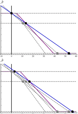
Figure 1 illustrates what happens once we introduce the leverage constraint. In the illustration, absent short sales the leverage constraint is satisfied. However, a sufficiently large position by short sellers can force the financial institution to liquidate some of its long-term asset holdings. These forced sales reduce the financial institution’s equity value equity because the long-term asset has to be sold at a discount to fundamental value (when sold at t= 1 it yields δR rather than R). Hence, the fundamental value of the financial institution’s equity has a kink at the point where the leverage constraint becomes binding and forces the financial institution to sell assets. To facilitate comparison to the benchmark case discussed above, the dashed line indicates the fundamental value of equity in the absence of the leverage constraint.
Recall the equilibrium condition,Pe=P. This condition implies that potential equilibria are intersections of the two lines in Figure 1, i.e., points where the price in the equity market at t= 1 rationally reflects the fundamental value of the equity of the financial institution at t= 2. Turn first to the top panel of Figure 1. We continue to assume that long-term investors choose the interceptP to be equal to fundamental value absent short sales, i.e.,P =XR−D0.13Because the two lines only intersect once, the only equilibrium remains the one without short selling—even though the short sellers can drive down the fundamental value of the financial institution by forcing it to liquidate some of its long-term investments, they invariably lose money in the process. This is the case whenever the liquidation value of the long-term asset, which is parameterized byδ, is sufficiently large. 13 As we show below, this assumption is not crucial in the sense that the equilibria are independent of the particular choice of P and λ. We focus on the case P =XR−D0 because it allows us to focus exclusively on predatory short selling. The main difference to the caseP̸=XR−D0is that now also the beneficial role of short selling (as discussed above) emerges.
In this case, the value destruction on response to a violation of the leverage constrained is small, such that predatory short selling is not profitable. The unique equilibrium is the one whereP=XR−D0. WhenP=XR−D0 this implies that the equilibrium amount of short selling is S= 0. More generally, when P ̸=XR−D0, short selling can occur in equilibrium, but only in its beneficial role of ensuring that prices are equal to the fundamentalXR−D0.
The bottom panel of Figure 1, on the other hand, shows that when δ is sufficiently small, predatory short selling can emerge. In this case, in addition to the equilibrium without short selling, two further equilibria emerge. Both of these additional equilibria involve predatory short selling: Short sellers cause a decrease in the financial institution’s equity value at t= 1, which forces the financial institution to liquidate long-term asset holdings to an extent that allows short sellers to break even. As is usually the case, the middle equilibrium is unstable (such that a small perturbation would lead to migration to either of the two stable equilibria).
Equilibrium prices are independent of λ and P.One convenient feature of our model is that, as long as short sellers are not restricted in the number of shares they can short, the equilibrium prices and the equilibrium amount of the long-term asset that the financial institution needs to liquidate are independent of the particularP andλchosen by the long-term investors. Hence, while there are many equilibria involving different combinations ofP,λandS, these equilibria are isomorphic in terms of equilibrium prices and liquidation quantities. One implication of this feature of the model is that while setting the interceptP equal to fundamental value absent short selling allows us to focus exclusively on predatory short selling, equilibrium prices and the existence of predatory short selling equilibria do not depend on this assumption.
Lemma 3. When short sellers are unconstrained in the size of the short position they take, the equilibrium prices and the amount that has to be liquidated by the financial institution is independent ofλandP.
This independence result is illustrated in Figure 2 for the case in which the leverage constraint is satisfied absent short selling. The top panel shows that whenλis decreased from 0.75 (dashed line) to 0.6 (solid line), the equilibrium amount of short selling changes, but equilibrium prices remain the same. The bottom panel shows that when, in addition, also the intercept P is increased from 32 to 34, the equilibrium prices again remain un-changed. In this case, the equilibrium in which P=RX−D0 exhibits beneficial short selling, while the other two equilibria exhibit predatory short selling.
Lemma 3 is convenient since it allows us to classify equilibria by looking only at equi-librium prices and the amount of the long-term asset that has to be liquidated by the financial institution.
Overview of Equilibria.We are now in a position to summarize the equilibria in the equity market att= 1. In the proposition, we focus on the case where the long-term asset is relatively illiquid, δ < γ. This is the case depicted in the right panel of Figure 1. The (less interesting) caseδ≥γis discussed in the appendix.
Proposition 1. In the presence of the leverage constraint (1), whenδ < γwe distinguish three regions.
-10 0 10 20 30 40 50 60 S 5 10 15 20 25 30 35 P, P P P -10 0 10 20 30 40 50 60 S 5 10 15 20 25 30 35 P, P P P
Fig. 1. Introducing the leverage constraint.When the leverage constraint is
introduced (in this figure,γ= 0.7), a sufficiently large short position can force the financial institution to liquidate some of its long-term asset holdings. In the top panel, the loss to the financial institution from liquidating the long asset is not large enough to make a predatory short position profitable (δ= 0.75). The only equilibrium is the one in which no predatory short selling occurs. In the bottom panel, on the other hand, we see that when the losses from liquidating the long-term asset are large enough, two predatory short selling equilibria emerge in addition to the equilibrium without predatory short selling (δ= 0.6). The middle equilibrium is unstable. The remaining parameters in this figure are:X= 10, R= 10, D= 68, λ= 0.75
1. Safety region:When the financial institution is sufficiently well capitalized,R >
D0
δX, there is a unique equilibrium in which the financial institution does not have
to liquidate any of its long-term holdings. No predatory short selling can occur,
∆X(S) = 0, andP=XR−D0.
2. Vulnerability region: When D0
γX ≤R≤ D0
δX, there are two stable equilibria and
one unstable equilibrium.
a. In one stable equilibrium, the financial institution does not liquidate any of its long-term holdings,∆X(S) = 0, andP =XR−D0.
-10 0 10 20 30 40 50 60 S 5 10 15 20 25 30 35 P, P -10 0 10 20 30 40 50 60 S 5 10 15 20 25 30 35 P, P
Fig. 2. Equilibrium prices are independent of P and λ. The top panel
shows that when λ is decreased from 0.75 (dashed line) to 0.6 (solid line), the equilibrium amount of short selling changes, but equilibrium prices remain the same. The bottom panel shows that when in addition also the intercept P is in-creased from 32 to 34, the equilibrium prices again remain unchanged. In this case, the equilibrium in whichP =RX−D0 exhibits beneficial short selling, while the other two equilibria exhibit predatory short selling. The remaining parameters are R= 10, X= 10, δ= 0.6, γ= 0.7, D= 68.
b. In the other stable equilibrium, the financial institution is forced to liquidate its entire holdings of the long-term asset, i.e.,∆X(S) =X andP= 0.
c. In the unstable equilibrium, the financial institution has to liquidate part of its equity holdings,∆X(S) =Xγ− D0 XR γ−δ andP = 1−γ γ−δ(D0−δXR)
3. Doomed region: WhenR < D0
γX, there is a unique stable equilibrium and an
un-stable equilibrium.
a. In the stable equilibrium, short sellers are active and the financial institution liquidates its entire holdings of the long-term asset,∆X(S) =X andP= 0.
b. In the region D0
γX > R > D0
δX(1+γ) an unstable equilibrium exists, in which
of the long-term asset holdings, ∆X(0) =X D0 XR−γ δ−γ(1−δ) and P=XR−D0− 1−δ δ−γ(1−δ)[D0−γXR].
Figure 3 illustrates the equilibria as a function of XR, the fundamental value of the financial institution’s long-term asset holdings. As Proposition 1 points out, there are three regions of interest. First, whenRis sufficiently high, short sellers cannot profitably force the financial institution to liquidate long-term asset holdings. In this region, the financially institution is sufficiently well-capitalized, such that the only equilibrium is the one in which the financial institution holds its long-term investments until maturity. We refer to this region as the safety region. In the safety region, short sellers solely fulfill the beneficial function of correcting the equity value of the financial institution when the long-term investors offer an intercept higher than the fundamental value of equity. One important implication from this region is that, when financial institutions are healthy one should not be concerned about predatory behavior by short sellers. Hence, our framework does not lend support to unconditional short selling bans.
However, whenRdrops sufficiently, there is a second region with multiple equilibria. In this region, the leverage constraint is satisfied if short sellers do not take predatory short positions. Hence, there still is an equilibrium without short selling and without liquida-tion by the financial instituliquida-tion. However, there are now also two equilibria in which short sellers take predatory short positions and force the financial institution to liquidate some or all of its long-term asset holdings. In this region, the financial institution is vulnerable to predatory short selling, even though absent short selling the leverage constraint is not binding. We thus refer to this region of multiple equilibria as thevulnerability region. This vulnerability region emerges only whenδ < γ, i.e., when the long-term asset held by the financial institution is sufficiently illiquid. This highlights the importance of liquidity mis-match (illiquid long-term assets financed with short-term credit) in facilitating predatory short selling.
Finally, there is a third region with two equilibria, on stable and one unstable. In the stable equilibrium, short sellers are active and force the financial institution to liquidate its entire asset holdings, such that the equity value of the financial institution is given by P = 0. In the unstable equilibrium, short sellers are not active and the financial institution liquidates part of its long-term asset holdings. Because in this region the unique stable equilibrium involves a complete liquidation of the financial institution, we refer to this region as thedoomed region.
The effect of banning short selling.We are now in a position to compare outcomes under a regime in which short selling is allowed and a regime in which short selling is prohibited. When short selling is restricted, the financial institution only needs to liqui-date at liqui-datet= 1 when the leverage constraint is violatedabsent predatory short sellers. Proposition 2 compares the two regimes, focusing on stable equilibria.
Proposition 2. Consider again the case δ < γ. The effect of banning short selling on equilibrium prices and the quantity of the long-term investment liquidated by the financial institution depends on the equilibrium region:
1. Safety region:When the financial institution is sufficiently well capitalized (R >
D0
δX), equilibrium prices and the amount the financial institution needs to liquidate
8 9 10 11 12 13 14
XR
20 40 60 80 100P
Doomed Region Vulnerability Region Safety Region short sellingHstableLshort sellingHunstableL no short sellingHunstableL no short sellingHstableL
Fig. 3. Overview of Equilibria. This plot shows the equilibrium equity value
of the financial institution as a function of R. For high values of R, there is a unique equilibrium without predatory short selling (safety region). Once Rdrops sufficiently low, there is a region with multiple equilibria (when γ > δ). In this
vulnerability region predatory short selling can emerge. The middle equilibrium is unstable. WhenRis so low that the leverage constraint binds in the absence of short selling, there is a stable equilibrium with predatory short selling and an unstable equilibrium without predatory short selling (the doomed region). The parameter values in this graph areX= 10, δ= 0.6, γ= 0.7, D= 68.
2. Vulnerability region:In the vulnerability region (D0
γX ≤R≤ D0
δX), when short
sell-ing is restricted no liquidation takes place and the unique equilibrium is given by
P =XR−D0 and ∆X= 0. When short sellers are present, on the other hand,
there is a second stable equilibrium, in which predatory short sellers force the fi-nancial institution to liquidate its entire long-term asset holdings: ∆X=X and
P = 0.
3. Doomed region: In the doomed region (R < D0
γX), when short selling is
re-stricted the financial institution liquidates part of its long-term asset holdings as long as R > D0 δX(1+γ). In this region, ∆X(0) =X D0 XR−γ δ−γ(1−δ) and P=XR−D0− 1−δ
δ−γ(1−δ)[D0−γXR]. When R≤ δXD(1+0γ), the financial institution liquidates its
entire long-term asset holdings even when short selling is restricted, and P = 0. When short sellers are present, in the doomed region the financial institution al-ways liquidates its entire holdings andP = 0.
Figure 4 illustrates the main differences between a regime with short selling (solid line) and a regime in which short selling is restricted (dashed line). First, note that when short
8 9 10 11 12 13 14
XR
20 40 60 80 100P
Doomed Region Vulnerability Region
Safety Region
Fig. 4. The effect of banning short selling. This figure compares equilibria
with and without short selling, focusing on stable equilibria. When short selling is allowed (solid line), there are multiple equilibria once the financial institution enters thevulnerability region. In one of the two stable equilibria, predatory short sellers force the financial institution to liquidate its entire long-term asset holdings. In thedoomed region, in the unique stable equilibrium short sellers always force the financial institution to unwind its entire asset holdings. When short selling is not allowed (dashed line), the financial institution does not have to liquidate in the vulnerability region andP =XR−D0. Moreover, in the doomed region, the financial institution only has to liquidate part of its long-term asset holdings when short selling is restricted (except whenRis so low that the financial institution has to liquidate everything even in the absence of short selling). The parameter values in this example areX = 10, δ= 0.6, γ= 0.7, D= 68.
sales are restricted, there is no vulnerability region—the financial institution only has to liquidate some of its long-term asset holdings if the leverage constraint is violated in the absence of temporary price movements caused by short sellers. When short selling is allowed, on the other hand, the vulnerability region emerges and there is a second equilibrium in which short sellers prey on the financial institution, forcing it to unwind its entire long-term asset holdings. Hence, in this region predatory short sellers can force a collapse of the financial institution, even though the financial institution would be sound in the absence of short selling.
Second, when the leverage constraint is violated even in the absence of short selling, the amount the financial institution has to liquidate is (weakly) smaller when short selling is restricted. This is the case because in the doomed region in the unique stable equilibrium short sellers force the financial institution to liquidate its entire portfolio. When no short sellers are present, on the other hand, the financial institution can in general satisfy the leverage constraint by selling only part of its long-term asset holdings, except when R
drops so low that the financial institution enters a “death spiral” (i.e, it has to liquidate all long-term asset holdings even when no short sellers are present). In the figure, this happens at the point where the dashed line meets the x-axis.
Of course, one caveat of the analysis above is that we have focused exclusively on the case in which, absent short selling, the equity of the financial institution is priced correctly. This allowed us to focus exclusively on characterizing the conditions under whichpredatory
short selling can occur. More generally, the potential welfare costs of predatory short
selling have to be weighed against the beneficial effects of regular short selling through the elimination of overvaluation and improvements in market quality and liquidity. As discussed above, in the safety region predatory short selling cannot occur and the only effect of short sellers is the elimination of mispricing. Clearly, in this region, a short-sale ban is not desirable. In the vulnerability region, on the other hand, the costs of potential predatory short selling have to be weighed against the potential benefits from regular short selling. The desirability of a potential short selling ban then depends on the relative size of these two effects. While formally our model does not deliver predictions on how large these two effects may be in practice, it does provide some informal guidance. For example, if one believes that a financial institution is only temporarily in the vulnerability region, a short selling ban may prevent the collapse of the financial institution, while the costs of temporary overvaluation of the financial institution’s equity might be moderate. Similarly, in the doomed region one would have to weigh the benefits of controlled deleveraging that is possible in the absence of short sellers against the potential costs of overvaluation in this region.
3.3 REGULAR SELLING VERSUS SHORT SELLING
Up to now our analysis has focused exclusively on short selling. In this section, we contrast our results to those that would obtain if we replaced short sellers with regular sellers (i.e., investors who have an initial endowment of shares in the financial institution). This will sharpen the distinction between regular selling and short selling and highlight the important role important role of coordination.
The distinction between short selling and regular selling is particularly relevant in the vulnerability region where, as shown above, multiple equilibria Pareto-ranked equilibria are possible: In the Pareto-dominant equilibrium, the financial institution does not have to sell any of its long-term asset holdings and survives. In contrast, in the dominated equilibrium, the financial institution is forced to liquidate all long-term asset holdings and fails. The discussion in this section revolves around the following questions: Can the dominated equilibrium also emerge in a setting with regular sellers as opposed to short sellers? If yes, is there reason to believe that it is more likely to emerge as a result of short selling as opposed to regular selling?
Recall that in the competitive setup developed above, when all trades are executed at the final market clearing price, short sellers are indifferent between the two equilibria that are possible in the vulnerability region—they make zero profits in either. More generally, if short sellers can walk down the demand curve when establishing their short position (i.e., when not all trades are executed at the final price) they strictly prefer the equilibrium in which they collectively prey on the financial institution. This contrasts with situation that would arise if short sellers were regular sellers: While a setup with regular sellers instead of short sellers would lead to the same two equilibria in the vulnerability region, regular
sellers strictly prefer the equilibrium in which they hold on to their shares and do not sell. Hence, with regular sellers, the dominated equilibrium can only emerge as a result of coordination failure—existing shareholders sell because they expect everyone else to sell, comparable to the dominated equilibrium in Diamond and Dybvig (1983). While this, of course, does not rule out the dominated equilibrium, it is a reasonable proposition that the dominated equilibrium is less likely to emerge through a pure coordination failure of regular sellers than through a (weakly) profitable attack by predatory short sellers.
In addition, as soon as we depart from the competitive benchmark and allow for some amount of coordination among short sellers or shareholders, the equilibrium regions dif-fer depending on whether sellers are regular sellers or short sellers. Specifically, some amount of coordination among short sellers increases the doomed region where the unique equilibrium involves a complete liquidation of the financial institution. In contrast, some amount of coordination among regular sellers increases the safety region where the unique equilibrium involves no liquidation.
Formally, we model the degree of coordination by assuming that there is a large trader or, equivalently, a mass of small traders who can coordinate their actions. The large trader (or coordinated traders) internalize that their trading decision moves the share price. The remaining traders form a competitive fringe and take prices as given. In the short selling case, we assume that the large short seller can take a maximum short position ofSMAX. In the case of regular sellers, we assume that the large shareholder ownsSMAX shares in the financial institution, while the competitive fringe owns SMAX
C shares. We
also assume that if both the large shareholder and the competitive fringe sell their shares, the share price drops to zero and the financial institution has to liquidate all of its long-term asset holdings. Formally, this assumption requires that in the regular selling case SMAX+SMAX
C =Se, whereSeis defined byPe=P−λSe= 0. Note that in both the regular
and the short selling caseSMAXproxies for the amount of coordination that is possible. For simplicity and to reflect the role of large traders (such as George Soros) as first movers, we assume that the large trader moves first and that the competitive fringe moves after the large trader’s order has been executed. However, as we describe in more detail below, the findings in Proposition 3 do not depend on the specific assumptions on move and execution order. For example, we could alternatively assume that the large trader and the competitive fringe submit their orders and are executed simultaneously, or that the execution order is random and traders submit limit orders. Both of these alternative setups would leave the equilibrium regions described in Proposition 3 unchanged (see footnotes 16 and 17 for more details).
Consider first the case of short sellers. The large short seller moves first and chooses S∈[0, SMAX]. The large short seller’s trade is then executed atP(S) =P−λS. Then, the competitive fringe moves and choosesSC. The orders of the competitive fringe are executed
atP(S+SC) =P−λ(S+SC). Whenever the maximum short position of the large short
seller, SMAX, is sufficiently large to make the short sale profitable irrespective of the actions of other short sellers, the unique equilibrium involves predatory short selling. This is the case wheneverSMAX> S∗, whereS∗ denotes the short position required to make a
short sale profitable (for a formal definition ofS∗, see equation (A7) in the appendix). This condition holds when the financial institution is sufficiently close to its leverage constraint. Hence, the presence of a large short seller expands the doomed region in which the unique equilibrium involves complete liquidation of the financial institution.
In contrast, in the case of regular sellers the presence of the large trader expands the safety region in which the unique equilibrium involves no liquidation by the financial
institution: This is the case when the blockholder’s decision not to sell his shares can ensure that no coordination failure occurs, which is the case whenSMAX>Se−S∗: Given that the large shareholder does not sell, the competitive fringe cannot profitably coordinate to sell because Pe(SMAX
C )< P(SMAXC ). The unique best response is thusSC= 0 and no
liquidation is the unique equilibrium.14 Solving for SMAX> S∗ and SMAX>Se−S∗ in
terms of the parameters of the model yields the following proposition.
Proposition 3. Assume that there is a large trader or, equivalently, a mass of small
traders that can coordinate there actions up to a maximum ofSMAX shares.
1. Short selling: If traders who coordinate up to SMAX are short sellers,
the doomed region (with a unique short selling equilibrium) expands to R∈
[ 0,min [ D0 γX + γ−δ (1−δ)γXλS MAX,D0 δX ]) .
2. Regular selling: If traders who coordinate up to SMAX are regular sellers,
the safety region (with a unique no-liquidation equilibrium) expands to R∈
( max [ D0 δX − γ−δ (1−γ)δXλS MAX,D0 γX ] ,∞ ) .
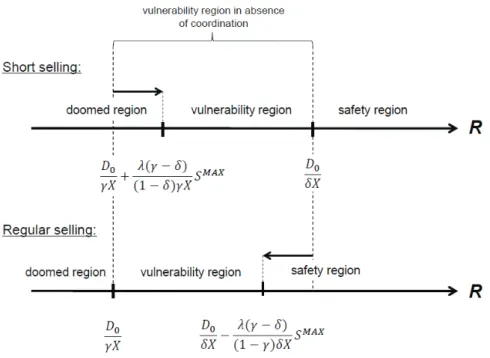
The equilibrium regions in the presence of a large trader are illustrated in Figure 5. The top panel illustrates the expansion of the doomed region in the presence of a large short seller. The bottom panel illustrates the expansion of the safety region in the presence of a large shareholder in the regular selling case.
Proposition 3 shows that once a certain amount of coordination is possible, there is a sharp difference between short selling and regular selling: While in both cases coordination shrinks the parameter vulnerability region (the region with multiple equilibria), in the short selling case this happens via an expansion of the doomed region (in which predatory short selling is the unique equilibrium), whereas in the case of regular sellers this happens through an expansion of the safety region (where no liquidation is the unique equilibrium). In the extreme, the vulnerability region vanishes completely. In the short selling case, the financial institution is then liquidated as soon as short sellers have the ability to force the financial institution to violate its leverage constraint (i.e., when R < D0
δX). In the case of
14 The role of the large short seller or blockholder discussed here is similar to the role of large players in the literature on currency crises. See, in particular, Corsetti, Pesenti, and Roubini (2002) and Corsetti, Dasgupta, Morris, and Shin (2004) for a setting in which traders face a binary decision on whether or not to attack a currency.
Fig. 5. Equilibrium regions under short selling and regular selling.The figure compares equilibrium regions under short selling and regular selling in the presence of a large trader (or a mass of small traders who can coordinate their actions) of sizeSMAX. The parameter region for which the unique equilibrium in-volves liquidation of the financial institution is larger under short selling than under regular selling. Conversely, the parameter region for which the unique equilibrium involves no liquidation by the financial institution is larger under regular selling than under short selling.
regular sellers, on the other hand, no liquidation occurs unless the financial institution violates its leverage constraint in the absence of short sellers (i.e., whenR < D0
γX).
15 16 17
15 One interesting implication of Proposition 3 is that the region in which the unique equilibrium involves predatory short selling depend on the slope of the demand curve λ, which we have taken as given here. This is the case when the position limit for the short seller are in terms of the maximum number of shares that can be shorted, SMAX. Alternatively, if position limits are defined as “price impact” limits (which would be of the formSMAX/λ), the region in which predatory short selling is the unique equilibrium is independent of the slope of the demand curve λ, thereby recovering the irrelevance property of Lemma 3.
16 If instead of sequential orders and execution we were to assume that orders are sub-mitted and executed simultaneously, the resulting equilibrium regions would be identical to those in Proposition 3. The main difference is that, in the simultaneous-move game, it is thethreat of the large short seller that eliminates the no-liquidation equilibrium. As
3.4 SUPPORT BUYING BY A LARGE TRADER
Next, we discuss the effect of adding investors who can step in to buy shares (recall that up to now the long-term investors that form the residual demand curve were assumed to be completely passive and thus never acted as active support buyers). To do this, consider the case in which both a large short seller (or a mass of short sellers who can coordinate) and a large support buyer (or a mass of traders who can coordinate to purchase stock in the financial institution) are present. We assume that the support buyer (this could, for example, be a blockholder or another large trader with a vested interest in the financial institution) can buy up to BMAX additional shares to support the financial institution. For simplicity, we set the support buyer’s initial endowment in shares of the financial institution to zero. As before, the large short seller can short a maximum ofSMAXshares. As in the previous subsection, we assume that the large traders (the short seller and the support buyer) trade first, followed by the competitive fringe.
In this case, the region in which predatory short selling is the unique equilibrium de-pends on the relative strengthof the support buyer vis-`a-vis the short seller. Specifically, starting from a conjectured no-liquidation equilibrium, the short seller’s maximum posi-tionSMAXmust now be sufficiently large to make deviation profitable even if the support buyer purchases the maximum amount of shares BMAX. If this is the case, the unique equilibrium involves predatory short selling. Similar to Proposition 3, we can then char-acterize the regions in which the unique equilibrium involves predatory short selling as follows:
Proposition 4. Assume that there is a large short seller or, equivalently, a mass of
small traders that can coordinate there actions up to a maximum ofSMAXshares. Assume
also that there is a large support buyer (or a mass of small support buyers coordinate)
who can purchase BMAX additional shares to support the share price of the financial
in-stitution. Then the doomed region (with a unique short selling equilibrium) is given by
R∈ [ 0,D0 γX + γ−δ (1−δ)γXλ [ SMAX−BMAX]+).
before, when SMAX> S∗, the large short seller has a strictly profitable deviation from a
conjectured no-liquidation strategy profile. However, the large short seller cannot be part of a zero-profit short selling equilibrium with S+SC=Se, because from any such
equi-librium he would have an incentive to slightly reduce the size of his short position and make positive (instead of zero) profits. Hence, whenSMAX> S∗the unique equilibrium is
a predatory short selling equilibrium in which the competitive fringe takes a short position ofSC=Sein response to thethreat of a short potions by the large short seller.
17 Also a setup with random execution order in which traders can submit limit orders leads to the same equilibrium regions. Because there is a one-to-one mapping between the execution price and the order of execution, limit orders allow traders to effectively condition their sell orders on when they are executed. If the large trader is executed first, the analysis is identical to the one discussed in the text (the analysis in the text is a limiting case of the more general limit order setup: the probability that the large trader is executed first is one). In the case where the large trader is executed after the competitive fringe, the equilibrium regions remain the same but in the coordination failure equilibrium the large shareholder may sell slightly less if he anticipates that his order will be executed after the competitive fringe (and thereby at a lower price). See the appendix for more details.