Some Models for Count Time Series

Clemson University

TigerPrints

All Dissertations

Dissertations

8-2018

Some Models for Count Time Series

Yisu Jia

Clemson University, [email protected]

Follow this and additional works at:

https://tigerprints.clemson.edu/all_dissertations

This Dissertation is brought to you for free and open access by the Dissertations at TigerPrints. It has been accepted for inclusion in All Dissertations by

an authorized administrator of TigerPrints. For more information, please [email protected].

Recommended Citation

Jia, Yisu, "Some Models for Count Time Series" (2018).All Dissertations. 2213.

Some Models for Count Time Series

A Dissertation Presented to the Graduate School of

Clemson University

In Partial Fulfillment of the Requirements for the Degree

Doctor of Philosophy Statistics by Yisu Jia August 2018 Accepted by:

Dr. Robert Lund, Committee Chair Dr. Peter Kiessler

Dr. Xin Liu Dr. Brian Fralix

Abstract

There has been growing interest in modeling stationary series that have discrete marginal distributions. Count series arise when describing storm numbers, accidents, wins by a sports team, disease cases, etc.

The first count time series model introduced in this paper is the superpositioning methods. It have proven useful in devising stationary count time series having Poisson and binomial marginal distributions. Here, properties of this model class are established and the basic idea is developed. Specifically, we show how to construct stationary series with binomial, Poisson, and negative binomial marginal distributions; other marginal distributions are possible.

A second model class for stationary count time series – the latent Gaussian count time series model – is also proposed. The model uses a latent Gaussian sequence and a distributional transfor-mation to build stationary series with the desired marginal distribution. This model has proven to be quite flexible. It can have virtually any marginal distribution, including generalized Poisson and Conway-Maxwell. It is shown that the model class produces the most flexible pairwise correlation structures possible, including negatively dependent series. Model parameters are estimated via two methods: 1) a Gaussian likelihood approach (GL), and 2) a particle filtering approach (PF).

Dedication

I dedicate this work to my loving parents – for their unconditional love and support. My family is the foundation for who I am.

Acknowledgments

First of all, I would like to thank my advisor Dr. Robert Lund. This work would not be completed without his guidance and support.

Secondly, I would like to thank my colleagues on the ”Latent Gaussian Count Time Series Modeling” project: Dr. Vladas Pipiras, Dr. James Livsey, and Dr. Stefanos Kechagias. Their mathematical insights inspired me a lot in my research.

I would also like to thank Dr. Peter Kiessler, Dr. Xin Liu, and Dr. Brian Fralix for their insightful advice.

Finally, I would like to thank the Department of Mathematical Sciences for supporting me financially during my Ph.D studies.

Table of Contents

List of Figures vii

1 Introduction 1

1.1 Time Series Overview . . . 1

1.2 Count Time Series . . . 3

1.3 Research Motivations . . . 9

2 Superpositioned Stationary Count Time Series 10 2.1 Stationary Zero-One Series . . . 11

2.2 Superpositioning . . . 13

2.3 Classical Count Marginal Distributions . . . 14

2.4 Other Marginal Distributions . . . 20

2.5 Comments . . . 23

3 Latent Gaussian Count Time Series Modeling 24 3.1 Theory . . . 25

3.2 Particle filtering and the HMM connection . . . 35

3.3 Inference . . . 42

3.4 A Simulation Study . . . 46

3.5 An Application . . . 50

A Appendices 54 A.1 Proof of Theorem 2.2.1 in Chapter 2 . . . 54

A.2 Proofs of results in Chapter 3 . . . 58

List of Tables

3.1 Optimized log likelihood with the AIC/BIC for different latent Gaussian structures. 51 3.2 Estimates and standard errors of the full model with{Zt} being AR(1). . . 52

List of Figures

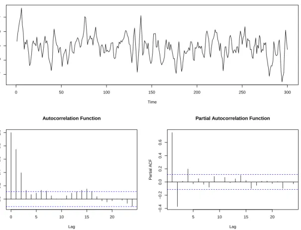
1.1 Realization of 300 observations of a ARMA(1,2) withφ1= 0.5, θ1= 0.5, θ2= 0.3. . . 4

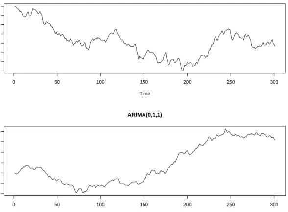
1.2 Top: realization of 300 observations of an ARIMA(1,1,0) series with φ1= 0.3.

Bot-tom: realization of 300 observations of an ARIMA(0,1,1) series withθ1= 0.5. . . 5

1.3 Annual number of Atlantic tropical cyclones from 1850 to 2011. . . 6 2.1 Two hundred points of a stationary count time series with Bin(5,0.5) marginal

distri-bution. Sample autocorrelations and partial autocorrelations are shown with point-wise 95% confidence bands for white noise. . . 15 2.2 A realization of a stationary count time series with Poisson marginal distributions

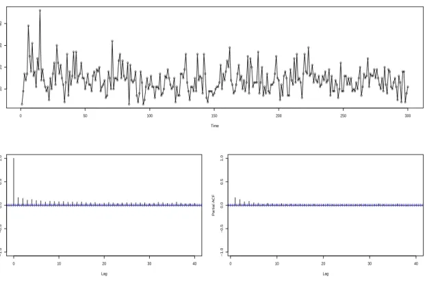
with mean 5. Sample autocorrelations and partial autocorrelations are shown with pointwise 95% critical intervals for white noise. . . 17 2.3 A realization of a long memory stationary count time series withN B(10,0.5) marginal

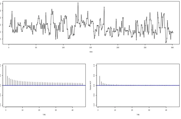
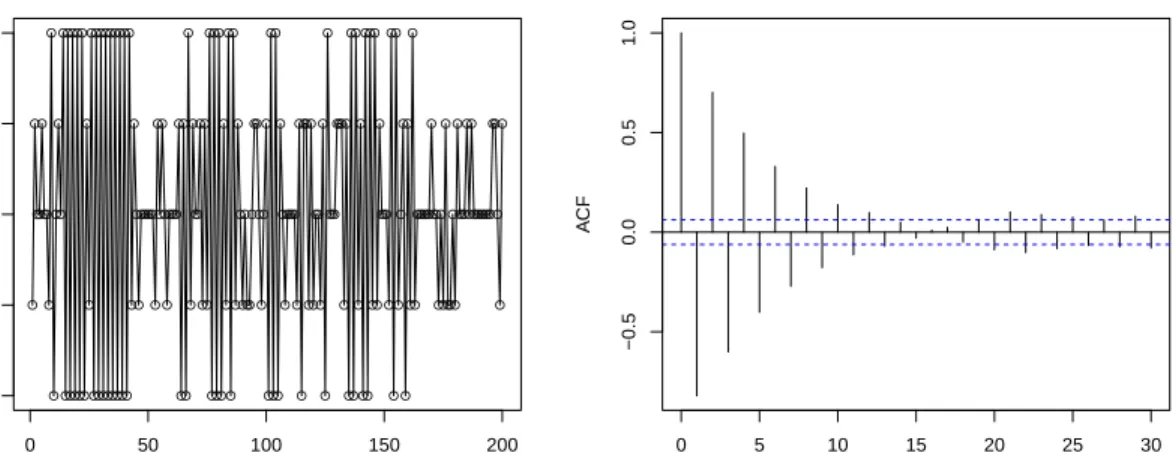
distributions. Sample autocorrelations and partial autocorrelations are shown with pointwise 95% confidence bounds for white noise. . . 18 2.4 A realization of a stationary count time series withN B(10,0.5) marginal

distribu-tions. Sample autocorrelations and partial correlations are shown with pointwise 95% confidence bounds for white noise. . . 20 2.5 A realization of a stationary count time series with discrete uniform marginal

support-ed on {1,2,3,4,5}. Sample autocorrelations and partial autocorrelations are shown with pointwise 95% confidence bounds for white noise. . . 22 3.1 The link coefficients hk on a log-vertical scale for the Poisson (left) and negative

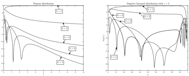
binomial (right) distributions. . . 33 3.2 The link functionh(u) for the Poisson distribution withλ= 0.1, 1, and 10 (left) and

the negative binomial distribution withr= 3 andp= 0.1, 0.5, and 0.95 (right). . . . 34 3.3 Estimates from simulated Poisson AR(1) series. In the left plots, the true value of

parameters areλ= 2 and φ= 0.75. In the right plots, the true value of parameters areλ= 2 andφ=−0.75. All true parameter values are plotted as a horizontal red dashed line. Sample sizes of 100, 200, and 400 are indicated on the horizontal axis and estimation method are given in the legend. . . 47 3.4 Estimates from simulated Mixed Poisson AR(1) series. In the left plots, the true

parameter values areλ1 = 2, λ2 = 5, φ= 0.75 andp= 1/4. In the right plots, the

true parameter values areλ1 = 2,λ2 = 10, φ= 0.75 andp= 1/4. True values are

shown as a red horizontal dashed line. Sample size of 100, 200 and 400 are given on the horizontal axis and estimation method are indicated in the legend. . . 48

3.5 Estimates from simulated Negative Binomial MA(1) series. In the left plots, the true value are r= 3, p= 0.2 andθ = 0.75. In the right plots, the true value arer= 3, p= 0.2 andθ=−0.75. True values are shown as red horizontal dashed line. Sample sizes of 100, 200 and 400 are given on the horizontal axis and estimation method are indicated in the legend. . . 49 3.6 The number of no-hitters pitched by season from 1893 to 2017 and its sample

au-tocorrelation and partial auau-tocorrelations. Pointwise 95% confidence intervals are displayed. . . 50 3.7 The upper left is the plot of the estimated residuals against time. The upper right

is the QQ plot the estimated residuals. The two plots on the bottom are the sample ACF and sample PACF plot of the estimated residuals. . . 53

Chapter 1

Introduction

1.1

Time Series Overview

A time series is a sequence of random variables collected over time. Most often, the mea-surements are made at regular time intervals. Time Series Analysis is used in many applications, including: economic forecasting, sales forecasting, stock market analysis, sports analysis, and many more.

The basic objectives of time series modeling are to fit a model that describes the structure of the time series and provides real-world interpretations. Uses for a fitted model are:

• To describe the important features of the time series, such as trend, seasonality, and change-points.

• To explain how the past affects the future, thus to permitting forecasting of future values of the series.

One difference of time series analysis from regression analysis is that the data are not necessarily independent. LetX1, X2,· · ·, Xn be a time series of lengthn, denoted as{Xt}nt=1. The

mean structure of{Xt}nt=1 isµt :=E[Xt]. The covariance structure of{Xt}nt=1 is described by its

autocovariance function (ACVF). The laghACVF at timetis defined as

A time series {Xt} is said to be weakly stationary if it satisfies: 1) the mean E(Xt) is

the same for all t, 2) the covariance between Xt and Xt+h is the same for all t and every h ∈

{0,1,2,· · · }. Similarly, a time series{Xt}is said to be strictly stationary if (X1, X2,· · · , Xn)0 and

(X1+h, X2+h,· · ·, Xn+h)0 have the same joint distribution for all integerh≥0 andn >0. Clearly,

strictly stationary implies weakly stationary.

For a (weakly) stationary series {Xt}, the lag hACVF does not depend on t for allh. In

this setting,

γX(t, t+h) =γX(0, h).

For notational convenience, one can use a single argument in all ACVFs: γX(h) :=γX(0, h).

In some cases, it is easier to look at correlations instead of covariances. The autocorrelation function (ACF) of a stationary time series{Xt} is defined as

ρ(h) := Corr(Xt, Xt+h) =

γ(h) γ(0).

Clearly, ACFs are between -1 and 1 by Cauchy-Schwarz inequality. In ACFs, the effect of dispersion in the series is removed. ACFs can be used to compare the level of dependency in different series.

For some series, it is worthwhile to pursue a partial autocorrelation function (PACF). In general, a partial correlation is a conditional correlation. For a time series, the partial autocorrelation between Xt and Xt+h, h ≥ 0, is defined as the conditional correlation between Xt and Xt+h,

conditional onXt+1, Xt+2,· · ·, Xt+h−1:

κ(h) := Corr(Xt, Xt+h|Xt+1,· · · , Xt+h−1),

where the conditional correlation is taken betweenXtandXt+hafter linear prediction of all variables

betweenXtandXt+h.

1.1.1

ARMA and ARIMA Models

In stationary time series analysis, the most commonly-used model class is the autoregressive moving average (ARMA) model class. The general ARMA model was described in the thesis of Peter Whittle ([36]) and was popularized in the 1970 book by Box and Jenkins ([4]). The ARMA model

class relates the current observation of a series to past observations and past prediction errors. An ARMA(p, q) model includes autoregressive terms up to order p and moving-average terms up to orderq. It obeys the recursion

Xt−φ1Xt−1−φ2Xt−2− · · · −φpXt−p=θ1Zt−1+θ2Zt−2+· · ·+θqZt−q,

where pandq are non-negative integers. The series{Zt} is white noises, that is often assumed to

be independent and identically distributed in timet. Whenp= 0, an ARMA(p, q) model is referred to as a moving-average model of orderq (MA(q)). Similarly, when q = 0, this model is called an autoregressive model of orderp(AR(p)). For the model to remain stationary, some constraints need to be met on the values of the parameters. For example, the AR(1) model is stationary with|φ1| 6= 1 and not stationary with |φ1| = 1. A realization of 300 observations of an ARMA(1,2) series with φ1= 0.5, θ1= 0.5, θ2= 0.3 is shown in Figure 1.1.

For non-stationary series, autoregressive integrated moving average (ARIMA) models can be used to describe patterns in the series. The elements in the model are specified in the form ARIMA(p, d, q), which include p autoregressive terms, q moving average terms, and d difference operations. More formally, a process{Xt}is said to be ARIMA(p, d, q) if

(1−B)dXt

is ARMA(p, q), where p, d, q are non-negative integers. Here, (1−B)d _{is thedth order difference}

operator. For example, (1−B)Xt=Xt−Xt−1,(1−B)2Xt= (1−B)(Xt−Xt−1) =Xt−2Xt−1+

Xt−2,· · ·. An ARIMA (1,1,1) model, for example, has one AR parameter and one MA parameter.

A first-order difference allows for a linear trend in the data. Realizations of ARIMA(1,1,0) and ARIMA(0,1,1) series of lengthn= 300 are shown in Figure 1.2.

1.2

Count Time Series

There has been significant recent interest in modeling stationary series that have dis-crete marginal distributions. Often, the disdis-creteness arises in the form of counts taking values

ARMA(1,2) Time 0 50 100 150 200 250 300 −4 −2 0 2 4 0 5 10 15 20 0.0 0.2 0.4 0.6 0.8 1.0 Lag A CF Autocorrelation Function 5 10 15 20 −0.4 −0.2 0.0 0.2 0.4 0.6 Lag P ar tial A CF

Partial Autocorrelation Function

Figure 1.1: Realization of 300 observations of a ARMA(1,2) withφ1= 0.5, θ1= 0.5, θ2= 0.3.

by a sports team, disease cases, etc. An example of a count time series is shown in Figure 1.3. It shows the annual number of Atlantic tropical cyclones from 1850 to 2011. The observation at each time is integer-valued, which clearly cannot be normally distributed.

The traditional ARMA/ARIMA model classes work well in describing series with Gaussian marginal distributions. However, no one definitive model class dominates the count series literature. In fact, the autocovariance function of many commonly used count models is deficient in some senses, as described below.

The theory of stationary Gaussian time series is well developed by now. However, there is no known result characterizing autocovariance functions of stationary count series. Elaborating,γX(·)

is a symmetric non-negative definite function on the integers, if and only if there exists a stationary Gaussian sequence{Xt}with Cov(Xt, Xt+h) =γX(h) for all integersh. Here, non-negative definite

ARIMA(1,1,0) Time 0 50 100 150 200 250 300 −35 −25 −15 −5 0 ARIMA(0,1,1) Time 0 50 100 150 200 250 300 −20 0 10 20 30 40

Figure 1.2: Top: realization of 300 observations of an ARIMA(1,1,0) series withφ1= 0.3. Bottom:

realization of 300 observations of an ARIMA(0,1,1) series withθ1= 0.5.

is defined as n X i=1 n X j=1 aiγX(ti−tj)aj ≥0

for every choice ofn∈ {1,2. . . ,} and real numbers a1, . . . , an. Unfortunately, no analogous result

exists for say, a stationary series with Poisson marginal distributions. In fact, restrictions on autoco-variance functions of count time series are often more stringent than just non-negative definiteness. For example, it may not be possible to have a stationary count series having a specific marginal distribution that is highly negatively correlated at some lag while the autocovariance function can take on any value between -1 and 1 in a Gaussian process.

Figure 1.3: Annual number of Atlantic tropical cyclones from 1850 to 2011.

1.2.1

DARMA Models

Initial attempts to model stationary count series used the discrete-valued autoregressive moving-average (DARMA) methods introduced in the 1970s by Jacobs and Lewis ([14, 15]). The model used mixing techniques to build series with preset marginal distributions. For example, a first order discrete autoregressive (DAR(1)) series {Xt} is built from independent and identically

distributed (IID) count variables {Yt}, say with marginal cumulative distributionF(·), and an IID

Bernoulli thinning sequence{Vt} with P(Vt = 1) := ρ∈[0,1]. The count series is initialized with

X0=Y0and then recursively updated via

Induction shows thatXt has distributionF(·) for every t∈ {1,2, . . .}.

While one can build any marginal distribution for a DAR(1) series (in addition to discrete structures), there are some undesirable properties of DARMA series. Foremost, DAR(1) sample paths can remain constant for long runs. Since_P(Xt=Xt−1)≥ρ, this issue becomes problematic

for larger ρ. DAR(1) models cannot produce negatively correlated series either. This is because the thinning probabilityρmust lie in [0,1]. In fact, one can show that the DAR(1) autocorrelation has form Corr(Xt, Xt+h) = ρh for all h≥ 0. While higher order autoregressions can be built by

introducing additional IID Bernoulli trial sequences, negative correlations cannot be achieved with any DAR formulation. An example where negatively correlated count series are encountered with hurricane counts is introduced by Livsey in 2018 ([19]). In short, the DARMA covariance structure cannot be expected to describe all stationary count series. For these reasons and more, DARMA models fell out of favor in the 1980s.

1.2.2

INARMA Models

Another count time series model, and one that remains popular today, is the integer ARMA (INARMA) model class. INARMA models were introduced by Steutel in 1979 ([29]) and stud-ied further in a series of papers in the 1980s ([1, 22, 23, 24]). For example, a first-order integer autoregressive (INAR(1)) model for{Xt} obeys the recursion

Xt=α◦Xt−1+t.

Here, ◦ denotes a thinning operator that acts on a count-valued random variate Y viaα◦Y :=

PY

i=1Bi, where{Bi} ∞

i=1 is a sequence of zero/one Bernoulli trials withP(Bi = 1) =α∈[0,1] and

{t}is a sequence of IID count-valued random variables with meanµ and finite varianceσ2.

Unlike DARMA series, INARMA sample paths do not tend to stay constant for long runs; however, like the DARMA class, INARMA models cannot have negative correlations. In fact, the INAR(1) model has Corr(Xt, Xt+h) = αh for any h ≥0. One can construct higher order integer

autoregressions and even add moving-average components as in [22, 23, 24]; however, one will not obtain a model with any negative correlations. Unlike DARMA series, it is not clear how to obtain any marginal distribution with INARMA methods — this, in fact, may be hard or impossible, depending on the marginal distribution desired.

1.2.3

Convolution-closed Infinitely Divisible Model Class

Another count series model type was proposed by Joe in 1996 ([16]). It produces stationary series whose marginal distribution lies in the so-called convolution-closed infinitely divisible class. Suppose that Fθ is a marginal distribution whose convolution, denoted by∗, satisfies Fθ1 ∗Fθ2 =

Fθ1+θ2. For the first order autoregressive case, the count series{Xt} obeys the recursion

Xt=At(Xt−1;α) +t,

where{t}are IID variables having the marginal distribution F(1−α)θ, α∈[0,1], andtis

indepen-dent ofXj forj < t. The operatorAt, which is IID in timet, is defined so that At(Y) is a random

variable whose marginal distribution is Fαθ (see [16] for details). These models capably describe

many marginal distributions — both discrete and continuous — and include gamma, beta, normal, binomial, Poisson, negative binomial, and generalized Poisson. However, the marginal distribution must come from the convolution-closed class. Unfortunately, again the correlations of these models cannot be negative.

1.2.4

RINAR Models

Recently, [17] produced negatively correlated count series models by rounding solutions to Gaussian autoregressive models. For example, a rounded autoregressive model of order pwith location parameterµand autoregressive parametersφ1, . . . , φp obeys

Xt= * µ+ p X j=1 φjYt−j + +t,

where hxi, for x ≥ 0, rounds x to its nearest integer (round down should this be non-unique),

{Yt} is a Gaussian autoregressive series, and {t} is count-valued IID noise. While such{Xt} can

have negative correlations, due to the rounding, it is difficult to construct a pre-specified marginal distribution in this model class.

1.3

Research Motivations

All historical count models devised to date have some nice features and individualized draw-backs. Bayesian approaches also exist for many count analyses, which usually do not demand a fixed marginal distribution. This dissertation focuses on building stationary count models with possibly negative and positive autocovariances while maintaining a fixed marginal distribution.

Another drawback of previous models is that none of them can generate count time series with long memory autocovariances. A stationary count series {Xt} is said to have long memory

ifP∞

h=0|cov(Xt, Xt+h)|=∞. Methods of constructing count series with long memory will also be

illustrated.

In what follows, Chapter 2 and 3 will introduce two methods for devising count time series that have desirable properties. Chapter 2 will build on the work of Cui and Lund ([7]), devising some count models where explicit autocovariance expressions are achieved. Chapter 3 then presents a very general copula-based technique. Here, explicit autocovariance expressions are not produced; however, a Hermite polynomial expansion provides series expressions that are very useful numeri-cally.

Chapter 2

Superpositioned Stationary Count

Time Series

This chapter introduces a different approach to model stationary count time series. Our count time series will be built from a stationary zero-one (binary) random sequence {Bt}. This

tactic was used in [3] and further developed in [7] and [21]. The idea can be viewed as the time series extension of the fact that any discrete-valued distribution can be constructed from fair coin flips.

For notation, let pB = E[Bt] ≡ P(Bt = 1) be the mean of {Bt} and denote its lag-h

autocovariance byγB(h) = Cov(Bt, Bt+h). Then

γB(h) =P(Bt= 1∩Bt+h= 1)−p2B=pB[P(Bt+h= 1|Bt= 1)−pB]. (2.1)

Two quantities that will be important later are theh-step-ahead transition probabilities to a unit point: p1,1:=P(Bt+h,i= 1|Bt,i= 1) andp0,1:=P(Bt+h,i= 1|Bt,i= 0). Obviously, the two

h-step-ahead transition probabilities to a zero point are p1,0 :=P(Bt+h,i = 0|Bt,i = 1) = 1−p1,1

2.1

Stationary Zero-One Series

2.1.1

Renewal zero-one point processes

We now discuss two models to efficiently construct {Bt}; other methods are also possible.

Our first model uses the renewal times in a stationary discrete-time renewal process as in [3, 7, 21]. A stationary renewal process employs an initial random “lifetime” L0 ∈ {0,1, . . .} (delay) and a

sequence of IID aperiodic lifetimes {Li}∞i=1 supported in {1,2, . . .} with µL := E[L1] < ∞. The

random walk {Sn}∞n=0 associated with the renewal process obeysSn =P n

i=0Li forn∈ {0,1, . . .}.

The zero-one process{Bt}is simply set to unity at all renewal times:

Bt=1[∪∞

n=0{Sn=t}].

To have {Bt} stationary, L0 needs to be specially selected as the so-called first-derived

distribution from the tails ofL1 [12]:

P(L0=k) = P

(L1> k)

µL

, k∈ {0,1, . . .}.

The Elementary Renewal Theorem givespB =µ−L1 and P(Bt+h= 1|Bt= 1) =uh, whereuh is the

probability of a renewal at timehin a so calledzero-delayed process (L0= 0). Equation (2.1) now

yields γB(h) = Cov(Bt, Bt+h) = 1 µL uh− 1 µL , (2.2)

Notice that γB(h) <0 if and only if uh < µ−L1, which happens for many renewal sequences. The

parameters in a renewal binary sequence are those that describe the lifetimeL1. In what follows,L

will denote a lifetime whose distribution is equivalent to any ofL1, L2, . . .. Point probabilities are

p1,1=uh andp0,1=pB(1−uh)/(1−pB).

2.1.2

Clipped Gaussian Sequences

A second construct for {Bt} uses a correlated latent Gaussian process {Zt} as in [19].

Specifically, let {Zt} be a correlated zero-mean unit-variance Gaussian random processes with

binary sequence withpB = 1−Φ(κ); here, Φ(·) denotes the cumulative distribution function of the

standard normal random variable. This construct is very similar to the clipping tactics introduced in [30].

The autocovariance function of {Bt}can be derived from bivariate normal probability

cal-culations. As an illustration, suppose that κ= 0 so that pB = 1/2. Then a classical multivariate

normal orthant probability calculation gives

E(BtBt+h) =P(Zt>0∩Zt+h>0) =

1 4 +

sin−1(ρZ(h))

2π ,

where [28] is used. SinceE[Bt]≡1/2,

γB(h) =

sin−1(ρZ(h))

2π , ρB(h) =

2 sin−1(ρZ(h))

π . (2.3)

In this case, laghautocovariances and autocorrelations are negative if and only ifρZ(h)<0. Hence,

this model can assume negative covariances. Notice thatρB(h) can take on any value in [−1,1].

When pB 6= 1/2, one will need to invert the standard normal cumulative distribution to

find the desired quantile of the standard normal distribution corresponding to pB. The covariance

function in this case is harder to derive explicitly as it involves integrating the bivariate normal density over an infinite rectangle that is not an orthant. For notation, defineG(x1, x2, ρ) :=P(Z1>

x1, Z2 > x2) for a bivariate normal random vector (Z1, Z2)0 with zero-mean, unit variance, and

correlationρ. A recent result on bivariate normal quadrant probabilities [19] gives

G(x1, x2, ρ) = 1−Φ(x1)−Φ(x2) + 1 4 ∞ X m=0 (2ρ)2m (2m)! 2x1x2F1(m+1₂;3₂;− x2 1 2 )F1(m+ 1 2; 3 2; −x2 2 2 ) Γ2₍1 2−m) +1 4 ∞ X m=0 (2ρ)2m+1 (2m+ 1)! F1(m+1₂;3₂; x2 1 2 )F1(m+ 1 2; 3 2; x2 2 2) Γ2₍1 2−m) ,

where F1(·;a, b) is the confluent hypergeometric function of the first kind with parameters a and

b: F1(x;a, b) = P∞_n=0(a)nx!/[n!(b)n], where (a)n is the rising factorial defined by (a)0 = 1 and

(a)n=a(a+ 1)(a+ 2)· · ·(a+n−1). In these expressions,x! = Γ(x+ 1) forx >0 and Γ(−x) for a

non-integerx >0 is defined via the recursion Γ(x+ 1) =xΓ(x). Turning to covariances,

E[BtBt+h] =G(κ, κ, ρZ(h)) = Z ∞ κ Z ∞ κ expx2−2ρZ(h)xy+y2 2[1−ρZ(h)2_] 2πp1−ρZ(h)2 dydx

andγB(h) =G(κ, κ, ρZ(h))−p2B. Transition probabilities can be verified as

p1,1= G(κ, κ, ρZ(h)) 1−Φ(κ) , p0,1= 1−Φ(κ)−G(κ, κ, ρZ(h)) Φ(κ) .

2.2

Superpositioning

We now move to superpositioned count series. Let{Bt,i}fori∈ {1,2, . . .}denote IID copies

of{Bt}. Our count series{Xt} is built by superimposing a random number of IID copies of{Bt}:

Xt= Mt X

i=1

Bt,i. (2.4)

Here, {Mt} is an IID count-valued random sequence that is independent of all{Bt,i}. See [2] for

more when{Mt}is a Poisson process.

Let E(Mt) =µM and var(Mt) = σM2 . It is obvious that {Xt} in (2.4) is a count-valued

strictly stationary random sequence with mean _E[Xt] ≡ pBµM. The following result establishes

additional properties of{Xt}.

Theorem 2.2.1. Let{Xt} be the strictly stationary count series in (2.4). Then

a) The probability generating function ofXthas formψX(u) :=E[uXt] =ψM(1−pB+pBu), where

ψM(u) :=E[uMt] is the probability generating function of Mt.

b) The dispersion of{Xt}isDX :=var(Xt)/E[Xt] =pBDM+ 1−pB, where DM :=σM2 /µM is the

dispersion ofMt. Xt is over/under dispersed if and only ifMt is over/under dispersed.

c) The lag h autocovariance of {Xt} Has the form γX(h) = κγB(h), where κ = E[min(M1, M2)]

when h6= 0, andγX(0) =γB(0)µM+p2Bσ2M.

d) The lag hbivariate probability distributions of{Xt} have form

P(Xt=xt, Xt+h=xt+h) = ∞ X mt=0 ∞ X mt+h=0 Hmt,mt+h(xt, xt+h)fM(mt)fM(mt+h),

where fM(k) =P(Mt=k)andHmt,mt+h(xt, xt+h)has the form identified in the Appendix.

e) In the renewal case, {Xt} has long memory if and only if E[L2] =∞. In the clipped Gaussian

case, {Xt} has long memory if and only if{Zt} has long memory.

This theorem is proven in appendix A.1. Attempts to derive higher order (beyond bivariate) joint process distributions have not produced tractable expressions to date. This is unfortunate as it precludes using the processes’ joint distribution to construct likelihood-based parameter estimators; nonetheless, the bivariate distribution above allows one to compute composite likelihood estimators [26, 25] and the covariance structure of the model permits pseudo-Gaussian likelihood parameter estimation.

2.3

Classical Count Marginal Distributions

This section constructs stationary time series with the classical count marginal distributions: binomial, Poisson and negative binomial.

2.3.1

Binomial Marginals

Count time series with binomial marginal distributions withM trials and success probability pB are easily obtained: just takeMtequal to the constant M. The binomial distribution is

under-dispersed withDX= 1−pB. This model was introduced by [3] and studied further in [7], [8], [33],

and [32]. By part c) of Theorem 1, when h6= 0, the lag hautocovariance and autocorrelation of

{Xt} are

γX(h) =M γB(h), ρX(h) =

γB(h)

pB(1−pB)

,

andγX(0) =M pB(1−pB),ρX(0) = 1. Then by (2.2), in the renewal case, the laghautocovariance

and autocorrelation of{Xt} are

γX(h) = M µL uh− 1 µL , ρX(h) = 1 µL uh−_µL1 pB(1−pB) .

From our derived expressions in the clipped Gaussian case, the lag hautocovariance and autocorrelation of{Xt} are, forh6= 0,

● ● ● ● ● ● ● ● ● ● ●● ● ●●● ● ● ●●● ●● ● ● ● ● ● ● ● ● ● ● ● ● ●● ● ● ● ● ● ● ● ●● ● ● ● ● ● ● ● ● ● ● ●● ● ● ● ● ● ● ● ● ●● ● ●● ● ● ● ●● ● ● ● ● ● ● ● ● ● ● ● ● ● ●● ● ● ● ●●●● ● ● ● ● ● ● ● ● ● ● ● ● ●● ●●● ● ● ● ●● ● ● ● ● ● ● ● ● ● ● ● ● ● ● ● ● ● ● ● ● ● ●● ● ● ● ● ● ● ● ● ● ● ● ● ● ● ● ● ● ● ● ●●● ● ●● ● ● ● ● ● ● ● ● ● ● ● ● ● ●●● ●● ● ● ● ● ● ● ● ● ● ● ● ● ●● 0 50 100 150 200 0 1 2 3 4 5 time count 0 5 10 15 20 25 30 35 −0.5 0.0 0.5 1.0 Lag A CF

Figure 2.1: Two hundred points of a stationary count time series with Bin(5,0.5) marginal distribu-tion. Sample autocorrelations and partial autocorrelations are shown with pointwise 95% confidence bands for white noise.

γX(h) =MG(κ, κ, ρZ(h))−p2B , ρX(h) = G(κ, κ, ρZ(h))−p2B pB(1−pB) .

Figure 2.1 shows a simulated realization of such a series. Here, the Bt,is were generated

from a renewal process with lifetimeLsupported on {1,2,3}, with P(L= 1) =P(L= 3) = 0.1 and

P(L = 2) = 0.8. Here, E[L] = 2 and pB = 1/2. From the sample autocorrelations plotted, it is

evident that negative correlations are obtained.

2.3.2

Poisson Marginals

To construct a count time series{Xt}with Poisson marginal distributions with meanλ >0,

let {Mt} be an IID Poisson sequence with mean λ/pB. It is easy to show thatXt in (2.4) has a

Poisson distribution with meanλ(see [7]). The Poisson distribution has unit dispersion. The lagh autocovariance of this process has form γX(h) =κγB(h), forh6= 0, whereκ=E[min(Mt, Mt+h)]

and Mt and Mt+h are independent Poisson random variables with mean λ/pB. This is derived in

[21] as κ= λ 1−e−2λ/pB_[I 0(2λ/pB) +I1(2λ/pB)] pB ,

whereIi(x) is the modified Bessel function Ii(x) = ∞ X n=0 (x/2)2n+i n!(n+i)!, i∈ {0,1}.

When h = 0, E[min(Mt, Mt+h)] = λ/pB. By Theorem 4.1, the lag h autocovariance of {Xt} is

γX(h) =κγB(h) whenh6= 0 andγX(0) =λ. In the renewal case, autocovariance and autocorrelation

functions are γX(h) = κ µL uh− 1 µL , ρX(h) = κ λµL uh− 1 µL .

Observe thatγX(h)<0 whenuh< µ−L1, which happens for many renewal lifetimesL. In the clipped

Gaussian case, the autocovariance and autocorrelation are

γX(h) =κ[G(κ, κ, ρZ(h))−p2B], ρX(h) =

κ

λ[G(κ, κ, ρZ(h))−p

2

B];

these are negative at laghwhenρZ(h)<0.

Figure 2.2 shows a simulated realization of a stationary count time series with Poisson marginal distributions with meanλ= 5. TheBt,is are generated from a clipped Gaussian process

– a zero-mean unit variance AR(1) series with lag one autocorrelation of 0.9.

2.3.3

Negative Binomial Marginals

Count series with negative binomial marginal distributions are often used to model overdis-persed count series [34, 31, 13]. The negative binomial distribution with parameters r∈ {1,2, . . .}

andp∈(0,1) (NB(r, p)) has the probability mass function

P(Xt=k) = _r+k −1 r−1 pr(1−p)k, k∈ {0,1,· · · }.

The dispersion of this distribution isDX = 1/(1−p)>1 and its probability generating function is

ψXt(u) =E[u Xt_{] = p} 1−(1−p)u r , |u|<(1−p)−1.

To construct a negative binomial count series {Xt} via the superposition in (2.4), apply

● ● ● ● ● ● ● ● ● ● ● ● ● ● ● ● ●● ●● ● ● ● ● ● ● ● ● ● ● ● ● ● ● ● ● ● ● ● ● ● ● ● ● ● ● ● ● ● ● ● ● ● ● ● ● ● ●● ● ● ● ● ● ● ● ● ● ● ●● ● ● ● ● ● ● ● ● ●●● ● ● ● ●●●●● ●●● ● ● ● ● ● ● ● ● ●● ● ● ● ● ● ● ● ● ● ● ●● ● ● ● ● ● ● ●● ● ● ● ● ● ● ● ● ● ● ● ● ● ● ● ● ●● ● ● ● ● ● ● ● ● ● ● ● ● ● ● ● ● ● ● ● ●● ● ● ● ● ● ● ● ● ● ● ●● ● ● ● ● ● ● ● ● ● ● ● ● ● ● ● ● ● ● ● ● ● ● ● ● ● ● 0 50 100 150 200 0 2 4 6 8 10 12 time count 0 5 10 15 20 25 30 −0.2 0.0 0.2 0.4 0.6 0.8 1.0 Lag A CF

Figure 2.2: A realization of a stationary count time series with Poisson marginal distributions with mean 5. Sample autocorrelations and partial autocorrelations are shown with pointwise 95% critical intervals for white noise.

ψM(u) = ppB 1−p+ppB 1− ppB 1−p+ppBu !r .

From this, it follows that the marginal distribution of {Mt} is again negative binomial: Mt ∼

NB(r,p˜), where ˜p=ppB/(1−p+ppB)∈[0,1].

Part c) of Theorem 1 shows that the laghautocovariance of{Xt}has formγX(h) =κγB(h)

whenh6= 0 andγX(0) =r(1−p)/p2, whereκ=E[min(Mt, Mt+h)] andMtandMt+hare independent

NB(r,p˜) variates. To findκ, note that

κ= ∞ X k=0 P(min(Mt, Mt+h)> k) = ∞ X k=0 P(Mt> k)2.

The tail probability_P(Mt> k) forMt∼NB(r,p˜) can be calculated via a recursion inr. Specifically,

Mthas the representationMt=A1+· · ·+Ar, where theAis are independent with tail distribution

P(Ai> k) = (1−p˜)k fork∈ {0,1,2, . . .}(a NB(r= 1,p˜) distribution). Let ˜q= 1−p˜and condition

onA1 to get the recursion

P(A1+· · ·+Ar> k) =

∞ X

`=0

Withψr(k) =P(A1+· · ·+Ar> k), we arrive at the difference equation ψr(k) = ˜qk+1+ ˜p k X `=0 ψr−1(k−`)˜q`,

which can be numerically evaluated recursively in r to obtain ψr(k) = P(Mt > k), starting with

ψ1(k) = ˜qk+1.

Figure 2.3 shows a realization of stationary count time series with negative binomial marginal distribution withr= 10 andp= 0.5. TheBt,is here are built from a renewal process whose lifetimes

L have a Pareto distribution with parameter α = 2.1: P(L =k) = C(α)/kα, where k = 1,2, . . ..

Here, the constant C(α) makes the distribution of L sum to unity (there is no explicit form for C(α)). In this case, Lhas a finite mean but an infinite second moment, implying from part e) of Theorem 4.1 that this series has long memory.

● ● ● ● ● ● ● ● ● ● ● ● ● ● ● ● ● ● ● ● ● ● ● ● ● ● ● ● ● ● ● ● ● ● ● ● ● ● ● ● ● ● ● ● ●● ● ●● ● ● ● ●● ● ● ● ● ● ● ● ● ●● ● ●● ● ● ● ● ● ●● ● ● ● ● ● ● ●● ● ● ● ● ●● ● ● ● ● ● ● ● ● ● ● ● ● ● ●● ● ●● ● ● ●● ● ● ● ● ● ● ●● ● ● ● ●● ●● ● ● ● ● ● ● ●● ● ● ● ● ● ● ● ● ● ● ● ● ●●● ●● ●●● ● ● ● ● ● ● ● ● ● ● ● ●● ● ● ● ● ● ● ● ● ● ● ● ● ● ● ●●● ● ● ● ● ● ● ● ● ● ● ●●● ● ● ● ● ● ● ● ● ● ● ●● ● ● ● ● ● ● ●● ● ● ● ● ● ● ● ●● ● ● ● ● ● ● ●● ● ● ● ●● ● ● ● ●● ● ● ● ● ● ●● ●● ● ● ● ● ●●● ● ● ● ● ● ● ● ●● ● ● ● ●● ● ● ● ● ● ● ● ● ● ● ● ● ● ● ● ● ● ● ● ● ● ● ●● ● ● ● 0 50 100 150 200 250 300 10 20 30 40 Time Count 0 10 20 30 40 −1.0 −0.5 0.0 0.5 1.0 Lag A CF 0 10 20 30 40 −1.0 −0.5 0.0 0.5 1.0 Lag P ar tial A CF

Figure 2.3: A realization of a long memory stationary count time series with N B(10,0.5) marginal distributions. Sample autocorrelations and partial autocorrelations are shown with pointwise 95% confidence bounds for white noise.

at any lag. In fact, additional simulations with other parameters reveal the same drawback; to get correlations larger than 1/4 in absolute value (at any lag), one must takeron the order of hundreds. In this sense, the superposition tactics for negative binomial do not seem to work well. This said, negative correlations with this model can be achieved akin to the Poisson case.

Another way of combining the zero-one processes to construct negative binomial marginals draws from a tactic in [7]. Using that a negative binomial draw is the first time that r heads are obtained in independent coin flips (minus r to render a variable supported on {0,1, . . .}), set M_t(r)= inf{k≥1 :Pk

i=1Bt,i =r} and Xt=M

(r)

t −r. Then Xt has a NB(r, pB) distribution by

construction. It also has a superpositioned form in that

Xt= M_t(r)

X

i=1

(1−Bt,i). (2.5)

The difference between (2.4) and (2.5), besides the Bt,i versus the 1−Bt,i, is thatM

(r)

t in (2.5) is

not independent of theBt,is, but is rather a stopping time constructed from them.

Explicit evaluation of the autocovariance function of this model is difficult, but can be done recursively in the integerr. Letψi,j(h) :=E[Mt(i)M

(j) t+h], whereM (i) t =At,1+· · ·+At,i andM (j) t+h=

At+h,1+· · ·+At+h,j are ordinary geometric random variables supported on{1,2, . . .}(not that this

support set does not contain zero). SinceγX(h) = cov(M

(r)

t , M

(r)

t+h),γX(h) =ψr,r(h)−r2/p2B. The

Appendix establishes the recursion

ψi,j(h) = ψi−1,j−1(h)pBp1,1+ψi,j−1(h)(1−pB)p0,1+ψi−1,j(h)pBp1,0 1−(1−pB)p0,0 + _i+j−1 pB − p1,1 1−(1−pB)p0,0 ₁ 1−(1−pB)p0,0 + [2−(1−pB)p0,0] [1−(1−pB)p0,0]2 (2.6)

in i, j ∈ {1,2, . . .}. Of course, ψi,j(h) = ψj,i(h). Boundary conditions take ψ0,i(h) = ψi,0(h) = 0

and start with

ψ1,1(h) = 1 pBp0,1 − pBp0,0 [1−(1−pB)p0,0]2p0,1 + p1,0 [1−(1−pB)p0,0]2 . (2.7)

For example, to getψ2,2(h), one first uses (2.6) to getψ1,2(h) =ψ2,1(h). Using the recursion

again givesψ2,2(h) fromψ1,2(h) andψ2,1(h).

tech-niques with negative binomial marginal distribution with r = 10 and p = 0.5. As with the last example, the Bt,is are taken from a renewal process whose lifetimes L have a Pareto distribution

withα= 2.1. This time, covariances are much larger than those in Figure 3. Again, the model can take on negative correlations.

●● ● ● ● ● ● ● ● ● ● ● ● ● ● ● ● ●●● ● ● ● ●● ● ●● ● ● ● ● ●● ● ●● ● ● ● ● ● ● ● ● ● ● ●● ● ●● ● ● ● ● ● ● ● ● ● ● ● ● ● ● ● ● ●●● ● ● ● ● ● ● ● ● ● ● ●● ● ● ● ● ● ● ● ● ● ● ● ● ● ●● ●● ● ● ●● ● ● ●● ●● ● ● ● ● ● ● ● ● ●● ● ● ● ● ●● ● ● ●● ● ● ● ● ● ● ● ● ● ● ● ● ●● ● ●●● ● ● ● ●●● ● ● ● ● ●● ● ●●● ● ● ● ● ● ● ● ● ●● ● ● ● ● ●●● ●●● ● ● ● ● ●● ●● ● ●●● ● ●●● ● ● ● ● ● ● ● ● ●● ● ● ● ●●●●● ● ● ● ● ● ● ●●● ● ● ● ● ● ● ● ● ● ● ●●● ● ● ●● ● ● ● ● ● ● ● ● ● ● ● ● ● ● ● ● ● ● ● ● ●● ● ● ● ● ●● ● ● ● ●● ● ● ● ● ● ● ● ● ●● ●● ● ● ● ● ● ● ● ● ● ● ● ● 0 50 100 150 200 250 300 10 20 30 40 50 60 time count 0 10 20 30 40 −1.0 −0.5 0.0 0.5 1.0 Lag A CF 0 10 20 30 40 −1.0 −0.5 0.0 0.5 1.0 Lag P ar tial A CF

Figure 2.4: A realization of a stationary count time series withN B(10,0.5) marginal distributions. Sample autocorrelations and partial correlations are shown with pointwise 95% confidence bounds for white noise.

2.4

Other Marginal Distributions

This section turns to some other marginal distributions that can be built from our tech-niques. While any of the series in the last section can be built from either renewal or clipped Gaussian binary processes, in this section we find it more convenient to work with the same latent Gaussian processes, but to place them into more than two categories.

2.4.1

Discrete Uniform Marginals

The discrete uniform distribution on the categories 1, . . . , M, denoted by DU(M), has prob-ably mass P(Xt= k) = 1/M fork ∈ {1,2, . . . , M}. This distribution might be useful in genetics

(M = 4) (see [5]) and has dispersionDX = (M −1)/6.

Let{Zt}be our latent stationary Gaussian process with zero mean, unit variance, and

auto-correlation functionρZ(·). LetA1, A2,· · · , AM be disjoint sets partitioningRinto the equally likely

intervals A1 = (−∞,Φ−1(1/M)], A2 = (Φ−1(1/M),Φ−1(2/M)],..., AM = (Φ−1((M −1)/M),∞),

where Φ−1_{(·) denotes the inverse of the standard normal cumulative distribution function. Now}

define Xt= M X i=1 i1Ai(Zt).

By construction,{Xt}is a series having discrete uniform marginal distributions. Non-equally likely

categories can be produced by altering theAi’s to have non-equal standard normal probabilities.

The mean of the series isE[Xt]≡(M + 1)/2. To get the laghcovariance, note that

E(XtXt+h) =E   M X i=1 i1Ai(Zt) !  M X j=1 j1Aj(Zt+h)     = M X i=1 M X j=1 ijP(Zt∈Ai, Zt+h∈Aj)

The joint probability_P(Zt∈Ai, Zt+h ∈Aj) can be expressed in terms ofG(x1, x2, ρZ(h)).

For example, ifAi = (Φ−1((i−1)/M),Φ−1(i/M)) andAj= (Φ−1((j−1)/M),Φ−1(j/M)),

K(M;i, j) :=P(Zt∈Ai, Zt+h∈Aj)

=G(Φ−1(i/M),Φ−1(j/M), ρZ(h))−G(Φ−1((i−1)/M),Φ−1(j/M), ρZ(h))

−G(Φ−1(i/M),Φ−1(j−1)/M), ρZ(h)) +G(Φ−1((i−1)/M),Φ−1((j−1)/M), ρZ(h)).

Whenh6= 0, the autocovariance and autocorrelation functions are

γX(h) =   M X i=1 M X j=1 ijK(M;i, j)  − _{M + 1} 2 2 , ρX(h) = PM i=1 PM j=1ijK(M;i, j) − M+1 2 2 (M2_−1)/12 .

● ● ●● ● ●● ● ● ● ● ● ● ● ● ● ● ● ● ● ● ● ● ● ● ● ● ● ● ● ● ● ● ● ● ● ● ● ● ● ● ● ● ● ● ● ●●●●●● ● ● ● ● ● ● ●●●● ● ● ● ● ● ● ● ●● ● ● ● ● ● ● ● ● ● ● ● ● ● ● ● ● ● ● ● ● ●● ● ●● ● ● ● ● ● ● ● ● ● ● ● ● ●●●● ● ● ● ●● ● ● ● ●● ● ● ● ● ●●● ●●● ● ● ● ● ● ● ● ● ● ● ● ● ● ● ● ● ●●● ● ● ● ● ● ● ● ● ● ● ● ● ●●●●●● ● ●● ● ● ● ● ●● ● ● ● ●●● ● ● ● ●●●●●●●● ●● ● ● ● 0 50 100 150 200 0 1 2 3 4 time count 0 5 10 15 20 25 30 −0.5 0.0 0.5 1.0 Lag A CF

Figure 2.5: A realization of a stationary count time series with discrete uniform marginal supported on{1,2,3,4,5}. Sample autocorrelations and partial autocorrelations are shown with pointwise 95% confidence bounds for white noise.

Figure 2.5 shows a simulated realization of a count time series with DU(4) marginal distribu-tions. Here,{Zt}is a stationary first order autoregression withρZ(1) =−0.9. Negative correlations

arise here wheneverρZ(1)<0.

2.4.2

Multinomial Marginals

Our goal here is to construct aJ-dimensional time series with multinomial marginal distri-butions withM trials and success probability vector (p1, p2, . . . , pJ) withp1+p2+. . .+pJ= 1. We

reduce to the case with one trial — results for a generalM simply addM independent draws of one trial.

Now partitionRinto theJ sets — call theseA1, A2, . . . , AJ — so thatP(Z1∈Aj) =pj for

j= 1,2, . . . , J. SetXt,j=1Aj(Zt) forj= 1,2, . . . , J. By construction,Xt:= (Xt,1, Xt,2, . . . , Xt,j)

has a multinomial distribution with one trial and success probabilitiesp1, . . . , pJ.

For a generalM,_E[Xt,j] =M pj. To find laghautocovariances, observe thatE(Xt,iXt+h,j) =

M_P(Zt∈Ai∩Zt+h∈Aj). It now follows that

We omit a graphic showing a sample path of {Xt} and its sample autocorrelations and

partial autocorrelations. Again, one can have negative autocovariances.

2.5

Comments

This chapter presents methods to build stationary time series with common count marginal distributions that can take on very general autocovariance features, including negative correlations and long-memory. The methods build the series by combining correlated zero-one binary series in various ways. A superpositioning tactic worked well for producing Binomial and Poisson marginal distributions; however, a coin-tossing paradigm worked better for building negative binomial series. A distribution not pursued here but is worthy of further research is generalized Poisson. Also, statistical methods to fit these series are in need of development.

Chapter 3

Latent Gaussian Count Time

Series Modeling

Another tactic used to generate a variety of series is a copula approach. Some words on this merit mention. SupposeF(·) is the desired marginal distribution of a count series. If{Zt}is a

Gaus-sian process with standard normal marginal and autocorrelation function ρZ(·), then the sequence

{Xt} defined pointwise byXt=F−1(Φ(Zt)) will have marginal distributionF(·). This model can

construct count series with any desired marginal distributions. However, the autocovariance func-tion of{Xt} is hard to explicitly derive in practice. Statistically, this would not matter if one could

evaluate the data’s likelihood function. However, the second drawback is that the joint distribution needed to derive the likelihood is difficult to obtain because of the discrete nature ofF−1_{. IfF were}

continuous, then a simple Jacobian transformation method would suffice to evaluate the likelihood. But, the discrete nature ofF−1 makes one have to quantify a discrete joint transformation, which appears difficult. In this chapter, we will introduce a method to use Hermite polynomial expansion to evaluate the autocovariance function of the count series {Xt} numerically. Then we introduce

particle filtration method to help us to approximate the full likelihood of the series.

We are interested in constructing stationary time series{Xt} that have marginal

distribu-tions from several families of count structures supported in{0,1, . . .}, including:

• Binomial (Bin(N, p)): _P[Xt=n] = N_npn(1−pN−n),n= 0, . . . , N,p∈(0,1);

• Mixture Poisson (mixPois(λ,p)): P[Xt=n] =P M

m=1pme−λmλmn/n!, wherep= (p1, . . . , pM)

with the mixture probabilities pm >0 such that P M m=1pm = 1 and λ = (λ1, . . . , λM) with λm>0; • Negative binomial (NB(r, p)): _P[Xt=n] = Γ(r+n) n!Γ(r)(1−p) r_pn_{, withr≥0 andp∈(0,1);}

• Generalized Poisson (GPois(λ, w)): P[Xt=n] = e−(λ+wn)λ(λ+wn)n−1/n!, with λ >0 and

w∈(0,1);

• Conway-Maxwell-Poisson (CMP(λ, ν)): P[Xt = n] = λ n

(n!)ν_C(λ,ν), with λ > 0, ν > 0, and a

normalizing constantC(λ, ν) making the probabilities sum to unity.

The negative binomial, generalized Poisson, and Conway-Maxwell-Poisson distributions are over-dispersed in that their variances are larger than their respective means. This is the case for sample variances and means of many observed count time series.

3.1

Theory

Let {Xt}t∈Z be the stationary count time series of interest. Suppose that one wants the

marginal cumulative distribution function (CDF) ofXtfor eachtof interest to be FX(x) =P(Xt≤

x), depending on a vector θ containing all model parameters. The series {Xt} will be modeled

through the copula type transformation

Xt=G(Zt). (3.1)

Here,

G(x) =F_X−1(Φ(x)), x∈R, (3.2)

where Φ(·) is the CDF of a standard normal variable and

is the generalized inverse (quantile function) of the non-decreasing CDF FX. The process {Zt}t∈Z

is assumed to be standard Gaussian, but possibly correlated in timet:

E[Zt] = 0, E[Zt2] = 1; (3.3)

that is, each Zt ∼ N(0,1) for eacht. This approach was recently used by [11] in spatial settings

with good results. The autocovariance function (ACVF) of{Zt}at lag his denoted by

γZ(h) =E[Zt+hZt]; (3.4)

the autocovariance and autocorrelation of{Zt}coincide due to the standard normal assumptions.

The construction in (3.1) ensures that the marginal CDF ofXtis indeedFX(·). Elaborating,

the probability integral transformation theorem shows that Φ(Zt) has a uniform distribution on (0,1)

for eacht; a second application of the result justifies the claimed marginal distribution. Temporal dependence in{Zt} will induce temporal dependence in{Xt}as quantified in the next section. For

autocovariace notation, let

γX(h) =E[Xt+hXt]−E[Xt+h]E[Xt] (3.5)

denote the ACVF of{Xt}, that depends on another vectorηof parameters.

3.1.1

Relationship between Autocovariances

The autocovariace functions (ACVFs) of{Xt} and{Zt} can be related using Hermite

ex-pansions (see Chapter 5 of Pipiras and Taqqu [27]). More specifically, let

G(z) =E[G(Z0)] + ∞ X

k=1

gkHk(z) (3.6)

be the expansion ofG(x) in terms of the Hermite polynomials

Hk(z) = (−1)kez

2_/2 dk

dzke

−z2/2_{, z∈}

The first three Hermite polynomials are H0(z) ≡ 1, H1(z) = z, and H2(z) = z2−1; higher

order polynomials can be obtained from the recursionHk(z) =zHk−1(z)−Hk0−1(z). TheHermite

coefficientsare gk= 1 k! Z ∞ −∞ G(z)Hk(z) e−z2/2_dz √ 2π = 1 k!E[G(Z0)Hk(Z0)]. (3.8)

The relationship betweenγX(·) andγZ(·) is extracted from Chapter 5 of [27] as

γX(h) =

∞ X

k=1

k!g2_kγZ(h)k:=g(γZ(h)), (3.9)

where the power series is

g(u) = ∞ X k=1 k!gk2uk. (3.10) In particular, Var(Xt) =γX(0) = ∞ X k=1 k!g_k2 (3.11)

depends only on the parameters in the marginal distributionFX(·). Note also that

ρX(h) = ∞ X k=1 k!g2 k γX(0) γZ(h)k=h(ρZ(h)), (3.12)

whereρrefers to autocorrelations and

h(u) = ∞ X k=1 k!g_k2 γX(0) uk:= ∞ X k=1 hkuk. (3.13)

The functionhmaps [−1,1] into (but not necessarily onto) [−1,1]. For future reference, note also thath(0) = 0, h(1) = ∞ X k=1 hk= 1. (3.14)

Using (3.6) andE[Hk(Z0)H`(−Z0)] = (−1)kk!1[k=`] gives

h(−1) = Corr(G(Z0), G(−Z0)); (3.15)

however,h(−1) is not necessarily−1 in general. As such,h(·) “starts” at (−1, h(−1)), passes through (0,0), and connects to (1,1). Examples will be given in Section 3.1.4.

func-tions, respectively, if additional precision is required. Similarly,k!g_k2andhk =k!g2k/γX(0) are called

link coefficients. A key feature in (3.9) is that the effects of the marginal CDFFX(·) and the ACVF

γZ(·) are “decoupled” in the sense that the correlation parameters in {Zt} do not influence the gk

coefficients in (3.9) — this will be very useful in our ensuing estimation work.

Remark 3.1.1. The relationship (3.9) between the ACVFs of{Xt}and{Zt}can be used to gauge

short- and long-range dependence properties. Recall that a time series{Zt}is short-range dependent

(SRD) ifP∞

h=−∞|γZ(h)|<∞. According to one definition, a series{Zt} is long-range dependent

(LRD) if γZ(h) = L(h)h2d−1, where d∈(0,1/2) is the LRD parameter and L is a slowly varying

function at infinity [27]. The ACVF of such LRD series satisfies P∞

h=−∞|γZ(h)| =∞. If {Zt} is

SRD, then so is {Xt}. To see this, when E[Zt2] = 1 and Var(Xt) <∞, this follows directly from

(3.9): since|γZ(h)|k ≤ |γZ(h)|, note that

∞ X h=−∞ |γX(h)| ≤ ∞ X h=−∞ ∞ X k=1 gk2k!|γZ(h)|k≤ ∞ X k=1 g2kk! ∞ X h=−∞ |γZ(h)|= Var(Xt) ∞ X h=−∞ |γZ(h)|<∞.

On the other hand, if {Zt} is LRD with parameterd, then {Xt} can be either LRD or SRD. The

conclusion depends, in part, on the Hermite rank ofG(·), which is defined asr= min{k≥1 :gk6= 0}.

Specifically, ifd∈(0,(r−1)/2r), then{Xt}is SRD; ifd∈((r−1)/2r,1/2), then{Xt}is LRD with

parameterr(d−1/2) + 1/2 (see Pipiras and Taqqu [27], Proposition 5.2.4). For example, when the Hermite rank is unity,{Xt}is LRD with parameterdfor alld∈(0,1/2); whenr= 2,{Xt}is LRD

with parameter 2d−1/2 ford∈(1/4,1/2).

Remark 3.1.2. The construction in (3.1)–(3.2) yields models with very flexible autocorrelations. In fact, the methods achieve the most flexible correlation possible for Corr(Xt1, Xt2) whenXt1 and

Xt2 have the same marginal distributionFX. Indeed, letρ−= min{Corr(Xt1, Xt2) :Xt1, Xt2 ∼FX}

and defineρ+ similarly with min replaced by max. Then, as shown in Theorem 2.5 of Whitt [35],

ρ+= Corr(FX(U), FX(U)) = 1, ρ−= Corr(FX(U), FX(1−U)),

where U is a uniform random variable over (0,1). Since U = ΦD −1_{(Z) and 1−U = Φ}D −1_{(−Z) for a}

standard normal random variableZ, the maximum and minimum correlationsρ+andρ−are indeed

achieved with (3.1)–(3.2) when Zt1 =Zt2 andZt1 =−Zt2, respectively. The preceding statements

this to the discussion surrounding (3.15). Finally, all correlations in (ρ−, ρ+) = (ρ−,1) are achievable

sinceh(u) in (3.13) is continuous inu.

The preceding remark all but settles flexibility of autocovariance debates for stationary count series. Flexibility is a concern when the count series is negatively correlated, an issue arising in the hurricane data in [19]. Since a general count marginal distribution can also be achieved, the model class appears quite general.

3.1.2

Covariates

There are situations where stationarity is not desired. Such scenarios can often be accom-modated with simple variants of the above setup. For concreteness, consider a situation where L non-random covariates are available to explain the series at timet — call these M1,t, . . . , ML,t. If

one wantsXtto have the marginal distributionFθ(t)(·), where θ(t) is a vector-valued function oft

containing parameters, then simply set

Xt=F_θ−₍1_t)(Φ(Zt)). (3.16)

and reason as before.

Link functions can be used when bounds are needed for parametric support sets. As an example, a Poisson regression-type model is easily constructed as

θ(t) =E[Xt] = exp β0+ L X i=1 βiMi,t ! .

Here, the exponential link guarantees that the Poisson parameter is positive andβ0, . . . , βL are

re-gression coefficients. The above construct requires the covariates to be non-random Should covariates be random, the marginal distribution may change.

3.1.3

Calculation and properties of Hermite coefficients

Several strategies for computing the Hermite coefficients are available. We consider the stationary setting here for simplicity. BecauseGin (3.2) is discrete, the following approach proved to be simple, stable, and revealing. Letθdenote all parameters appearing in the marginal distribution

ofFX. Forθfixed, define the mass and cumulative probabilities ofFX via pn=P[Xt=n], Cn=P[Xt≤n] = n X j=0 pj, n∈ {0,1, . . .}. (3.17) Note that G(z) = ∞ X n=0 n1{Cn−1≤Φ(z)<Cn}= ∞ X n=0 n1 Φ−1_(Cn−1),Φ−1_(Cn)(z) (3.18)

(take C−1 = 0 as a convention). When Cn = 0, we take Φ−1(Cn) = −∞ and, for Cn = 1,

Φ−1(Cn) =∞. Using this in (3.8) provides, fork≥1,

gk= 1 k!E[G(Z0)Hk(Z0)] = 1 k! ∞ X n=0 n_E 1 Φ−1_(C n−1),Φ−1(Cn) (Z0)Hk(Z0) .

Using (3.7) and simplifying provides

gk = 1 k! ∞ X n=0 n √ 2π Z Φ−1(Cn) Φ−1_(Cn−1) Hk(z)e−z 2_/2 dz = 1 k! ∞ X n=0 n √ 2π Z Φ−1(Cn) Φ−1_(Cn−1) (−1)kd k dzke −z2/2_dz = 1 k! ∞ X n=0 n √ 2π(−1) kdk−1 dzk−1e −z2_/2 Φ−1_(C n) z=Φ−1_(C n−1) = 1 k! ∞ X n=0 n √ 2π(−1)e −z2_/2 Hk−1(z) Φ−1(Cn) z=Φ−1_(Cn−1) = 1 k!√2π ∞ X n=0 nhe−Φ−1(Cn−1)2/2_H k−1(Φ−1(Cn−1))−e−Φ −1_(Cn)2_/2 Hk−1(Φ−1(Cn)) i .(3.19)

Using the telescoping nature of the series (3.19) reveals that

gk = 1 k!√2π ∞ X n=0 e−Φ−1(Cn)2/2_H k−1(Φ−1(Cn)) (3.20)

(convergence issues are dealt with in Remark 3.1.3 below). When Φ−1(Cn) =±∞(that is,Cn = 0 or

1), the summande−Φ−1_(C n)2/2_H

k−1(Φ−1(Cn)) is interpreted as 0. Before proceeding, the following

remarks clarify a number of issues related to these coefficients. As noted in these remarks and also in the next section, (3.20) is particularly appealing from a numerical standpoint and also sheds light on the behavior of the Hermite coefficients.

Remark 3.1.3. One obtains (3.20) from (3.19) if, after changingk−1 tokfor notational simplicity, ∞ X n=0 e−Φ−1(Cn)2/2 Hk(Φ −1_(C n)) <∞. (3.21)

Such finiteness holds when {Xt} has a finite variance. To see this, suppose thatCn <1 for all n,

since otherwise the sum in (3.21) has a finite number of terms. SinceHk(z) is a polynomial of degree

k, |Hk(z)| ≤κ(1 +|z|k) for some constantκthat depends on k. The sum in (3.21) can hence be

bounded (up to a constant) by

∞ X

n=0

e−Φ−1(Cn)2/2_{(1 +|Φ}−1_(C

n)|k). (3.22)

To show that (3.22) converges, it suffices to show that

∞ X

n=0

e−Φ−1(Cn)2/2|Φ−1(Cn)|k<∞ (3.23)

since|Φ−1_(C

n)|k↑ ∞asCn↑1. Mill’s ratio for a standard normal distribution states that 1−Φ(x)∼

e−x2/2/(√2πx) as x → ∞. Substituting x = Φ−1(y) gives 1−y ∼ e−Φ−1(y)2/2/(√2πΦ−1(y)) as y ↑ 1. Taking logs in the last relation and ignoring constant terms, order arguments show that Φ−1(y)∼√2|log(1−y)|1/2 _{asy↑1. Substituting Φ}−1_(C n)∼ √ 2|log(1−Cn)|1/2in (3.23) provides ∞ X n=0 e−Φ−1(Cn)2/2_|Φ−1_(C n)|k ≤ ∞ X n=0 |log(1−Cn)|k/2(1−Cn). (3.24)

For any δ > 0 and x ∈ (0,1), one can verify that −log(x) ≤ x−δ_{/δ. Using this in (3.24) and}

Cn= 1−P[X > n], it suffices to prove that

∞ X

n=0

P[X > n]1−δk/2<∞ (3.25)

for someδ >0. SinceX ≥0 andE[X2]<∞are assumed, the Markov inequality givesP[X > n] =

P[X2> n2]≤E[X2]/n2. Thus the sum in (3.25) is bounded by

E[X2]1−δk/2 ∞ X n=0 1 n2−δk. (3.26)

Remark 3.1.4. From a numerical standpoint, the expression (3.20) is evaluated as follows. The families of marginal distributions considered in this work have fairly “light” tails. This means that Cn approaches 1 rapidly as n → ∞. In fact, for many distribution families, Cn becomes

exactly 1 numerically for small to moderate values of n. Let n(θ) be the smallest such value. For example, for the Poisson distribution with parameter θ = λ and Matlab software, n(0.1) = 10, n(1) = 19, andn(10) = 47. Forn≥n(θ), the numerical value of Φ−1_(C

n) is infinite and the terms

e−Φ−1(Cn)2/2_H

k−1(Φ−1(Cn)) in (3.20) are numerically zero and can be discarded. Thus, (3.20)

becomes gk = 1 k!√2π n(θ)−1 X n=0 e−Φ−1(Cn)2/2Hk−1(Φ−1(Cn)). (3.27)

Remark 3.1.5. Assuming that thegk are evaluated through (3.27), their asymptotic behavior as

k → ∞ can be quantified. We focus on gk(k!)1/2, whose squares are the link coefficients. The

asymptotic relation for Hermite polynomials states that Hm(x) ∼ ex

2_/4

(m/e)m/2√_{2 cos(x}√_m−

mπ/2) asm → ∞for each x∈R. Using this and Stirling’s formula, k!∼kke−k

√ 2πk as k→ ∞, show that gk(k!)1/2∼ 1 21/4_π3/4 1 k3/4 n(θ)−1 X n=0 e−Φ−1(Cn)2/4cos Φ−1(Cn) √ k−1−(k−1)π 2 . (3.28)

Numerically, this approximation, which does not involve Hermite polynomials, was found to be accurate for even moderate values ofk. It also suggests thatk!g2

k decay at most (up to a constant)

as k−3/2_{. While this might appear slow, these coefficients are multiplied byγ}

Z(h)k in (3.9), which

decays geometrically fast ink to zero, except in degenerate cases when|γZ(h)|= 1.

The computation and behavior of the link coefficients hk =k!g2k/γX(0) are now examined

for several families of marginal distributions. Figure 3.1 shows plots of hk on a vertical log scale

over a range of parameter values fork= 1, . . . ,5 for the Poisson and negative binomial (withr= 3) distributions. A number of observations are worth making.

Since P∞

k=1hk = 1 and hk ≥ 0 by construction, the parameter values in Figure 3.1 with

log(h1) close to 0 (orh1close to 1) means that most of the “weight” in the link coefficients is contained

in the first coefficient, with higher order coefficients being considerably smaller and decaying with increasing k. This takes place in the approximate ranges λ > 1 for the Poisson distribution and p∈(0.1,0.9) in the negative binomial distribution withr= 3. Such cases will be called“condensed”.

0 1 2 3 4 5 6 7 8 9 10 -18 -16 -14 -12 -10 -8 -6 -4 -2 0 0 0.1 0.2 0.3 0.4 0.5 0.6 0.7 0.8 0.9 1 -20 -18 -16 -14 -12 -10 -8 -6 -4 -2 0

Figure 3.1: The link coefficients hk on a log-vertical scale for the Poisson (left) and negative

binomial (right) distributions.

As shown in Section 3.1.4 below, h(z) in the condensed case is close to z. In the condensed case, the implication is that correlations in{Zt} and{Xt}are similar.

Non-condensed cases are referred to as “diffuse”. Here, weights are spread to many link coefficients. This happens in the approximate rangesλ <1 for the Poisson distribution andp <0.1 andp >0.9 for the negative binomial distribution withr= 3. This was expected for smallλs and small ps: these cases correspond to discrete random structures that are nearly degenerate in the sense that they concentrate at 0 (as λ→0 orp→0). For such cases, large negative correlations in (3.15) are impossible; hence, h(z) cannot be close to z and correlations in {Zt} and {Xt} are

different. The diffuse rangep >0.9 for the negative binomial distribution remains to be understood, although it can also probably be attributed to some form of “degeneracy.”

3.1.4

Calculation and properties of link functions

We now study calculation of h(u) in (3.13), which requires truncation of the sum to k ∈ {1, . . . , K} for someK. Note again that the link coefficients hk are multiplied by γZ(h)k in (3.9),

which decays geometrically fast ink to zero for most stationary{Zt} of interest whenh6= 0. The

link coefficients for large k are therefore expected to play a minor role. We now setK = 25 and explore the consequences of this choice.

Remark 3.1.6. An alternative procedure would bound (3.28) by (2π3k3)−1/4Pn(θ)−1 n=0 e−

Φ−1_(C

n)2/4_.

-1 -0.8 -0.6 -0.4 -0.2 0 0.2 0.4 0.6 0.8 1 -1 -0.8 -0.6 -0.4 -0.2 0 0.2 0.4 0.6 0.8 1 -1 -0.8 -0.6 -0.4 -0.2 0 0.2 0.4 0.6 0.8 1 -1 -0.8 -0.6 -0.4 -0.2 0 0.2 0.4 0.6 0.8 1

Figure 3.2: The link functionh(u) for the Poisson distribution withλ= 0.1, 1, and 10 (left) and the negative binomial distribution withr= 3 andp= 0.1, 0.5, and 0.95 (right).

tolerance. In the Poisson case with= 0.01, for example, suchK areK(0.01) = 29, K(0.1) = 27, andK(1) = 25. These are around the chosen value ofK= 25.

Figure 3.2 plots h(u) (solid line) for the Poisson and negative binomial distributions for several parameter values. The link function is computed by truncating its expansion tok≤25 as discussed above. The condensed cases λ= 10 andλ= 1 (perhaps this case is less condensed), and p= 0.85 lead to curves that are close toh(u)≈u. However, the diffuse cases appear more delicate. Diffusivity and truncation of the infinite series in (3.13) lead to a computed link function that does not haveh(1) = 1, in contrast to theoretical properties in (3.14); in this case, one should increase the number of terms in the summation.

Though deviations fromh(1) = 1 might seem large (most notably for the negative binomial distribution with p= 0.95), this seems to arise only in the more degenerate cases associated with diffusivity; moreover, this occurs only when linking an ACVF of {Zt} for lags h for whichρZ(h)

is close to unity. For example, note that if the link deviation is 0.2 from 1 at u = 1 (as it is approximately for the negative binomial distribution withp= 0.95), the error for linking ρZ(h) as

0.8 (or smaller but positive) would be no more than 0.2·(0.8)26 _{= 0.0006! In practice, any link}

deviation could be partially corrected by adding one extra pseudo link coefficient, in our case the 26th coefficient, which would make the link function pass through (1,1). The resulting link function is depicted in the dashed line in Figure 3.2 around the point (1,1) and nearly coincides with the original link function foruvalues that are close to unity. It is this dashed link function connecting

to (1,1) that is used in practice for positiveu.

The situation for negativeuand, in particular, aroundu=−1 is different: the theoretical value of h(−1) in (3.15) is not explicitly known. However, a similar correction could be achieved by first estimating h(−1) through a Monte-Carlo simulation and adding a pseudo 26th coefficient making the computed link function connect to the desired value atu=−1. This is again depicted for negative u via the dashed lines in the Figure 3.2, which is visually distinguishable only near u=−1 (and then only in some cases). Again, it is this link function connecting to (−1, h(−1)) that is used in practice for negative values ofu.

Remark 3.1.7. In estimation (Section 3.3 below), a link function needs to be evaluated multiple times; hence, running Monte-Carlo simulations to evaluateh(−1) can become computationally ex-pensive. In this case, the estimation procedure is fed precomputed values of h(−1) on a grid of parameter values and interpolation is used for any intermediate parameter values.

3.2

Particle filtering and the HMM connection

This section studies the implications of the latent structure of our model, especially as it relates to hidden Markov models (HMMs). Our main reference is [10]. As in that monograph, the observations are taken to start at time zero. The following prediction and notations are key: let

b

Zt+1 =z_bt+1(Z0, . . . , Zt) denote the one-step-ahead linear prediction of the latent Gaussian series

Zt+1 from the history Z0, Z1, . . . , Zt. This will be expressed as Zbt+1 = φt0Zt+. . .+φttZ0. The

weights φts, s= 0, . . . , t, can be computed recursively in t and efficiently from the ACVF of {Zt}

by using the Durbin-Levinson (DL) algorithm, for example. By convention, Zb0 = 0. Let also

r2t =E[(Zt−Zbt)2] be the corresponding mean-squared error.

We are interested in the following problems:

Filtering : the distribution ofZbt+1|t, i.e.Zbt+1 conditional onX0=x0, . . . , Xt=xt,

Prediction : the distribution ofXbt+1|t, i.e.Xt+1 conditional onX0=x0, . . . , Xt=xt,

as well as computing numerically the quantitiesEX[f(Zbt+1|t)] andEX[f(Xbt+1|t)] for some function

f, where _EX refers to an expectation conditioned onX0 =x0, . . . , Xt =xt. These quantities will