Taming the Basel leverage cycle

Taming the

Basel Leverage

Cycle

Christoph Aymanns

Fabio Caccioli

J. Doyne Farmer

Vincent W.C. Tan

SRC Discussion Paper No 42

July 2015

ISSN 2054-538X

Abstract

Effective risk control must make a tradeoff between the microprudential risk of

exogenous shocks to individual institutions and the macroprudential risks caused by

their systemic interactions. We investigate a simple dynamical model for understanding

this tradeoff, consisting of a bank with a leverage target and an unleveraged

fundamental investor subject to exogenous noise with clustered volatility. The

parameter space has three regions: (i) a stable region, where the system always

reaches a fixed point equilibrium; (ii) a locally unstable region, characterized by cycles

and chaotic behavior; and (iii) a globally unstable region. A crude calibration of

parameters to data puts the model in region (ii). In this region there is a slowly building

price bubble, resembling a “Great Moderation”, followed by a crash, with a period of

approximately 10-15 years, which we dub the Basel leverage cycle. We propose a

criterion for rating macroprudential policies based on their ability to minimize risk for a

given average leverage. We construct a one parameter family of leverage policies that

allows us to vary from the procyclical policies of Basel II or III, in which leverage

decreases when volatility increases, to countercyclical policies in which leverage

increases when volatility increases. We find the best policy depends critically on three

parameters: The average leverage used by the bank; the relative size of the bank and

the fundamentalist, and the amplitude of the exogenous noise. Basel II is optimal when

the exogenous noise is high, the bank is small and leverage is low; in the opposite limit

where the bank is large or leverage is high the optimal policy is closer to constant

leverage. We also find that systemic risk can be dramatically decreased by lowering

the leverage target adjustment speed of the banks.

Keywords: Financial stability, capital regulation, systemic risk.

JEL classification: G01, G11, G20.

This paper is published as part of the Systemic Risk Centre’s Discussion Paper Series.

The support of the Economic and Social Research Council (ESRC) in funding the SRC

is gratefully acknowledged [grant number ES/K002309/1].

Christoph Aymanns, Institute of New Economic Thinking at the Oxford Martin School,

and Mathematical Institute, University of Oxford

Fabio Caccioli, Department of Computer Science, University College London, and

Systemic Risk Centre, London School of Economics and Political Science

J. Doyne Farmer, Institute of New Economic Thinking at the Oxford Martin School,

Mathematical Institute, University of Oxford, and Santa Fe Institute

Vincent W.C. Tan, Mathematical Institute, University of Oxford

Published by

Systemic Risk Centre

The London School of Economics and Political Science

Houghton Street

London WC2A 2AE

All rights reserved. No part of this publication may be reproduced, stored in a retrieval

system or transmitted in any form or by any means without the prior permission in

writing of the publisher nor be issued to the public or circulated in any form other than

that in which it is published.

Requests for permission to reproduce any article or part of the Working Paper should

be sent to the editor at the above address.

Taming the Basel Leverage Cycle

Christoph Aymannsa,b_{, Fabio Caccioli}c,d_{, J. Doyne Farmer}a,b,e_{, Vincent W.C.}

Tanb

a_{Institute of New Economic Thinking at the Oxford Martin School, University of Oxford,} Oxford OX2 6ED, UK

b_{Mathematical Institute, University of Oxford, Oxford OX1 3LB, UK}

c_{Department of Computer Science, University College London, London, WC1E 6BT, UK} d_{Systemic Risk Centre, London School of Economics and Political Sciences, London, UK}

e_{Santa Fe Institute, Santa Fe, NM 87501, USA}

Abstract

Effective risk control must make a tradeoff between the microprudential risk of exogenous shocks to individual institutions and the macroprudential risks caused by their systemic interactions. We investigate a simple dynamical model for understanding this tradeoff, consisting of a bank with a leverage target and an unleveraged fundamental investor subject to exogenous noise with clustered volatility. The parameter space has three regions: (i) a stable region, where the system always reaches a fixed point equilibrium; (ii) a locally unstable re-gion, characterized by cycles and chaotic behavior; and (iii) a globally unstable region. A crude calibration of parameters to data puts the model in region (ii). In this region there is a slowly building price bubble, resembling a “Great Moderation”, followed by a crash, with a period of approximately 10-15 years, which we dub theBasel leverage cycle. We propose a criterion for rating macro-prudential policies based on their ability to minimize risk for a given average leverage. We construct a one parameter family of leverage policies that allows us to vary from the procyclical policies of Basel II or III, in which leverage decreases when volatility increases, to countercyclical policies in which leverage increases when volatility increases. We find the best policy depends critically on three parameters: The average leverage used by the bank; the relative size of the bank and the fundamentalist, and the amplitude of the exogenous noise. Basel II is optimal when the exogenous noise is high, the bank is small and leverage is low; in the opposite limit where the bank is large or leverage is high the optimal policy is closer to constant leverage. We also find that systemic risk can be dramatically decreased by lowering the leverage target adjustment speed of the banks.

Keywords: Financial stability, capital regulation, systemic risk JEL:classification G01 G11 G20

Email addresses: [email protected](Christoph Aymanns),

[email protected](Fabio Caccioli),[email protected](J. Doyne Farmer), [email protected](Vincent W.C. Tan)

Contents

1 Introduction 3

1.1 Empirical motivation . . . 3

1.2 Review of literature on leverage cycles . . . 5

1.3 Summary of our contribution . . . 7

2 A simple model of leverage cycles 7 2.1 Sketch of the model . . . 7

2.2 Leverage regulation . . . 10

2.3 Asset price dynamics . . . 11

2.4 Time evolution . . . 13

2.5 The model as a dynamical system . . . 13

3 Examples of leverage cycles 15 3.1 Model calibration . . . 15

3.2 Overview of model dynamics . . . 17

4 Determinants of model stability 22 4.1 Deterministic case . . . 22

4.2 Stability when there is exogenous noise . . . 23

4.3 Slower adjustment leads to greater stability . . . 25

5 Leverage control policies 26 5.1 Criterion for optimality . . . 27

5.2 Balancing microprudential and macroprudential regulation . . . . 28

6 Conclusion 31 6.1 Summary . . . 31

6.2 Discussion . . . 32

7 Acknowledgements 33 Appendix A Detailed description of the model 35 Appendix A.1 Assets . . . 36

Appendix A.2 Agents . . . 36

Appendix A.3 Bank . . . 36

Appendix A.4 Fund investor . . . 37

Appendix A.5 Market mechanism . . . 38

Appendix A.6 Finding the fixed point . . . 38

1. Introduction

Borrowing in finance is often called “leverage”, which is inspired by the fact that borrowing increases returns, much as a mechanical lever makes it possible to increase forces. But leverage increases not only return but also risk, which naturally motivates lenders to introduce constraints on its use.1

Because leverage goes up when prices go down, a drop in prices tightens leverage constraints, which often forces investors to sell into falling markets.2 As investors sell into falling markets they cause prices to fall further. This triggers a positive feedback loop in which selling depresses prices, which causes further selling, which further tightens leverage constraints, etc. Similarly, posi-tive news about prices causes a decline in perceived risk, which loosens leverage constraints, which causes further price increases. These dynamics were termed theleverage cycleby Geanakopolos.3 _{Constraining the use of leverage is clearly}

beneficial at the individual level. At the systemic level, however, the dynamics induced by leverage constraints can lead to booms and busts; it is widely be-lieved that excessive leverage caused or at least exacerbated the recent financial crisis.

1.1. Empirical motivation

The period encompassing the Great Moderation and the subsequent global financial crisis starting in late 2007 is a case in point for the strong correlation between leverage, market volatility and asset prices. Detailed evidence over a longer time horizon for the link between asset prices and leverage for various types of financial institutions is provided by Adrian and Shin (2010). In this section we focus only on the Great Moderation and the subsequent financial crisis.

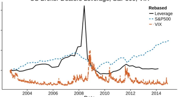
During the Great Moderation perceived volatility, as measured by the VIX index of expected future volatility, declined consistently over several years, as shown by the dotted line in Figure 1. At the same time, in a near mirror image to volatility, asset prices (as measured by the S&P500 index) and leverage of

1_{Such a constraint may arise in a number of ways. If the investor is using collateralized}

loans to fund its investments, it must maintain margin on its collateral. Alternatively, a regu-lator may impose a risk contingent capital adequacy ratio. Finally, internal risk management considerations may lead the investor to adopt a Value-at-Risk constraint. (In simple terms Value-at-Risk is a measure of how much the bank could lose with a given small probability). All of these cases effectively impose a risk contingent leverage constraint.

2_{In principle, distressed banks can reduce their leverage in two ways: they can raise more}

capital or sell assets. In practice most banks tend to do the latter, as documented in Adrian and Shin (2008).

3_{Minsky was the first author that we know of to describe the leverage cycle in qualitative}

terms. The first quantitative model is due to Geanakoplos (1997, 2003); Fostel and Geanako-plos (2008); GeanakoGeanako-plos (2010). See also the early model by Gennotte and Leland (1990), which models the destabilizing effects of leverage but does not model the cycle per se. An-other relevant model is Brunnermeier and Pedersen (2008), where the authors investigate the destabilizing feedback between funding liquidity and market liquidity. A further discussion on the destabilizing effects of margin can be found in Gorton and Metrick (2010).

1 2 3 4 2004 2006 2008 2010 2012 2014 Date Rebased v alue relativ e to 2002Q3 Rebased Leverage S&P500 VIX

US Broker Dealers Leverage, S&P500, VIX

Figure 1: The leverage of US Broker-Dealers (solid black line) compared to the S&P500 index (dashed blue line) and the VIX S&P500 (red dash-dotted line. Data is quarterly; see footnote 7.

financial institutions (as measured by the leverage of US security broker dealers) consistently increased.4 _{As financial institutions expanded their leverage their}

assets and liabilities grew correspondingly.

The Great Moderation came to a sudden and dramatic halt when the US subprime mortgage crisis began to unfold in late 2007 and the subsequent fi-nancial crisis sent asset prices into a downward spiral. As asset prices began to fall, market volatility increased. At the same time the leverage of financial institutions increased – in fact drastically so. This was due the fact that even relatively small drops in asset prices can massively increase the leverage of fi-nancial institutions that are already highly leveraged. Fifi-nancial institutions responded quickly to increased market volatility and deleveraged by a factor of 2 in the span of one quarter.

This deleveraging likely had a drastic negative impact on asset prices. Of course, many other factors affected asset prices at that time, and this evidence is only anecdotal. Nonetheless, the correlation observed between asset prices, volatility and leverage motivates the model that is developed here, which is de-signed to address the following questions: How do leveraged investors respond to changes in market prices? How are market prices affected by investors’ portfolio adjustments? How does this potential feedback loop affect the overall

dynam-4 _{It should be noted that US security broker dealers are a somewhat extreme example}

of leveraged financial institutions and are not representative for the behavior of commer-cial banks. Here we use their example to illustrate the stark correlation between leverage, volatility and asset prices in an anecdotal way. A more nuanced evaluation can be found in Adrian and Shin (2010). The data on US Security Broker Dealer Leverage, (defined as Assets/(Assets-Liabilities), is from US Federal Reserve Flow of Funds Data Package F.128 available athttp://www.federalreserve.gov/datadownload/.

ics of the financial system? Finally, what should regulators do to control this feedback loop, and how should they make an appropriate compromise between microprudential and macroprudential regulation?

Our model suggests that the underlying cause of these events might have been due to the simple combination of leverage and dynamic risk management in the style of Basel II, and that the collapse of the housing bubble might have been only the spark that happened to cause the crash. Of course the real situation was complicated and this cannot be proven, but our model makes this explanation plausible.

1.2. Review of literature on leverage cycles

There are many possible mechanisms that have been conjectured to drive leverage cycles. In the original model of Geanakoplos investor heterogeneity plays a key role: The most optimistic investors are also the most leveraged investors. The leveraged investors are hit harder by downturns, which reduces their market power, which negatively impacts average expectations and amplifies downward price movements. Many other factors have been conjectured to drive leverage cycles, including short-termism, herding and incentive distortions.5

Here we focus on the side-effects of risk management as a driver of leverage cycles. A passive investor, i.e. an investor that never rebalances his or her portfolio, iscountercyclicalin the sense that falling prices drive leverage up and vice versa. In contrast, Adrian and Shin (2008) point out that many investors, such as commercial banks, use constant leverage targets, creating a positive feedback between the demand for an asset and its return. Since falling prices increase leverage, maintaining a constant target leverage causes investors to sell into a falling market and to buy into a rising market. Such behavior is inherently destabilizing: Higher (lower) demand leads to higher (lower) prices, that further increase (reduce) demand, and so on.

Adrian and Shin (2008) document even more destabilizing behavior by in-vestors such as investment banks. These inin-vestors are actively procyclical, i.e. they lower leverage targets when prices fall and raise them when prices rise. This further amplifies the potentially destabilizing positive feedback between demand and returns. Adrian and Shin argue that this can be due to regula-tory risk management, since a risk neutral investor subject to a Value-at-Risk constraint increases her leverage when volatility is low and reduces it when volatility is high. In fact, volatility and prices cannot be disconnected. There is empirical evidence for a negative correlation between returns and volatility (Black, 1976; Christie, 1982; Nelson, 1991; Engle and Ng, 1993). This implies that when prices increase (decrease), volatility decreases (increases) and target leverage goes up (down), which results in leverage procyclicality. The fact that minimum capital requirements based on VaR are likely to result in procyclical behavior was also pointed out by Estrella (2004).

Since VaR risk management induces the procyclicality of leverage with re-spect to prices, in the following we will refer to a procyclical leverage control policyas one for which banks are required to reduce their target leverage when volatility increases, and are allowed to increase it when volatility decreases. It is important to stress that this feedback can have significant macro-economic consequences. For instance Van den Heuvel (2002) investigates the effect of cap-ital regulation on the transmission of monetary policy via bank lending, finding that leverage procylicality can lead to an amplification of monetary policy.

In contrast to the procyclical case, we will refer to acountercyclical leverage control policy as one for which banks can target a higher leverage if volatility is high, but are required to reduce their leverage when volatility is low. The rationale for such a policy is to counteract the potentially destabilizing positive feedback between demand and returns that occurs under procyclical policies. We show that an actively countercyclical policy can also be destabilizing. In fact, under a policy that is countercyclical with respect to risk, we observe in our model that the relation between returns and volatility can be reversed, and that higher (lower) volatility is associated with higher (lower) prices. Therefore, if an investor buys when volatility increases, this can further increase volatility and prices, which raises leverage targets, etc., also resulting in a positive feedback loop. The challenge for policy makers is to find a leverage control policy that avoids the Scylla and Charybdis of excessively procyclical policies on one side or excessively countercyclical policies on the other. The aim of this paper is to understand how the cyclicality of leverage control policies affects the properties of the financial system, and to seek the proper compromise between these two extremes.

It has to be stressed that the concept of cyclicality we refer to in this paper is with respect to risk, not with respect to the behavior of macroeconomic indi-cators. For example, Drehmann and Gambacorta (2012) provide counterfactual simulations showing how leverage control policies that are countercyclical with respect to the difference between the credit-to-GDP ratio and its long-run aver-age can help making the economy more stable. The focus of our paper, however, is on the circumstances in which risk control can cause financial instability, and how to make an effective tradeoff between systemic vs. individual risk.

The consequences of procyclical leverage have now been studied by many authors.6 _{The fact that feedback loops due to capital requirement constraints}

can lead to the amplification of shocks has been demonstrated, for example, by Zigrand et al. (2010), He and Krishnamurthy (2012), Thurner et al. (2010) and Adrian and Boyarchenko (2012a, 2013). Aymanns and Farmer (2014) go be-yond this by showing how leverage constraints can lead to an endogenous cycle, i.e. one in which spontaneous oscillations occur. We call this theBasel

lever-6_{See for example Danielsson et al. (2001), Danielsson et al. (2004), Adrian and Shin (2008),}

Shin (2010), Zigrand et al. (2010), Adrian et al. (2012), Tasca and Battiston (2012), Poledna et al. (2013), Adrian and Shin (2014) and Brummitt et al. (2014).

age cycle.7 _{While Adrian and Boyarchenko (2012a, 2013) study this through}

a dynamic stochastic general equilibrium model, Aymanns and Farmer (2014) consider a more stylized setting where investment decisions of households and unleveraged funds are not explicitly modeled. The latter model has the virtue of being very simple, and also of showing how under bounded rationality en-dogenous leverage cycles can occur even in a deterministic limit where there are no shocks. In this paper we modify the model of Aymanns and Farmer (2014) by adding a fundamental noise trader subject to exogenous noise, which allows us to study the tradeoff between micro and macro prudential regulation. We also present a full stability analysis.

1.3. Summary of our contribution

Our main contribution is the identification of optimal leverage control poli-cies. As in the Aymanns and Farmer model, the exponent of the relationship between perceived risk and target leverage is a free parameter. In this way it is possible to capture both procyclical and countercyclical leverage control policies in a single model. The ability to interpolate between procyclical and counter-cyclical leverage control policies in one model allows us to compare policies of different “cyclicality” and study their effectiveness in controlling leverage cycles. In order to do this it is necessary to choose a criterion for selecting the optimal policy. We believe a good policy is one that maximizes leverage at a given level of overall risk to the financial system. Maximizing leverage is desirable because this means that the capital of the financial system is put to full use in providing credit to the real economy. In fact, for reasons of convenience it is more feasible for us to minimize risk at a given leverage; this is essentially equivalent, since the average leverage can be adjusted to match any desired risk target (and the policy that is selected will be the same). We measure risk in terms of realized shortfall, i.e. the average of large losses to the financial system as a whole.

The main result of this paper is that the optimal policy depends critically on three parameters: the average leverage used by the bank; the relative size of the bank and the fundamentalist; and the amplitude of the exogenous noise. A procyclical leverage control policy such as that of Basel II is optimal when the exogenous noise is high, the volatility is strongly clustered, the bank is small and leverage is low; in the opposite limit where these conditions are not met the optimal policy is closer to constant leverage.

2. A simple model of leverage cycles

2.1. Sketch of the model

We consider a financial system composed of a leveraged investor (called a bankfor simplicity), an unleveraged fund investor, which we call the fund, and

7_{However bear in mind that this can occur even without any regulatory policy constraint,}

due to prudent risk managers who limit the risk of individual institutions in isolation while failing to properly take systemic risk into account.

a passive outside lender that provides credit as required by the bank. The bank and the fund make a choice between investing in a risky asset whose price is determined endogenously vs. a risk free asset with fixed price, which we will callcash.

We focus on risk management by assuming the bank holds the relative weight of the risky asset and cash fixed. The bank’s risk management consists of two components: First, we assume that the bank estimates the future volatility of its investment in the risky asset by using an exponential moving average of historical returns. Second, the bank uses the estimated volatility to set its desired leverage. The target can be set either by internal risk management or by externally imposed regulatory constraints: The net result is the same. If the bank is below its desired leverage, it will borrow more and use the additional funds to expand its balance sheet. Conversely, if it is above its desired leverage, it will liquidate part of its investments and pay back part of its debt.

The fund is a proxy for the rest of the financial system, i.e. the part that does not do leverage targeting. Leverage targeting creates inherently unstable dynamics, as it implies buying into rising markets and selling into falling mar-kets. Thus it is necessary have at least one other investor who plays a stabilizing role. We model the fund as a weakly fundamentalist investor whose investment decisions are perturbed by exogenous random shocks reflecting information flow or decision processes outside the scope of the model. The exogenous random shocks display clustered volatility. The fund investor and the bank interact through the market for the risky asset and the market clearing price is deter-mined by the investments of the fund and the bank.

Because of the clustered volatility, in the absence of any systemic effects, the bank should adjust its leverage to maintain a constant Value at Risk. With systemic effects this becomes more complicated, which is what this model allows us to investigate.

In addition to its portfolio management decisions, we assume that the bank tries to maintain a constant target equity. This is consistent with the empirical observation that the equity of commercial and investment banks is roughly constant over time; see Adrian and Shin (2008). In order to conserve cash flow in our model, we assume that dividends paid out by the bank when the equity exceeds the target are invested in the fund, while new capital invested in the bank when the equity is below the target is withdrawn from the fund. This prevents all the wealth from accumulating with either the bank or the fund and makes the asymptotic dynamics stationary.

Figure 2 shows a diagrammatic representation of the model. The main driver of the dynamics is the feedback loop between changes in the price of the risky asset and balance sheet adjustments: The bank reacts to price changes to maintain its capital requirements under its perception of risk; similarly the fund invests as one expect from a fundamentalist, buying when prices are below value and selling when they are above. The balance sheet adjustments of the bank and the fund determine the price, which in turn feeds back to determine their decisions.

update

risk estimate

adjust

balance sheet

bank

underleveraged

→

new borrowing

overleveraged

→

liquidate assets

detect

mispricing

update

decision

fund

asset

revaluation

regulatory

constraint

exogenous

shock

equity flow

Figure 2: Diagrammatic representation of the model: The bank and the fund interact through price formation. The bank’s demand for the risky asset depends on its estimated risk based on historical volatility and on its capital requirement. The demand of the fund consists of a mean reverting component that tends to push the price towards its fundamental value; in addition there is a random exogenous shock to the fund’s demand that has clustered volatility. Price adjustments affect the bank’s estimation of risk and the mean reverting behavior of the fund. The cash flow consistency in the model is enforced by equity flowing between the bank and the fund in equal amounts. The driver of the endogenous dynamics is the feedback loop between price changes, volatility and demand for the risky asset.

2.2. Leverage regulation

The most important ingredient of our model is the fact that the bank is subject to a capital requirement policy. The leverage ratio8 _{of the bank is}

defined as

λ(t) = Total Assets

Equity , (1)

and the capital requirement policy implies a leverage constraint of the type

λ(t) ≤ ¯λ(t), i.e. the bank is allowed a maximum leverage ¯λ(t). A cap on leverage is equivalent to the existence of a minimum capital buffer that the bank is required to keep to absorb losses. Conditional on the leverage constraint, it can be shown that the return on equity of the bank is maximized ifλ(t) = ¯λ(t) (see for instance Shin (2010)). We therefore assume that the bank always targets its maximum allowed leverage ¯λ(t).9

We assume that ¯λ(t) depends on the bank’s estimate of the volatility of the risky asset, i.e. ¯λ(t) =F(σ2_{(t)), where σ}2_{(t) is the bank’s perceived risk.}

Although nothing we do here depends on this, to gain intuition it is useful to compute the function F under the special case of a Value-at-Risk constraint with normally distributed returns. In this case the bank’s target leverage is given by (see for example Corsi et al. (2013)):

¯

λ(t) =F_VaR(σ2(t)) = 1

σ(t)Φ−1_(a)∝

1

σ(t),

where Φ is the cumulative distribution of the standard normal, a is the VaR quantile, and σ the volatility of the risky asset. Under this specification the bank increases its leverage when the volatility of the risky asset diminishes and decreases its leverage in the opposite case. Motivated by Adrian and Shin (2014), we classify leverage policies as follows:

Definition 1. A leverage policy F(σ2(t)) is procyclical if dF/dσ2 _{< 0 and}

countercyclicalifdF/dσ2_>0.10

8_{We use this definition of leverage in analogy to the Tier 1 regulatory leverage ratio (Tier}

1 capital over bank total assets). An alternative definition of the leverage ratio only considers risky assets in the numerator. Since in our model the bank holds the share of risky assets to total assets fixed, this alternative definition simply introduces a multiplicative constant into the leverage calculation and does not affect the qualitative outcome of our model.

9_{In reality banks usually keep more capital than required by regulation in order to reduce}

the cost of recapitalization or portfolio adjustments associated with violation of the minimal capital requirement. Using this perspective, Peura and Keppo (2006) explain the pattern of capital buffers observed in a sample of US commercial banks. However, note that our results remain valid even if we assume that banks hold more capital than required by the regulator. We only require that the resulting bank capital buffer responds to changes in perceived risk in a well defined way, i.e. in our model changes in the capital buffer are more important than the level of the capital buffer.

10_{This definition could be generalized for any risk measure; we use the standard deviation}

A class of leverage control policies that allows us to interpolate between procyclical and countercyclial leverage control policies is given by

¯ λ(t) =F_(α,σ2 0,b)(σ(t)) :=α(σ 2_{(t) +σ}2 0)b, (2) whereα >0,σ2

0>0 andb∈[−0.5,0.5]. We refer to αas the bank’s riskiness.

The largerαthe larger the bank’s target leverage for a given level of perceived riskσ2_(t).11 _{For the special case where returns are normal with b=−0.5 and}

σ2

0= 0,αis linked to the quantile used to measure VaR by the inverse

cumula-tive normal distribution. In the more general case where there are heavy tails or with other choices of parameters this correspondence is no longer valid. How-ever, since the variance of returns is finite, under the Chebyshev’s bound VaR is bounded by a quantity inversely proportional to the standard deviation of the return distribution, so the conjectured relationship in Equation (2) remains qualitatively correct. The relationship between α and risk remains monotonic under any sensible risk measure, and one can simply think ofαas a risk param-eter and Equation (2) as a particular choice ofF, corresponding to a volatility estimate based on historical standard deviation.

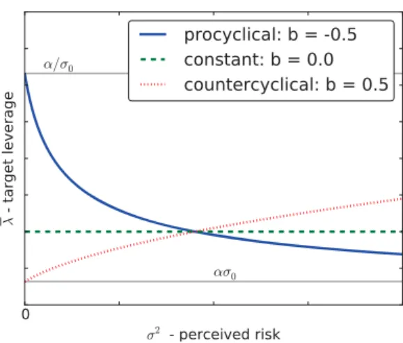
The parameter b is called the cyclicality parameter, due to the fact that

F_(α,σ2

0,b)is procyclical forb <0 and countercyclical forb >0 (see Definition 1). For procyclical policies the leverage is inversely related to risk, i.e. leverage is low when risk is high and vice versa. For countercyclical policies the opposite is true; when risk is high leverage is also high, see Figure 3. It is important to note that our definition of policy cyclicality does not refer to macroeconomic measures such the credit-to-GDP ratio or asset prices. Instead it is defined solely by the bank’s response to changes in perceived risk. In this sense the countercyclical policies proposed in this model differ from the countercyclical capital buffer proposed by the Bank of England, see FPC (2014), which keys off the credit-to-GDP ratio.

Finally, the parameter σ2

0 bounds the leverage control policy from above

for b < 0 such that F_(α,σ2

0,b) ≤ α(σ

2

0)b and from below for b > 0 such that

F_(α,σ2

0,b)≥α(σ

2

0)b. For the remainder of this paper we will restrict our analysis

to leverage control policies of the classF_(α,σ2

0,b). We illustrate the three corner cases of the above class of leverage control policies withσ₀2>0 in Figure 3. 2.3. Asset price dynamics

The bank’s target leverage ¯λ(t) at time t defines a target portfolio value ¯

A_B(t) = ¯λ(t)E_B(t), where E_B(t) is the equity of the bank. The difference

be-11 _{Note that under standard Value-at-Risk the bank’s leverage depends on the variance}

of its entire portfolio which in our model includes non risky cash holdings. Usually, the portfolio variance is computed as the inner product of the covariance matrix with the portfolio weights. In our case this implies that the portfolio variance is simplyσ2_{(t) scaled by the bank’s}

investment weight in the risky assetwB. However, since we takewBconstant throughout, the resulting risk rescaling factor can be absorbed intoαwithout loss of generality. Therefore, we makeF_(α,σ2

Figure 3: Illustration of target leverage as a function of perceived risk based on Equation (2) withσ₀2 >0. Continuous blue line: procyclical policy withb =−0.5. Dashed green line: constant leverage policy withb = 0. Dotted red line: countercyclical policy withb= 0.5. Continuous grey lines show relation toσ0.

tween the target portfolio and the current portfolio then determines the change of the balance sheet ΔB(t) required for the bank to achieve its target leverage:

• If ΔB(t)> 0, the bank will borrow ΔB(t) and invest this amount into the risky and the risk free asset according the bank’s portfolio weights.

• If ΔB(t)< 0, the bank will liquidate part of its portfolio and pay back ΔB(t) of its liabilities.

The evolution of the fund’s portfolio weight in the risky asset depends on the asset’s price relative to a constant fundamental valueμ, and also on random innovations. The fund investor therefore combines two economic mechanisms: (1) The constant fundamental value means that the price of the risky asset is ultimately anchored on the performance of unmodeled macro-economic condi-tions, which we assume are effectively constant over the length of one run of our model. (2) We allow random innovations in the portfolio weight that reflect exogenous shocks.

We assume that the fund invests a fraction w_F(t) of its total assets in the risky asset, and that the time evolution ofw_F(t) follows a mean reverting process with a GARCH(1,1) noise term. Thus, the fundamentalist investor provides a source of time varying exogenous volatility to the model. It is important that the exogenous volatility is time varying as this motivates the need for microprudential leverage control: To minimize risk, the bank must estimate the expected future volatility and adjust its leverage accordingly.

Given the aggregate demand of the bank and the fund, and assuming for simplicity that there is a supply of exactly one unit of the risky asset that is

infinitely divisible, the price of the risky asset is determined through market clearing by equating demand and supply.

2.4. Time evolution

The model evolves in discrete time-steps of lengthτ. We make this a free parameter so that the model has well-defined dynamics in the continuum limit

τ →0, which is useful for calibration. At each time-step the bank and the fund update their balance sheets as follows:

• The bank updates its historically-based estimate of future volatility and computes its new target leverage accordingly. Volatility estimation is done using an exponential moving average with an approach similar to Risk-Metrics (see Longerstaey (1996));

• The bank pays dividends or raises capital to reach its target equityE;

• The bank determines how many shares of the risky asset it needs to trade to reach its target leverage;

• At the same time, the fundamentalist fund submits its demand for the risky asset;

• The market clearing price for the risky asset is computed and trades oc-cur.12

2.5. The model as a dynamical system

The dynamics of our model can be described as an iterated map for the state variablex(t), defined as

x(t) = [σ2(t), w_F(t), p(t), n(t), L_B(t), p(t)]T, (3) whereσis the historical estimation of the volatility of the risky asset;w_F is the fraction of wealth invested by the fund in the risky asset; p the current price of the risky asset; nthe share of the risky asset owned by the bank; L_B the liabilities of the bank; andpis the lagged price of the asset, i.e. the price at the previous time step. A detailed derivation of the model is presented in Appendix

12_{It is important to note that the decision concerning equity and investment adjustments is}

taken before the current trading price of the risky asset is revealed. We therefore assume that the bank uses the price of the previous time step as a proxy for the expected trading price, and acts accordingly. This assumption of myopic expectations marks a significant departure of our model from the general equilibrium setting of Adrian and Boyarchenko (2012b) and Adrian and Boyarchenko (2013), but it is common in the literature on heterogeneous agents in economics (see for instance Hommes (2006)).

A. Here we simply present the model and provide some basic intuition. Let us introduce the following definitions:

Bank assets A_B(t) =p(t)n(t)/w_B,

Target leverage λ¯(t) =α(σ2(t) +σ₀2)b,

Balance sheet adjustment ΔB(t) =τ θ(¯λ(t)(A_B(t)−L_B(t))−A_B(t)),

Equity redistribution κ_B(t) =−κ_F(t) =τ η(E−(A_B(t)−L_B(t))),

Bank cash c_B(t) = (1−w_B)n(t)p(t)/w_B+κ_B(t),

Fund cash c_F(t) = (1−w_F(t))(1−n(t))p(t)/w_F(t) +κ_F(t).

The parameters θ and η determine how aggressive the bank is in reaching its targets for leverage and equity respectively (i.e. the bank aims at reaching the targets on time horizons of the order 1/θ and 1/η).

The model can be written as a dynamical system in the form

x(t+τ) =g(x(t)), (4) where the functiongis the following 6-dimensional map:

σ2(t+τ) = (1−τ δ)σ2(t) +τ δ log p(t) p(t) t_VaR τ 2 , (5a) w_F(t+τ) =w_F(t) + wF(t) p(t) τ ρ(μ−p(t)) +√τ sξ(t), (5b) p(t+τ) = wB(cB(t) + ΔB(t)) +wF(t+τ)cF(t) 1−w_Bn(t)−(1−n(t))w_F(t+τ) , (5c) n(t+τ) = wB(n(t)p(t+τ) +cB(t) + ΔB(t)) p(t+τ) , (5d) L_B(t+τ) =L_B(t) + ΔB(t), (5e) p(t+τ) =p(t). (5f) Each of these equations can be understood as follows:

(a) The expected volatility σ2 _{of the risky asset is updated through an}

expo-nential moving average. The parameter τ δ ∈ (0,1) defines the length of the time-window over which the historical estimation is performed, while the parameter t_VaR represents the time-horizon used by the bank in the calculation of VaR.

(b) The adjustment of the fund’s risky asset portfolio weightw_Fdrives the price towards the fundamental valueμ, with an adjustment rateτ ρ∈(0,1). The demand of the fund also depends on exogenous noise, which is assumed to be a normal random variableξ(t) with amplitudes(t)≥0. The amplitude varies in time so that the variable χ(t) =s(t)ξ(t) follows a GARCH(1,1) process. The factors ofτ guarantee the correct scaling asτ →0.

(c) The market clears. c_F(t) andc_B(t) are the amount of cash held respectively by the fund and the bank.

Symbol Description Default Unit

Bank τ Time step 0.1 year

δ Memory for volatility estimation 0.5 year−1

t_VaR Horizon for VaR calculation 0.1 year

σ2

0 Risk offset 10−6 1

b Cyclicality of leverage control −0.5 (v) 1

α Risk level 0.075 (v) 1

E Bank’s equity target 2.27 (v) 1

w_B Bank’s weight for risky asset 0.3 (v) 1

θ Balance sheet adjustment speed 9.5 (v) year−1

η Equity redistribution speed 10 year−1

Fund μ Fundamental value 25 1

ρ Mean reversion 0.1 year−1

GARCH a₀ Baseline return variance 10−3 ₁

a₁ Error autoregressive term 0.016 1

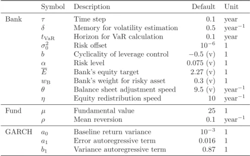
b₁ Variance autoregressive term 0.87 1 Table 1: Overview of parameters for the numerical model solution. Values marked with (v) indicate that they are subject to change from their default values; “1” indicates that the parameter is dimensionless.

(d) The bank ownership of the risky assetn(t+ 1) adjusts according to market clearing.

(e) Bank liabilities are updated to account for the change ΔB(t) in the asset side of the balance sheet.

(f) The lagged price variablep(t) is required to complete the state vector, and make the map a first order dynamical system of the form given in Equation (4).

3. Examples of leverage cycles

In order to explore the dynamical behavior of the model we solve it numeri-cally. For now we will only consider leverage control policies that are procyclical; in particular we chooseb=−0.5 throughout this section, corresponding to the case of risk management under VaR.

3.1. Model calibration

While this model is too stylized to be fully calibrated, approximate values for some key parameters can be obtained. This then allows us to test the realism of some of the properties of the model. In the following we will briefly discuss the choice and effect of these key parameters, including the timescale of the risk estimation, the balance sheet adjustment speeds and bank riskiness. A full list of parameters is provided in Table 1.

Timescale parameters

We have carefully constructed the dynamical system so that it reaches a continuum limit as τ → 0. For computational efficiency we choose τ to be the largest possible value with behavior similar to that in the continuum limit, which results in a time step ofτ = 0.1 years. As long asτ is this size or smaller the results change very little.

The parameterδ sets the timescale for the exponential moving average used to estimate volatility, and is the most important determinant of the overall timescale of the dynamics. The characteristic time for the moving average is

t_δ = 1/δ.13 _{According to the RiskMetrics approach Longerstaey (1996), the}

typical timescale used by market practitioners is t_δ ≈ 2 years. We thus have the luxury of being able to calibrate this parameter from “first principles”. We therefore setδ= 0.5 year−1, corresponding to a two year timescale, and keep it fixed throughout.

Another timescale parameter ist_VaR, the time horizon over which returns are computed for regulatory purposes. In practice, the timescale for the regulatory capital requirements varies depending on the liquidity of the asset portfolio and ranges from days to years. A good rule of thumb is to chooset_VaRroughly equal to the time needed to unwind the portfolio. We assume t_VaR= τ = 0.1 years, i.e. a little more than a month.

The parameters θ and η define how aggressive the bank is in reaching its target for leverage and equity. Our default assumption is that the bank tries to meet its target on a timescale of about one time step of the dynamics, and so unless otherwise stated, in the following we set θ = 9.5 year−1 _{and η =}

10 year−1_{. This ensures that the bank’s realized leverage is always close to its}

target. We will vary the parameterθand discuss how it affects the stability of the dynamics in Section 4.3.

Market power of the bank

The dynamics of this model depend on the competition between the stabi-lizing properties of the fundamentalist and the destabistabi-lizing properties of the bank. Thus to understand the parameters and their effect on the dynamics is it useful to understand how they influence the market power of the bank, which is roughly speaking the product of the leverageλand the relative size of the banking sectorR. To get a feeling of this, we show in Equation (A.10) in the appendix that at the fixed point equilibrium the parametersE,w_B,w_F,μ,

σ₀, andα all jointly determine the fraction of the risky assetR owned by the bank. Note that the numerical values chosen for the target equity E and the fundamental priceμ are arbitrary – only their ratio is important. We choose the values of the above parameters in order to produce the desired value of

R (though we often vary αindependently). Note that the bank represents all

13 _{The contribution to the moving average of a squared return y(t) observed at time t}

is y(t+ Δt) = (1−τδ)Δt/τy(t) at timet+ Δt. We define the typical time tδ such that y(t+tδ)/y(t) = 1/e. Thustδ=−τ/log[1−τδ]≈1/δforτδ1.

investors with leverage targets, and the set of institutions with a comparable Value-at-Risk based leverage constraint14_{is larger than the banking sector.}

The other key parameter affecting the stability of the model is the bank riskinessα. Increasingαincreases both the bank’s market power and its default risk. Note thatαis also related tot_VaRby the fact that, all else equal, increasing the timescale over which the risk is measured corresponds to taking more risk. (Increasingαusually increases leverage, though as discussed in footnote 18 this is not always true). The bank’s portfolio weight w_B for the risky asset has a similar effect to the bank’s equity targetE.15 _{Increasing any of these parameters}

increases the bank’s market power.

In our calibration we choose a particular level of bank riskinessα and the relative size of the bank and the fund to match two basic properties of the run up and the subsequent collapse of leverage and asset prices during global financial crisis in 2008/2009. First, we seek a peak to trough ratio in the price of the risky asset of roughly 2. Second, we target a period of oscillation of roughly ten years. Matching these calibration targets comes at the price of achieving realistic levels of bank leverage in our simulations. Given our choice for α we obtain levels of bank leverage of around 6. This is below typically observed levels of leverage of around 20. The fact that we cannot calibrate our model to match several calibration targets simultaneously is a clear weakness of the model, but is not surprising given its simplicity. It should also be noted that due to hedging banks may be able to achieve levels of risk that are much lower than that of a single bare asset as we model here, and this may explain the discrepancy in leverage.

Finally, we pick parameters for the fund GARCH process a₀, a₁ and b₁

in order to achieve a randomly perturbed asset price path that still follows a leverage cycle roughly as observed in Figure 1.

3.2. Overview of model dynamics

We now build some intuition about the model dynamics. First, consider the extreme case where E → 0, i.e. where the market power of the bank is negligible so that the price dynamics are dominated by the fund. This is the purely microprudential case where the bank’s actions have no significant effect on the market and the only source of volatility is exogenous. In this case (s >0) we expect the price to perform a mean reverting random walk around the fundamental priceμ. In the deterministic case, i.e. s= 0, the fund updates its portfolio weight until p(t) = μ, i.e. until the price has converged to the fundamental price and the system settles to a fixed point equilibrium.

WhenEis large enough that the bank has a significant impact on the price process the dynamics are less straightforward. We refer to this scenario as the macroprudential case. Suppose, for example, that there is a negative shock in

14_{In principle the constraint can be either imposed by a regulator, creditors or internal risk}

management.

the investment of the fund. This negative shock will lead to an increase in the perceived riskσ2_{(t). Under a procyclical leverage control policy an increase in}

perceived risk causes a decline in the bank’s leverage constraint. As a conse-quence the bank will have to deleverage in the time step following the negative shock, i.e. ΔB(t)<0. If the bank decreases its position and it has non-negligible market impact, the price will drop for ΔB(t)<0 ceteris paribus. This is clear from Equation A.7 in the appendix. Thus an initial negative shock can be am-plified by the bank’s deleveraging response. This destabilizing feedback loop is a key ingredient for what is to come and distinguishes risk management in the macroprudential case from the microprudential case. In the macropruden-tial case the bank’s risk management affects the system’s state and introduces endogenous volatility on top of exogenous volatility.

To illustrate the dynamics of the model we will investigate the following four scenarios:

(i) Deterministic, microprudential: E= 10−5 _{ands= 0.}

(ii) Deterministic, macroprudential: E= 2.27 ands= 0. (iii) Stochastic, microprudential: E= 10−5_{ands >0.}

(iv) Stochastic, macroprudential: E= 2.27 ands >0.

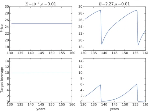
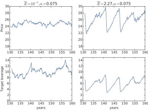
Unless otherwise stated all parameters are as specified in Table 1. The first two cases are for the deterministic limit with s = 0, which is useful to gain intuition. The last two cases are with more realistic levels of exogenous noise. We summarize our results for scenarios (i) and (ii) in Figure 4 and for scenarios (iii) and (iv) in Figure 5.

The microprudential scenarios (i) and (iii) behave as expected: In the de-terministic limit the systemic simply settles into a fixed point with prices equal to fundamental values. When there is exogenous noise the system makes ex-cursions away from the fixed point but never drifts far away from it, and the dynamics remain relatively simple.

In contrast the macroprudential scenarios (ii) and (iv) display large oscil-lations both in leverage and price. We refer to this oscillation as the Basel leverage cycle. Surprisingly, the oscillations occur even in the deterministic limit, i.e. without any external shocks. During the cycle the price and leverage slowly rise and then suddenly fall, with a period of about Δt≈15 years in the deterministic case.

In the stochastic case we observe a period of about Δt ≈ 10 years. This is roughly on the order of magnitude of the period of the Great Moderation and the subsequent financial crisis. Note that the period of oscillation depends strongly on the risk estimation horizont_δ, but this is set to two years based on behavioral data.16

16_{In fact, the period is roughly proportional to 1/tδ. The period becomes large for very}

low values ofδτ and then declines as the risk estimation horizon is increased – for the range of τδthe variation of the period ranges over roughly two orders of magnitude. The period also depends on the values ofη,tVaR,θ,wBandα. AsηortVaRare increased the period increases.

Figure 4: Time series of price and leverage in the deterministic case. Left panel: scenario (i) – microprudential, the fund dominates the bank (E= 10−5), i.e. the bank has no significant market impact. In this case the system goes to a fixed point equilibrium where the leverage and price of the risky asset remain constant. Right panel: scenario (i) – macroprudential, the bank has significant market impact (E= 2.27). In this case the bank’s risk management leads to persistent oscillations in leverage and price of the risky asset with a time period of roughly 15 years.

Figure 5: Time series of price and leverage in the stochastic case. Left panel: scenario (iii) – microprudential, the fund dominates the bank (E= 10−5), i.e. the bank has no significant market impact. In this case the price is driven by the fund’s trading activity and performs a mean reverting random walk around the fundamental valueμ= 25. Right panel: scenario (iv) – macroprudential, the bank has significant market impact (E= 2.27). In this case the bank’s risk management leads to irregular oscillations in leverage and price of the risky asset that are similar to the deterministic case.

The oscillations have the following economic interpretation: Suppose we begin at about t = 140 years in the left panel of Figure 4, with leverage low, perceived risk high, and prices low but increasing. The perceived risk slowly decreases as the memory of the past crisis fades. From a mechanical point of view this is due to the smoothing action of the exponential moving average. As the moving average is updated on each timestep, the volatility σ2 _decreases;

this causes the leverage to increase, and the bank buys more shares to meet its increased leverage target. The change in price is lower than the current historical average, so on the next step the volatilityσ2_{drops, driving the leverage higher.}

As the leverage becomes very high the system becomes increasingly fragile. In the phase space the system approaches a hyperbolic fixed point where the leverage is so large that that a crash occurs. The downward crash ultimately comes to an end by the increasingly heavy investment of the fundamentalist fund. After the crash volatility is high and leverage is low, and the cycle repeats itself.

The fragility that drives the crashes comes from the fact that at high levels of leverage a small increase in risk is sufficient to cause a drastic tightening of the leverage constraint. This intuition can be made precise by comparing the derivative of the leverage control policy for high vs. low leverage; for convenience we takeσ2

0 1.17 The result is that

dF_(α,σ2 0,−0.5) dσ2_(t) (σ 2_{(t)) =} −0.5/σ₀ 0 , forσ2_{(t)→0 ∧ σ}2 0 1 0 , forσ2_{(t)→ ∞ ∧ σ}2 0 1

In the high leverage limit, i.e. when the perceived risk is small, the sensitivity of the leverage target F to variations in risk tends to infinity. In contrast the sensitivity is zero in the opposite limit where leverage is low and perceived risk is large. Thus increasing leverage of the banking system has a two-fold destabilizing effect: It can make the dynamics unstable and lead to chaos, but it also makes it more sensitive to shocks, which can result in sudden deleveraging. The leverage cycles are not strictly periodic due to the fact that the oscil-lations are chaotic. This becomes clearer by plotting the dynamics in phase space and then taking a Poincar´e section, as illustrated in Figure 6. The phase plot makes the cyclical structure clearer; the 3D representation shows how the ownership of the risky asset varies during the course of the leverage cycle (left panel). The Poincar´e section is constructed by plotting ownership vs. per-ceived risk every time the trajectory crosses the hyper-planep(t) = 20 with the price increasing (right panel). The Poincar´e section shows the characteristic fractal structure, and shows the stretching and folding that makes the

dynam-Asθ,αandwBare increased, i.e. as the system moves to a more unstable regime, the period declines. However, for these parameters the variation in the period over the parameter range is only on roughly one order of magnitude. The period of oscillation is robust to changes in wF.

17_{Forb <0 the parameterσ0 imposes a cap on the target leverage; larger values forσ}2 0

0 0.01 0.02 0.03 0.04 0.05 0.06 0 0.05 0.1 0.15 0.2 18 20 22 24 26 28 30 Perceived Risk Ownership Price ï

Figure 6: Left panel: Three dimensional phase plot of the system’s attractor when there is a deterministic leverage cycle. Right panel: A Poincar´e section is constructed by recording values for the bank ownership of the risky asset (y-axis) and the perceived risk (x-axis) when-ever the price is increasing andp(t) = 20, repeating for 106 time steps. This exhibits the characteristic stretching and folding associated with chaotic dynamics.

ics chaotic. The fact that these dynamics are chaotic is confirmed in the next section, where we do a stability analysis and compute the Lyapunov exponent. In summary, depending on the choice of parameters, the model either goes to a fixed point (scenario (ii)) or shows chaotic irregular cycles (scenarios (i) and (iii)). As expected the dynamics become more complicated when noise is added, but the essence of the Basel leverage cycle persists even in the zero noise limit.

4. Determinants of model stability

4.1. Deterministic case

In the deterministic case the standard tools of linear stability analysis can be used to characterize the boundary between the fixed point equilibrium and leverage cycles. In this section we will use this to characterize the behavior of the system as the risk parameterαand the cyclicality parameter bare varied. We begin by studying the deterministic case, where we can compute things analytically, and then present numerical results for the stochastic case. The details of the stability analysis are presented in Appendix A.

The system has a unique fixed point equilibriumx∗, given by

x∗= (σ2∗, w∗_F, p∗, n∗, L∗_B, p∗) = (0, w_F(0), μ,1 μασ 2b 0 EwB,(ασ20b−1)E, μ). (6)

This corresponds to a leverageλ∗and relative size of bank to fundR_c(x∗), given by λ∗=ασ₀2b, R(x∗) = A ∗ B A∗_F = λ∗E_B∗ (1−n∗)p∗/w_F∗. (7)

At the equilibrium x∗ the price is constant at its fundamental value and the bank is at its target leverage. The stability of the equilibrium depends on the parameters. Regime (i) observed in the numerical simulations of the previous section corresponds to the stable case. In this case, regardless of initial condi-tions, the system will asymptotically settle into the fixed pointx∗. In contrast, when the fixed pointx∗is unstable there are two possibilities. One is that there is a leverage cycle, in which the dynamics are locally unstable but exist on a chaotic attractor that is globally stable; the other is that the system is globally unstable, in which case the price either becomes infinite or goes to zero.

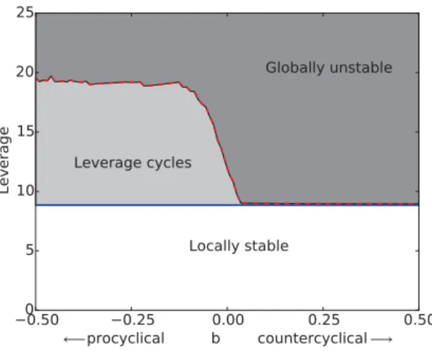
In Figure 7 we show the results of varying the risk parameter α and the cyclicality parameterb. The risk parameterαprovides the natural way to vary the risk of the bank, but the realized risk for a given α depends on parame-ters due to other factors such as changes in volatility. For diagnostic purposes leverage is a better measure.18 Figure 7 shows each of the three regimes, cor-responding to the stable equilibrium, leverage cycles or global instability, as a function of the leverage and the cyclicality parameter b. The boundary where the fixed point equilibrium becomes unstable is computed analytically based on the leverageλ∗_c where the modulus of the leading eigenvalue is one. The bound-ary for globally unstable behavior is more difficult to compute as it requires numerical simulation.

This diagram reveals several interesting results. As expected, for low lever-age the system is stable and for higher leverlever-age it is unstable. Somewhat sur-prisingly, the critical leverageλ∗_c is independent of b, and consequently the size of the regime with the stable equilibrium is unaffected by whether the lever-age control is procyclical or countercyclical. In the procyclical regime there is a substantial area of parameter space with leverage cycles. For the counter-cyclical regime, in contrast, there is only a small regime with leverage cycles. Throughout most of the parameter range the system makes a direct transition from the stable fixed point equilibrium to global instability. The instability is not surprising: In the countercyclical regime there is an unstable feedback loop in which increasing leverage drives increasing prices and increasing volatility, which further increases the leverage. Thus for high leverage there are unstable regimes for both pro- and countercyclical behavior, but the instability is even worse in the countercyclical regime.

4.2. Stability when there is exogenous noise

In the case where there is exogenous noise we can only measure the stability numerically. This is done by computing the largest Lyapunov exponent of the dynamics. The Lyapunov exponents are a generalization of eigenvalues that apply to trajectories that are more complicated than fixed points. The leading

18_{Whileαtends to increase leverage, when the leverage control policy is procyclical the}

behavior is not always monotonic. This is because increasingαtends to increase volatility, but increasing volatility drives the target leverage down, so the two effects compete with each other.

Figure 7: A bifurcation diagram showing the three regimes in the deterministic case. The risk parameterαand the cyclicality parameterbare varied while holding the other parameters constant at the value in Table 1. The white region corresponds to a stable fixed point equi-librium, the light gray region to leverage cycles and the dark gray region to global instability. The blue line corresponds to the critical leverageλ∗

c in Equation 7 at the critical valueαc where the fixed point becomes unstable.

Lyapunov exponent measures the average rate at which the separation between two nearby points changes in time – when the dynamics are locally stable nearby points converge exponentially and the leading Lyapunov exponent is negative, and when they are locally unstable nearby points diverge exponentially and the leading Lyapunov exponent is positive. The Lyapunov exponent is a property of a trajectory, but for dissipative systems such as ours, it is also a property of the attractor. A negative Lyapunov exponent implies a fixed point, and a positive Lyapunov exponent implies a chaotic attractor. As expected, in the deterministic case we observe that leverage cycles have a positive leading Lyapunov exponent, confirming that the dynamics are chaotic.

It is also possible to compute Lyapunov exponents for stochastic dynamics. To understand the basic idea of how this is done, imagine two realizations of the dynamics with the same sequence of random shocks, but starting at slightly dif-ferent initial conditions, see Crutchfield et al. (1982). Because the random noise is the same in both cases, it is possible to follow two infinitesimally separated points and measure the rate at which they separate. If the leading Lyapunov exponent is positive this means that the dynamics will strongly amplify the noise.

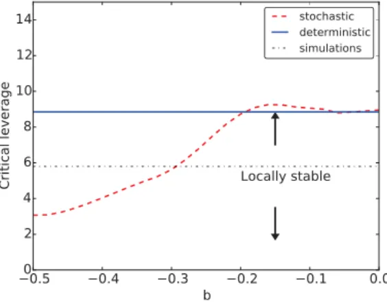
We compare the stability for the stochastic and deterministic cases in Figure 8. This is done for the procyclical case only, since the direct transition from a fixed point to global instability in the countercyclical case complicates numerical work (and the countercyclical case is less relevant). In the stochastic case the critical leverage is computed as the time average of the target leverage when

Figure 8: A comparison of stability when the dynamics are deterministic vs. stochastic for the procyclical region (b < 0). As in the previous figure, the critical leverage λ∗_c for the deterministic case is shown as a blue line. The dashed red line shows the parameter value where the dynamics become unstable as measured by the leading Lyapunov exponent; note the transition to chaos occurs at a much lower leverage. The gray line shows the average target leverage obtained in the simulation, which is roughly independent ofb.

the Lyapunov exponent becomes positive. Interestingly, the critical leverage in the stochastic case first starts below the deterministic critical leverage and then approaches it asbis increased. This indicates that for strongly procyclical leverage control policies noise destabilizes the system. Somewhat surprisingly, the average leverage observed in the simulations is independent ofb.

The most interesting conclusion from comparing the stochastic and deter-ministic cases is that when the dynamics are strongly procyclical (i.e. for

−0.5 < b < −0.2) the noise significantly lowers the stability threshold. In contrast, for larger values of b >−0.2 there is little difference in the stability threshold in the two cases. This indicates that the dynamics becomes more sta-ble when the leverage control policy is close to constant leverage. This, together with the fact that in the countercyclical regime the system goes straight from stability to global instability, suggests that intermediate values of cyclicality (nearer to constant leverage) are likely to be most stable.

4.3. Slower adjustment leads to greater stability

The bank’s balance sheet adjustment speedθhas a strong effect on stability with interesting regulatory implications. Intuitively, decreasing the adjustment speed should make the system more stable. To take an extreme case, in the limit

τ θ →0, the bank would hold its balance sheet constant regardless of changes in perceived risk. This would eliminate the feedback loop between asset prices, perceived risk and investment. Even when θ > 0, decreasing the adjustment

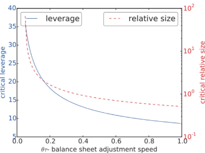
Figure 9: Critical leverageλ∗_c (solid blue line, left vertical axis) and the critical value of the relative size of the bank to the fundRc(x∗) (dashed red line, right vertical axis) as a function of the balance sheet adjustment speedθτ. Other parameters are as in Table 1. The stability of the financial system can be dramatically improved by lowering the adjustment speed.

speed should have a stabilizing effect.19

To test this we study how the critical leverageλ∗_c and critical relative size

R_c(x∗) depend on the adjustment speed θτ (we varyθ and hold τ constant). The relationship is shown in Figure 9, where the critical leverage is shown on the left vertical axis and the critical relative size on the right vertical axis. As expected, both the critical leverage (left axis, continuous line) and critical relative size of the bank (right axis, dashed line), decrease dramatically as θτ

increases. This suggests that it is possible to dramatically improve the stability of the financial system if institutions adjust to their leverage targets slowly. Similarly, this illustrates the dangers of mark-to-market accounting, which can cause balance-sheet adjustments to be too rapid .

5. Leverage control policies

What is the optimal leverage control policy? The mere fact that the endoge-nous oscillations of prices and volatility depend on the cyclicality parameterb, as shown in Figure 7, suggests that some policies are better than others. In

19_{We have considered the case where the bank increases its leverage quicker than it decreases}

it. We have done this introducing an asymmetry in the parameterθthat controls the speed of leverage adjustement, i.e. introducing a parameterθ+for the speed of levering up and a parameterθ−for the speed of deleveraging. By allowing such asymmetric specification, we find that the dynamics becomes more stable asθ− is reduced. The qualitative behavior of the system, namely the existence of stable, locally unstable and globally unstable regimes, is preserved.

this section we introduce a procedure for scoring policies and search for the best policy within the family that we have defined. We find that the optimal policy depends on parameters of the model, and in particular on the market power of banks in relation to the rest of the financial system. As the market power of banks increases the optimal policy becomes increasingly countercyclical, and in the limit where the banks play a large role in determining prices it approaches constant leverage.

5.1. Criterion for optimality

We define an optimal leverage control policy as one that maximizes leverage for a given level of risk. Maximizing leverage is desirable because it means that, for a given level of capital, banks