Efficient Euclidean Distance Transform
Using Perpendicular Bisector Segmentation
∗†Jun Wang and Ying Tan
‡Key Laboratory of Machine Perception (Ministry of Education), Peking University
Department of Machine Intelligence, School of EECS, Peking University, Beijing, P.R. China
[email protected] [email protected]
Abstract
In this paper, we propose an efficient algorithm for com-puting the Euclidean distance transform of two-dimensional binary image, called PBEDT (Perpendicular Bisector Eu-clidean Distance Transform). PBEDT is a two-stage inde-pendent scan algorithm. In the first stage, PBEDT com-putes the distance from each point to its closest feature point in the same column using one time column-wise scan. In the second stage, PBEDT computes the distance transfor-m for each point by row with intertransfor-mediate results of the previous stage. By using the geometric properties of the perpendicular bisector, PBEDT directly computes the seg-mentation by feature points for each row and each segment corresponding to one feature point. Furthermore, by us-ing integer arithmetic to avoid time consumus-ing float opera-tions, PBEDT still achieves exact results. All these methods reduce the computational complexity significantly. Conse-quently, an efficient and exact linear time Euclidean dis-tance transform algorithm is implemented. Detailed com-parison with state-of-the-art linear time Euclidean distance transform algorithms shows that PBEDT is the fastest on most cases, and also the most stable one with respect to im-age contents.
1. Introduction
Given a binary image, whose elements have only the val-ue 0 — background (feature) pixels — and 1 — feature (background) pixels, its distance transform computes the distance for each pixel between that pixel and the feature pixel closest to it [21]. Distance transform (DT) algorithms ∗This work is supported by National Natural Science Foundation of China (NSFC), under grant number 60875080 and 60673020, and partly supported by the National High Technology Research and Development Program of China (863 Program), with grant number 2007AA01Z453.
†The source code of PBEDT is available on http://cil.pku.edu.cn/algorithm/distancetransform/
‡Ying Tan is the corresponding author.
are excellent tools for a variety of applications, such as im-age processing, computer vision, pattern recognition, mor-phological filtering and robotics, etc. [9][19][21]. In prac-tice, several distance metrics, such as the city-block (L1), the chessboard (L∞), the octagonal and the Euclidean
met-ric, are all used for different situations. One of the most natural and appropriate one of these is the Euclidean met-ric, which is radially symmetric and virtually invariant to rotation [1][9][16], and used in many applications. Howev-er, theDT in exact Euclidean metric, called EDT, is time consuming.
Intuitionally, treated as a global operation, EDT can be computed by using an exhaustively brute-force search-ing algorithm: for each pixel of the image, calculate the distance between that pixel and each feature pix-el. This requires O(N2) time (N is the number of image pixels) [1][16]. Numerous algorithms have been proposed to restrict the searching for the closest fea-ture pixel in order to realize a fast EDT computa-tion. In terms of searching mode, all these algorithm-s can be roughly claalgorithm-salgorithm-sified into three categoriealgorithm-s, ordered propagation[2][20], raster scan [5][20][21] and independen-t scan [1][6][12][13][15][16][22]. However, so far independen-there is no algorithm which can compute the EDT with good effi-ciency and good precision [9]. Some extensive surveys are introduced in [2] and [9]. They indicate that an efficient EDT should be based on obtaining feature pixels informa-tion from limited region, and should avoid global search-ing. Although many of these algorithms are of liner time complexity, some are not stable when the image content is changed or have a large constant term [2][9].
In this paper, we propose an efficient algorithm for com-puting the Euclidean distance transform of two-dimensional binary image, called PBEDT (Perpendicular Bisector Eu-clidean Distance Transform). PBEDT is a two-stage inde-pendent scan algorithm. In the first stage, PBEDT computes the distance from each point to its closest feature point in the same column using one time column-wise scan. In the second stage, PBEDT computes the distance transform for
each point by row with intermediate results of the previous stage. By using the geometric properties of the perpendicu-lar bisector, PBEDT directly computes the segmentation by feature points for each row and each segment corresponding to one feature point. Furthermore, by using integer arith-metic to avoid time consuming float operations, PBEDT still achieves exact results. The remainder of this paper is organized as follows. In Section 2, the detail of PBEDT is introduced. The refined implementation of the proposed algorithm is presented in Section 3. Experiments of com-parison with state-of-the-art algorithms on variant feature objects and in-depth discussion are reported in Section 4. Finally, Section 5 gives the concluding remarks of this pa-per.
2. PBEDT by perpendicular bisector
segmen-tation
2.1. Preliminary
As usual, this algorithm takes a n by m binary image as the input and outputs a distance transform, usually in squared distance. LetIdenote the point set of the image,
Ir denote the points in row r, and FI denote the set of feature pixels. (Generally, let uppercase letter denote point set and lower case letter denote point.) Letf(u)denote the closest feature point ofu, andk · kis the Euclidean metric:
f(u) = arg
v∈FI
minku−vk, u∈I. (1)
Thus, the distance transform of imageI can be computed by:
DT(u) =ku−f(u)k2, u∈I (2) The feature points in the columncare denoted by :
Cc={v|v.x=c, v∈FI},0≤c < n (3) PBEDT is a two-stage independent scan algorithm. In the first stage, it computes the closest feature points for each row. Then in the second stage, it computes the distance of each point to its closest feature point by row [1][16].
2.2. First stage
For rowr, given two feature pointsu, v ∈Cc, ifku.y−
rk<kv.y−rk, then any point in rowris closer touthan to v. If∃u∀v ∈ Cc,ku.y−rk ≤ kv.y−rk,uis called r’s closest feature point in column c. All closest feature points in columns of rowrare denoted bySr
g, and|Sgr| ≤n. Therefore,f(u)is rewriten as:
f(u) = arg
v∈Sr g
minku−vk, u∈Ir. (4)
2.3. Second stage
In this stage, we give an effective method to compute (4). LetSr
f denote the closest feature points of rowr, and
Sr f ⊆Sgr.
Sfr= [
u∈Ir
f(u) (5)
Let points inSrg andSrf are increasingly ordered by x coordinate. LetPtrdenote the set of points in rowrwhose closest feature point is t, called t’s region of influence in rowr.
Ptr={v|f(v) =t, v∈Ir}, t∈Sgr (6) Ift ∈ Sfr, thenPtr 6= ∅; otherwise, Ptr = ∅. Hence,
Sfr=Sgr− {u|Pur=∅, u∈Srg}. 0 2 4 6 8 0 2 4 6 8 u v B uv p(c uv r ,r) 0 2 4 6 8 0 2 4 6 8 c u v w p v
Figure 1. The perpendicular bisector ofuandvintersects row r.
We take advantage of the geometrical property of per-pendicular bisector to verify the points whose region of in-fluence is empty. LetBuvdenote the perpendicular bisector ofuandv(Fig.1). Buv is the set of points which have e-qual distance touandv. Consequently, the points located at theuside ofBuv are closer touthan tov. Letcruv de-note the x coordinate of the intersection ofBuv with row
r. Hence, pointp(cr
uv, r)(Fig.1) is the separation point of
Pr
u andPvr (Pur =6 ∅, Pvr 6= ∅, u.x < v.x), and we assign
p ∈ Pr
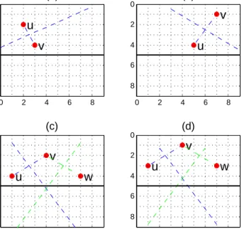
u, p 6∈ Pvr. Givenu.x < v.x, the points in Ir at the left ofcruv are closer to uthan to v. The situations in Fig.2(a)(b) clearly indicate a point’s region of influence in rowris empty.
Ifcr
uv > crvw(u, v, w ∈ Sgr), then Pvr = ∅(Fig.2(d)). Next,uandwwill be compared with other points inSr
g. If
cr
uv < crvw(u, v, w∈Sgr), thenPvr6=∅(Fig.2(c)). Howev-er, point vwill not be compared with all the points inSr
g, since the region of influence has some special properties: Property 1. The points in set Pr
t are continuous in
x-coordinate, or,@v{v|u.x≤v.x≤w.x, u,w∈Ptr,v6∈Ptr}.
(Ifvexists, thens=f(v). Thus,Bstintersects rowr
be-tweenuand v, and betweenvandw, too. This violates the fact that two lines only intersects at most once.)
0 2 4 6 8 0 2 4 6 8
u
v
(a) 0 2 4 6 8 0 2 4 6 8u
v
(b) 0 2 4 6 8 0 2 4 6 8u
v
w
(c) 0 2 4 6 8 0 2 4 6 8u
v
w
(d)Figure 2. Four situations when a point is added inS1. (a)Pur=∅; (b)Pvr=∅; (c)Pur6=∅; (d)Pvr=∅; Moreover, Property 2. Ifu, v ∈ Sr f, u.x < v.x, then s.x ≤ t.x , ∀s∈Pr u and∀t∈Pvr.
Therefore, if the points inSr
gat the left of pointvare all verified, then none of them is closer to the right ofcr
uvthan
v(Property.1, Property.2). ComputeS1
S1andScare stacks. Initially,S1andScare both empty.
whileS0is not empty
withdraw the lowest pointwfromS0; ifS1is empty
push(S1, w); push(Sc, 0);
else
vis top ofS1andcruvis top ofSc; calculatecr vwwithvand w;
pop(S1), pop(Sc), add w back to the
f ront of S0, when crvw < cruv;
pop(S1), pop(Sc), push(S1, w),
push(Sc, crvw), when crvw=cruv;
push(S1, w), push(Sc, crvw),
when cr
vw> cruvand crvw< cols; returnS1;
Consequently, we give an algorithm COMPUTES1to ob-tainSr
ffromS r
g. LetS1andScbe stack structures. Initially, letS0 =Sgr, andS1 =∅. Points are moved fromS0toS1
one by one. If an added point results in pointpofS1whose region of influence in rowris empty, thenpshould be re-moved fromS1. WhenS1is empty, we push 0 intoScas the first intersection point. In the next loop, we use the newly added pointwand the stack top ofS1 pointv to compute
cr
vw, and comparecrvwto the stack top ofSc. The 0 at the bottom of stack labels the edge of the processing row.
Next, we proveS1=Sfr.
Theorem 1. S1=Sfr
Proof:This proof has two steps: 1. Pvr=∅,∀v∈Sgr−S1;
In the algorithm COMPUTES1, the points of S0 are moved to S1 one by one, and only the point whose region of influence onris empty is removed fromS1. Therefore,Pr
v =∅,∀v∈Sgr−S1. 2. Pr
v 6=∅,∀v∈S1;
Following algorithm COMPUTES1, each pointv (ex-cept the endpoints) and its adjacent points u, w
(u, v, x ∈ S1 and u.x < v.x < w.x) have two separation position cr
uv and crvw. cruv < crvw, thus
cruv< Pvr.x≤crvw.
The left endpointvand its adjacent pointwhave a sep-aration positioncr
vw. crvw >0, thus0< Pvr.x≤crvw. (The right end point is in a similar way.) Therefore,
Pr
v 6=∅,∀v∈S1. Therefore,S1=Srf.
Thus, each point in Ir is compared with two adja-cent points in Sfr at most to get its closest feature point (Property.1, Property.2). By processing each row with COMPUTES1, we get the closest feature point for each point of I. Thus, we calculate the EDT by (2).
3. Implementation of PBEDT
In this section, we introduce the implementation of PBEDT.
3.1. First stage algorithm
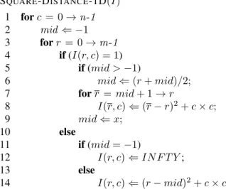
Different from former independent scan algorithm-s [1][16], which compute the algorithm-squared dialgorithm-stance in 1-D by twice scan, in the first stage, we compute the rela-tive squared distance between the closest feature points in column and the left end point of each row by a for-ward scan with back propagation. IN F T Y used in SQUARE-DISTANCE-1D(I) is an integer bigger than the squared diagonal distance of the image.
SQUARE-DISTANCE-1D(I) 1 forc = 0→n-1 2 mid ⇐ −1 3 forr = 0→m-1 4 if(I(r, c) = 1) 5 if(mid >−1) 6 mid⇐(r+mid)/2; 7 forr =mid+ 1→r 8 I(r, c)⇐(r−r)2+c×c; 9 mid⇐x; 10 else 11 if(mid=−1) 12 I(r, c)⇐IN F T Y; 13 else 14 I(r, c)⇐(r−mid)2+c×c;
3.2. Second stage algorithm
We implement the second stage algorithm introduced by COMPUTES1in an effective way.
3.2.1 Calculate the intersection points
Buvintersects rowrat(cruv, r), thusku−(cruv, r)k=kv−
(cr
uv, r)k(Fig.1), and we obtaincruv:
cr
uv= {(v.x)2−(u.x)2−2×r×(v.y−u.y)
+(v.y−r)2−(u.y−r)2}/{2×(v.x−u.x)}
We use the relative distance to replace the y coordinate,
¯
y=y−r, thencr
uvcan be simplified as:
cruv= ((v.x)
2+ (v.y)2)−((u.x)2+ (u.y)2)
2(v.x−u.x) ; Moreover, let du= (u.x)2+ (u.y¯)2 (7) , then cruv= dv−du 2(v.x−u.x). (8)
This calculation can be organized as a function
(Intersection), which only has 1 division , 1 multiplication,
and 2 substraction.
Intersection(ux, vx, du, dv)
return(dv−du)/(2∗(vx−ux));
From (7),duis the squared distance ofuto the left most point of row r which can be computed in the first stage (SQUARE-DISTANCE-1D).
3.2.2 Integer calculation
We use integer division to replace the float division in (8). The integer division abandons the decimal and keep the in-teger, which is faster but not always accurate. In our algo-rithm, we use the efficiency of integer arithmetic and keep the accuracy meanwhile. Fig.3 shows two different situa-tions, butcr
uv =crvw = 4in every situation by integer divi-sion. In both of situations, we assign point p(4,5) is close to the leftmost point of this triple —u, since the point coordi-nates ofIare all integers. Even ifBuv andBvw all inter-sect at point p(4,5), the assignment is valid. Therefore, an equivalent integer division will be more efficient than float division. 0 2 4 6 8 0 2 4 6 8
u
v
w
c (a) 0 2 4 6 8 0 2 4 6 8u
v
w
c (b)Figure 3. Different situations of assigning same closer feature point: (a)cr
uv> crvw; (b)cruv< crvw
Negative values between two integers will be rounded to the lager integer (-0.9 will be rounded to 0), while positive values in between two integers will be rounded to the small-er integsmall-er (5.9 will be rounded to 5). Thsmall-erefore, we use -1 to label the left edge of the processing row while we use 0 in COMPUTES1. Moreover, we prejudge the sign ofcr
uv before calculating it, which promotes the execution speed. In (8),vx < uxis known, thus the sign ofcruvis relative to
(dv−du).
Therefore,Intersectionis rewritten as:
Intersection-INT(ux, vx, du, dv)
if(dv > du)
return(dv−du)/(2∗(vx−ux)); else
return -2;
3.2.3 Euclidean distance computation
We also useduwhich comes from (7) in the distance com-putation. Givenuis a point on rowr(u.y=r) andvis the closest feature point ofu, then
ku−vk2 = (u.x−v.x)2+ (u.y−v.y)2
= (u.x)2−2(u.x)(v.x) + (v.x)2+ (v.y)2
This can be organized as a function, which only has one addition, one substraction and two multiplications.
Distance(ux, vx, dv)
returnux∗(ux−vx∗2) +dv;
3.2.4 Second stage algorithm
Based on the technical details above, we give the second stage algorithm (SQUARE-DISTANCE-2D).
SQUARE-DISTANCE-2D(I) 1 forr= 0tom−1 2 stack c⇐ ∅;stack cx ⇐ ∅; 3 stack g ⇐ ∅;p⇐ −1 4 forc = 0ton−1 5 if(I(r, c)< IN F T Y) 6 while(TRUE) 7 if(p≥0) 8 cx⇐Intersection-INT(stack c[p], c,stack g[p],abs(I(r, c))) 9 if(cx=stack cx[p]) 10 p⇐p−1; 11 else if(cx < stack cx[p]) 12 p⇐p−1; 13 continue; 14 else if(cx≥(n−1)) 15 break; 16 else 17 cx⇐ −1; 18 p⇐p+ 1; 19 stack c[p]⇐c; 20 stack cx[p]⇐cx; 21 stack g[p]⇐I(r, c); 22 break; 23 if(p <0) 24 returnFALSE; 25 c⇐0; 26 fork= 0top 27 if(k=p) 28 cx⇐n−1; 29 else 30 cx⇐stack cx[k+ 1]; 31 while(c≤cx) 32 I(r, c)⇐Distance(c, stack c[k], stack g[k]); 33 c⇐c+ 1;
3.3. Computational complexity
We discuss the computational complexity of PBEDT: • The time complexity of PBEDT isO(N)times.
1. In the first stage, SQUARE-DISTANCE-1D takes O(N) time, since it scans forward once and prop-agates backward at most 0.5N. Thus, each ele-ment is accessed no more than twice, leading to an average number of 1.5 access times per ele-ment (computational complexity ofO(N)). 2. In the second stage, SQUARE-DISTANCE-2D
processes m rows one by one. There are two pro-cesses for each row, one computesstackcxand the other computes squared distance.
In process one, |Sr
g| ≤ n, and each point in
Sr
g can only be added to stackc once. Each point instackc can only be removed once, and
|stackc| ≤ n . Hence, these adding and re-moving operations are executed at most 2n times. Thus, process one takesO(n)time.
Process two computes the distance between each point w in row r and w’s closest feature point compute once, and takesO(n)time.
Hence, in the second stage, SQUARE-DISTANCE-2D takes O(N) (O(m ∗ n)) times.
• The space requirement of PBEDT is very low. In each stage, PBEDT recycles the memory of input image. In the second stage, PBEDT need a tempo-rary memory whose size is 3n to storestackc,stackcx,
stackg.
4. Experiments and discussion
To evaluate its performance, PBEDT was compared with state-of-the-art EDT algorithms, such as Maurer et al.’s [16], Saito and Toriwaki’s [22], Cuisenaire and Macq’s [4], Lotufo and Zampirolli’s [6], Meijster’s [17] and Felzenszwalb et al.’s [10]. In order to improve readability, these algorithms are abbreviated as MAU-RER2003, SAITO1994, CUISENAIRE, LOTUFOZAM-PIROLLI, MEIJSTER, FELZENSZWALB, respectively. Felzenszwalb et al. give the implementation of their algo-rithm [11], and other algoalgo-rithms are implemented by Fabbri et al. [8].
The tests were performed on a computer with an Intel Core2 Duo 2.53GHz processor, 2GB RAM, Ubuntu Linux OS with kernel v2.6.31. All algorithms are implemented in ANSI C/C++, and built by GCC v4.1.1. The performance of PBEDT was measured with images over a wide range of sizes and contents, as Fabbri et al. recommends in [9].
Comparing the outputs of PBEDT to those of other al-gorithms, no difference has been observed from all these tests. Additional tests with thousands of randomly gener-ated images varying in width and number of feature points also indicate the correctness of our algorithm.
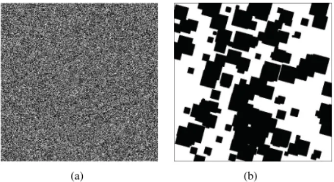
(a) (b)
Figure 4. Randomly generated sample images. (a) Random points, feature pixel proportion: 40%, size: 500×500; (b) Random squares, feature pixel proportion: 15%, square angle: 15◦, size: 500×500
(a) (b)
Figure 5. Test image Lenna. (a) Original image; (b) Edge image of Lenna
The following images are chosen for precisely analysis: 1. Random points. The image size varies from 100×
100, 500×500, ..., to 4000×4000 with randomly generated feature points where the number of feature points comprises 1%, 10%, ..., 90%, and 99% of the image. One sample is shown in Fig. 4(a). This test provides an idea of the performance of the algorithms relative to the number of feature pixels [9][16]. 2. Random squares. These images are generated by
ran-domly choosing the centers and sizes of black squares rotated byθ∈[0,90]. The squares are filled and plot-ted into the image until the black pixels add up to a percentage value p. One sample is shown in Fig. 4(b). This test is based on a synthetic image having more similarity to real images with some orientation [7][9]. 3. Special feature contents:
• A feature square located at the corner of an im-age. In this case, EDT produces the largest and s-mallest possible distances for a given image size: diagonal and 1, respectively [9][16].
• Binary images of real objects. The edge image from the Lenna image obtained by thresholding
the response of an edge detector is used, as shown in Fig. 5(b). Lenna is chosen since it has been universally used as an impartial benchmark for image analysis algorithms [9].
• A white disk inscribed in the image. It is a per-fect test for exactness, since the Voronoi diagram of the pixels along a circle is very regular in the continuous plane, however, the discrete Voronoi regions in this case are irregular, specially near the center of the disk [3][9][22].
• Half-filled image. This is the worst case of the brute-force algorithm, and Maurer2003 also suf-fers a setback in this test [9].
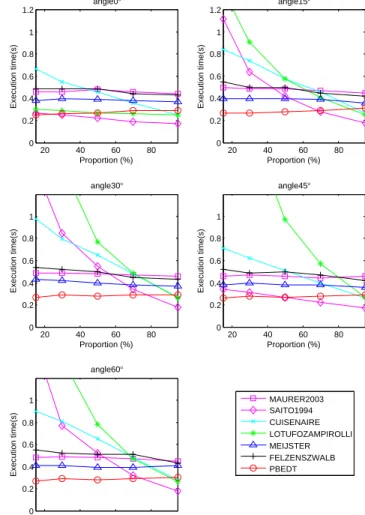
As shown in Fig. 6 and Fig. 7, PBEDT is more sta-ble than other algorithms with different proportions of fea-ture pixels, and it is faster than MAURER2003, MEIJSTER and FELZENSZWALB at all parameter settings used, faster than SAITO1994 and LOTUFOZAMPIROLLI at small pro-portion feature pixels, slower than CUSENAIRE only at very large proportion of feature points. Besides, PBEDT is more stable than others with different slant angle of ran-dom squares. SAITO1994 and LOTUFOZAMPIROLLI are faster than PBEDT when slant angle is 0 or 90, but s-lower when other angles are used. Only when the pro-portion of feature pixels is higher than 70%, SAITO1994, CUSENAIRE and LOTUFOZAMPIROLLI are faster than PBEDT at every slant angel. Fig. 8(a) shows that PBEDT is the fastest with the test of edge image of Lenna at all sizes. Fig. 8(b) shows that PBEDT is the fastest in all feature con-tents.
In all these tests, PBEDT shows excellent performance. It is the fastest in most cases, and the most stable in terms of image contents. Neither the number of feature pix-els nor the orientation of content objects can affect it-s performance. It is faster than MAURER2003, MEI-JSTER and FELZENSZWALB in all cases, and faster than SAITO1994, LOTUFOZAMPIROLLI and CUISENAIRE in most cases. SAITO1994 and LOTUFOZAMPIROLLI are seriously affected by the orientation of feature objects, which show poor performance in most of angles. Moreover, their performance varies with different proportion of feature pixels. Table.1 shows the mean execution time on random-ly generated squares with various feature point proportions and slant angels at size3000×3000. Obviously, of all al-gorithms, PBEDT is the fastest one.
5. Conclusion
We have introduced a two-stage independent scan algo-rithm PBEDT, which is simpler than previous works: use partial Voronoi diagram [1][16] or lower-envelop of parabo-las [10][14][17][22]. The time complexity of PBEDT is linear in the number of image points with a small constant
0 20 40 60 80 0 0.2 0.4 0.6 0.8 1 1.2 proportion15% Execution time(s) Angle (°) 0 20 40 60 80 0 0.2 0.4 0.6 0.8 1 1.2 proportion30% Execution time(s) Angle (°) 0 20 40 60 80 0 0.2 0.4 0.6 0.8 1 proportion50% Execution time(s) Angle (°) 0 20 40 60 80 0 0.2 0.4 0.6 0.8 1 proportion70% Execution time(s) Angle (°) 0 20 40 60 80 0 0.2 0.4 0.6 0.8 1 proportion95% Execution time(s) Angle (°) MAURER2003 SAITO1994 CUISENAIRE LOTUFOZAMPIROLLI MEIJSTER FELZENSZWALB PBEDT
Figure 6. Execution time for random squares images with varying feature point proportion, size3000×3000, slant angle varied from 0 to 90.
Algorithms Average Comparison with
time(s) PBEDT (%) MAURER2003 0.469 168.2% SAITO1994 0.441 158.0% CUISENAIRE 0.547 196.0% LOTUFOZAMPIROLLI 0.802 287.3% MEIJSTER 0.391 139.9% FELZENSZWALB 0.483 173.2% PBEDT 0.279 100%
Table 1. Comparison of average execution time for randomly gen-erated squares images.
term and the memory requirement is very low. Compared with other state-of-the-art algorithms, PBEDT is the fastest in most cases, and also the most stable one with respect to image contents. The main innovations of this
algorith-20 40 60 80 0 0.2 0.4 0.6 0.8 1 1.2 angle0° Execution time(s) Proportion (%) 20 40 60 80 0 0.2 0.4 0.6 0.8 1 1.2 angle15° Execution time(s) Proportion (%) 20 40 60 80 0 0.2 0.4 0.6 0.8 1 angle30° Execution time(s) Proportion (%) 20 40 60 80 0 0.2 0.4 0.6 0.8 1 angle45° Execution time(s) Proportion (%) 20 40 60 80 0 0.2 0.4 0.6 0.8 1 angle60° Execution time(s) Proportion (%) MAURER2003 SAITO1994 CUISENAIRE LOTUFOZAMPIROLLI MEIJSTER FELZENSZWALB PBEDT
Figure 7. Execution time for random squares images with varying slant angle, size3000×3000, feature points proportion ranged from 15% to 95%.
m are: the geometric property of perpendicular bisector is used to compute the segmentation of rows directly; the inte-ger arithmetic is used to avoid time consuming float opera-tions and still keeps exactness. All these innovaopera-tions reduce the computational complexity significantly. A parallel ver-sion of PBEDT can be easily implemented [18][21]. This algorithm can also be extended to three or higher dimen-sional binary images. Currently, we are evaluating the n-D version of this algorithm. Results will be published in a more elaborate paper which is currently in preparation.
References
[1] H. Breu, J. Gil, D. Kirkpatrick, and M. Werman. Linear time euclidean distance transform algorithms.IEEE Transactions on Pattern Analysis and Machine Intelligence, 17(5):529– 533, 1995.
10000 1500 2000 2500 3000 3500 4000 0.5
1 1.5 2
2.5 Test with edge image of Lenna
Execution time(s) Image width MAURER2003 SAITO1994 CUISENAIRE LOTUFOZAMPIROLLI MEIJSTER FELZENSZWALB PBEDT (a)
Top−left0 Bottom−right Lenna White disk Half filled 0.01
0.02 0.03 0.04 0.05
Test with special content images
Execution time(s) Image content MAURER2003 SAITO1994 CUISENAIRE LOTUFOZAMPIROLLI MEIJSTER FELZENSZWALB PBEDT (b)
Figure 8. Test results. (a) Results with Lenna edge images of ranged size; (b) Results with images of special features, size 500×500.
and applications to medical image processing. PhD thesis, Louvain-la-Neuve, Belgium, 1999.
[3] O. Cuisenaire and B. Macq. Fast and exact signed euclidean distance transformation with linear complexity. InICASSP ’99: Proceedings of the Acoustics, Speech, and Signal Pro-cessing, 1999, IEEE International Conference, pages 3293– 3296, Washington, DC, USA, 1999. IEEE Computer Society. [4] O. Cuisenaire and B. M. Macq. Fast euclidean distance transformation by propagation using multiple neighborhood-s. Computer Vision and Image Understanding, 76(2):163– 172, 1999.
[5] P.-E. Danielsson. Euclidean distance mapping. Computer Vision, Graphics, and Image Processing, 14:227–248, 1980. [6] R. de Alencar Lotufo and F. A. Zampirolli. Fast multidimen-sional parallel euclidean distance transform based on math-ematical morphology. InSIBGRAPI, pages 100–105. IEEE Computer Society, 2001.
[7] H. Eggers. Two fast euclidean distance transformations in z2based on sufficient propagation.Computer Vision and Im-age Understanding, 69(1):106–116, 1998.
[8] R. Fabbri, L. da Fontoura Costa, J. C. Torelli, and O. M. Bruno. Complete results of the benchmark between exact edt algorithms. ”http://distance.sourceforge. net”, 2006.
[9] R. Fabbri, L. da Fontoura Costa, J. C. Torelli, and O. M. Bruno. 2d euclidean distance transform algorithms: A com-parative survey.ACM Comput. Surv., 40(1), 2008.
[10] P. F. Felzenszwalb and D. P. Huttenlocher. Distance trans-forms of sampled functions. Technical report, Cornell Com-puting and Information Science, September 2004.
[11] P. F. Felzenszwalb and D. P. Huttenlocher. Distance trans-forms of sampled functions (program).http://people. cs.uchicago.edu/˜pff/dt/, 2004.
[12] M. L. Gavrilova and M. H. Alsuwaiyel. Two algorithms for computing the euclidean distance transform. Int. J. Image Graphics, pages 635–645, 2001.
[13] W. H. Hesselink and J. B. T. M. Roerdink. Euclidean skele-tons of digital image and volume data in linear time by the integer medial axis transform. IEEE Transactions on Pat-tern Analysis and Machine Intelligence, 30(12):2204–2217, 2008.
[14] T. Hirata. A unified linear-time algorithm for computing dis-tance maps. Inf. Process. Lett., 58(3):129–133, 1996. [15] Y. Lucet. New sequential exact euclidean distance transform
algorithms based on convex analysis.Image Vision Comput., 27(1-2):37–44, 2009.
[16] J. Maurer, R. Qi, and V. Raghavan. A linear time algorithm for computing exact euclidean distance transforms of bina-ry images in arbitrabina-ry dimensions. IEEE Transactions on Pattern Analysis and Machine Intelligence, 25(2):265–270, 2003.
[17] A. Meijster, J. B. T. M. Roerdink, and W. H. Hesselink. A general algorithm for computing distance transforms in lin-ear time. Computational Imaging and Vision, 18(8):331– 340, 2000.
[18] M. Miyazawa, P. Zeng, N. Iso, and T. Hirata. A systolic al-gorithm for euclidean distance transform.IEEE Transactions on Pattern Analysis and Machine Intelligence, 28(7):1127– 1134, 2006.
[19] D. W. Paglieroni. Distance transforms: Properties and ma-chine vision applications.CVGIP: Graphical Model and Im-age Processing, 54(1):56–74, 1992.
[20] I. Ragnemalm. Neighborhoods for distance transforma-tions using ordered propagation. CVGIP: Image Underst., 56(3):399–409, 1992.
[21] A. Rosenfeld and J. L. Pfaltz. Sequential operations in digital picture processing.J. ACM, 13:471–494, 1966.
[22] T. Saito and J. ichiro Toriwaki. New algorithms for euclidean distance transformation of an n-dimensional digitized picture with applications. Pattern Recognition, 27(11):1551–1565, 1994.