AGENT BASED SOLUTION OF SYSTEM DYNAMICS
SIMULATION MODELING: A CASE OF RICE STOCK BY
THE NATIONAL LOGISTIC AGENCY OF INDONESIA
1TOGAR ALAM NAPITUPULU
1
Senior Lecturer, Graduate School of Management Information Systems, Bina Nusantara University, Jakarta, Indonesia
ABSTRACT
Because of its trategic role in the economy of Indonesia, managing trading of rice nationwide has been assigned as one of the main function of the State Owned Company, BULOG. In helping to manage this commidity, a system dynamics model was built. Agent based model can also be built to facilitate decision making activities in rice economy. It is shown and argued that both modeling approach would generate the same result. It is further argued that agent based model could be more powerful and general to capture a more complex structure and dynamics. Furthermore, it enable construction of models in the absence of the knowledge about the global interdependencies at aggregate level.
Keywords: System Dynamics Modeling, Agent Based Modeling, Government Rice Stock Policy
1. INTRODUCTION
Cause and effect relationship among elements and sub-systems of the stock and price of rice system is complex and could in turn, after affecting other elements, have an effect upon itself through feed-back loop. In the presence of such feed-back loop, the behaviour of the system over time could be counter intuitive that it is usually be best studied using systems dynamics framework. When the induvidual members of the system, called agents, and their interrelationship with each other and their environment is important in determining emergencies in the system and the behaviour of the system globally then it is argued that the system is better studied using agent-based simulation model. On the otherhand if the system can be explained in aggregate term without the necessity of generating the aggregate behaviour through the study of individual agents, system dynamics framework might be more than enough. In this study, a prototype model of the system dynamic of stock and price of rice is developed. The Model can be utilized to predict the impacts of economic and non-economic policies on both stock and price of rice. Specifically the impact of random production of paddy on stock and price of rice were presented. A framework of developing an agent-based solution to the same problem is presented based on the developed system dynamic model prototype.
Why rice? Rice is a strategic commodity in Indonesia, not only because it contributes to inflation determinant that has significant effect on the nation’s economy, but it also has significant role in social and political stability of the country as it is a main staple food for the majority of the population. A slight disturbances in accessability and affordability of the population on rice have shown staggaring impact on economic and social stability which in turn hamper political stability. Historically, the overthrowned of the Former presidents Sukarno and Suharto regime stongly related to rice resillience issue.
During Suharto era, rice is one among the nine commodities that is controlled directly by a state owned company, i.e., the National Logistic Company of Indonesia, called “Badan Urusan Logistik” (BULOG). By law, the compay is given power to have monopoly power in trading the nine commodities. This includes importation,
distribution, procurement, etc. Instruments available to BULOG include price determination (ceiling price, floor price and procurement price), and establishment of national rice stocks, hence, the importance of controlling stocks.
2. THE MODELING FRAMEWORK
information-feedback characteristics of industrial activity to show how organizational structure, amplification (in policies), and time delays (in decisions and actions) interact to influence the success of the enterprise” (Forrester 1958 and 1961). Real world systems are represented in aggregate terms of stocks, flows between these stocks, and information that determines the values of the flows. Therefore it is the aggregate view in the process of abstraction that become characteristic of system dynamics, which is in the process, usually the system behavior is described in a number of interacting feedback loops, balancing or reinforcing, and delay structures.
In Agent Based simulation modeling agents are essentially decentralized. They have their behaviour at individual level, interact among themselves and their environment, and the global behavior emerges as a result of these individuals interactions, each following its own behavior rules, living together in some environment and communicating with each other and with the environment. Therefore, it is basically a bottom-up modeling as opposed to top-down modeling of system dynamics.
In the system dynamics modeling, we will be basically following the framework devloped by Roberts (1983). In this framework, it is suggested to first define the problem or to formulate problem statement that basically cimposed of (1) the owner of the problem where all aspects of the problem should be based on their perspective, (2) the time horizon, again from the owner’s perspective, (3) reference mode, i.e., emerges patterns in the system in the time horizon that are considered as problem that need to be resolved for instance through simulation, and (4) policy choice that need to be excersise in the simulation. The second step is to develop a causal and feed-back loop diagram of the variables that reflect the cause and effect relationship in the system. The formulation of this causal and feed-back loop would also set the system boundary that reflect the wholeness of the system. The third step is to develop the stock and flow diagram, composed of stocks, flows, and auxiliary (information) variables including the parameters and formulas that determine the relationships among all variables. This is the System Dynamic model of the problem or The Model. Further, The Model should be tested agaist data and once it is considered reliable, it can now be used in simulating the policy choices.
As for Agent-based modeling, a framework devoloped by Borshchev & Filippov (2004). In this framework, behaviour of agents is represented by
statecharts enabling the capturing of the different state of the agents, transitions between them, events that trigger those transitions, timing, and actions that the agent makes during its lifetime.
3. THE SYSTEM DYNAMICS OF RICE
From discussion with BULOG, i.e., the owner of the system, it was found that the system composed of two systems, the national sub-system and the BULOG level sub-sub-system. Variables were identified which are : Market Rice Stock (stok Beras Pasar), BULOG Rice Stock (Stok Beras BULOG), Rice Supply (Supply beras), Rice demand (Permintaan Beras), Rice Consumption (Konsumsi beras), Rice Price (Harga Beras), Market Operation (Operasi Pasar), Rice Procurement (Pengadaan Beras), Rice Production (Produksi Beras), Paddy Production (Produksi Padi), Population (Penduduk), Population Growth (Pertumbuhan Penduduk), Per-capita Rice Consumption (Konsumsi Beras Per-Jiwa), and Conversion Factor (Faktor Konversi).
Increases in rice production implies increases in rice supply and this in turn would raise market rice stock. Similarly, rice production itself is affected by increase in paddy production with positive relationship. On the demand side, demand increase reduces market stock. On the other hand, rice consumption would increase rice demand. Rice consumption is determined by population and per-capita consumption of rice in a positive manner.
Harga Beras- Stok Beras
Permintaan Beras
-Stok Beras Bulog Pengadaan Beras
+
-Operasi Pasar
-+ +
-HPP +
Produksi Beras +
Produksi Padi
+
Faktor Konversi +
+
Konsumsi Beras
Penduduk Konsumsi Beras
Per Orang + +
-Figure 1. BULOG Stock Causal Loop Diagram
The next step in the model building is to develop stock-flow diagram of the system. Based on the causal loop diagram (Figure 1), there are two stocks identified in the system representing two sub-systems, i.e., the BULOG rice stock sub-system and the national stock sub-system.
The Market Rice Stock (Stok Beras Pasar) is filled by flow variable Rice Supply (Supply Beras) and depleted with a rate determined by a flow variable Rice Demand (Permintaan Beras). This is shown in Figure 2 below.
? Stok Beras Pasar ?
[image:3.595.88.285.107.298.2]Supply Beras Permintaan Beras
Figure 2. Stock-Flow Diagram, National
Rice Supply is determined by rice production which in turn is dependent on paddy production multiplied by conversion factor of 0.55. During simulation the conversion factor can be set as parameter and can be alterd if the simulation wishes to study its impact. In this study, paddy production is set based on the historical production trend with the following trend equation:
Y = 42828375 + 884665.4 T ... (1) Where Y is paddy production and T represents year, with 1998 as T = 1. In addition to this trend, at any particular time or year, paddy production also is added a random component based on the standard deviation and a random number between minus 1 to positive 1, to make paddy production random along the trend.
Now the rice consumption that depleted the market stock is determined by population size and the per-capita rice consumption. The population itself is a stock variable accumulated from year to year with a yearly grow of population, which is population growth rate multiplied by the stock variable population. Population growth rate is parameter that can be altered later in simulation experimentation.
Formula for per-capita rice consumption it is assumed that consumption affected by rice price with the following formula, derived from elasticity formula:
Current per-capita consumption = EXP [price demand elasticity * LN(rice price/normal price)] * previous period consumption Or,
Per-capita rice consumption (ton/yr/person) = Price change effect * Normal per-capita rice consumption per year
Normal per-capita rice consumption per year is set to equal to 130 kg/yr/person.
Furthermore, rice price is determined by the following equation,
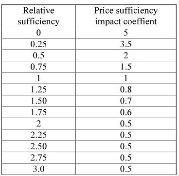
Rice price (IDR/ton) = Price Sufficiency impact coefficient * Normal price (IDR/ton)
Where price sufficiency impact coefficient is determined using the following Table 1.
Table 1. Suffiency and Price Sufficiency Impact
Relative sufficiency
Price sufficiency impact coeffient
0 5
0.25 3.5
0.5 2
0.75 1.5
1 1
1.25 0.8 1.50 0.7 1.75 0.6
2 0.5
[image:3.595.96.274.474.508.2] [image:3.595.310.494.524.705.2]Market Rice Stock
Supply Beras
Paddy Production
Conversion Factor
Rice Demand
Rice Production
Rice Consumption
Population
Population Grow th
Population Rate of Grow th Per Capita Rice
Consumption
Normal Per Capita Rice Consumption Average Rice
Demand
Smoothing Period Sufficiency Ration
Normal Suffiency Ratio
Relative Sufficiency
Sufficiency Impact Coeffient on Rice
Rice Price
Price Effect on Consumption
Normal Price of Rice Consumption Price
Elasticity Switch Button
Step Function Production
Random Production
BULOG Rice Stock
Market Operation Rice Procurement
Operation Policy Military Need
Eastern Need
Price Support Percent of Market
Stock for Support
Rice Price
Normal Price of Rice
Procurement Target Procurement Price
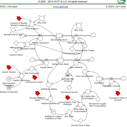
[image:4.595.88.512.93.516.2]Rice Price
Figure 3. The Complete System Dynamics Model of BULOG Rice Stock
Relative sufficiency is a ratio between Sufficiency Ratio and Normal sufficiency Ratio. For example, Relative sufficiency is equal 25 % (0.25), i.e., the ability of market stock of rice to fulfill demand is only 25 % of the normal ability, then from Table 1 then Price will increase by 3.5 times. Normal sufficiency ration is defined to be the ability of the market stock to fulfill one year demand, while the sufficiency ratio is defined to be the ratio between market stock divided by three period smoothing average of demand. This is also assumed that we introduce delay of information of three periods
from having information of changes in price to the decision of demanding rice of three months where the latest month was given the highest weight.
Assuming a 2 % population growth rate, the normal sufficiency ratio of 1 year, rice conversion of 55.22 %, normal rice price of IDR 7300/kg, per capita rice consumption of 130 kg/capita/year, rice production of 31,200,000 tons/yr in 2012, the result of the simulation are as follows:
01 Ja n 1990 01 Ja n 2000 01 Ja n 2010 25.000.000
30.000.000 35.000.000 40.000.000 ton
M
a
rk
e
t
S
to
c
k
01 Jan 1990 01 Ja n 2000 01 Ja n 2010 6.000.000
7.000.000 8.000.000 rp/ton
R
ic
e
P
ri
c
e
Price Elasticity of Consumption
-1,5 -1,0 -0,5 0,0
Population Growth Rate
0,0 0,5 1,0 1,5 2,0 2,5 3,0 %/yr
01 Ja n 1990 01 Ja n 2000 01 Ja n 2010 50.000.000
60.000.000 70.000.000 80.000.000 ton/yr
P
a
d
d
y
P
ro
d
u
c
ti
o
n
Paddy Produc tion Sc enario Random
Step Func tion
Market Support Scenario (% Market stock)
0 2 4 6 8 10
%/yr
01 Ja n 1990 01 Ja n 2000 01 Ja n 2010 2.000.000
2.500.000 3.000.000 ton
B
U
L
OG
R
ic
e
s
to
c
k
Figure 4. Simulation Results With Random Paddy Production Along The Trend
4. THE AGENT BASED MODEL OF RICE
An agent could be company, person, customer, country, or biological entity. In our example here, it appears to be that there is no suitable agent to represent. However, this should not be the case. The produce could be represented as agent such as rice, eventhough there might not be any tangible behaviour of such an agent. Even appears to be
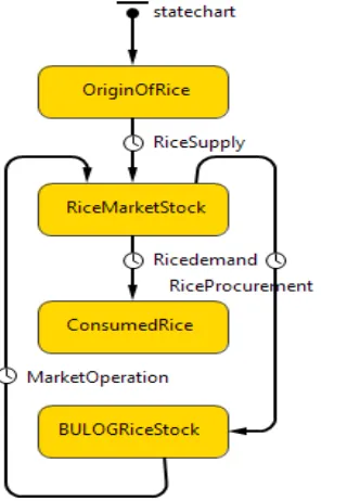
define produce rice as agent having behaviour of changing state from prior to its existence while being planted or produced by farmers to become stocks in the market as state one. Then later being consumed by the population as state two, or procured by BULOG to establish their stock. Further, the stock established by BULOG will be released in the form of market operation back to the market stock in order to stabilize the price in the market and may be to make rice available in the case of emergency, etc., according to the function given to the agency (BULOG). Therefore we need to create four states representing the behavoiur of the agents as in the following Figure 5. Correspodingly, we create four transition states explaining the rules of transition from state to state. These transitions are RiceSupply, RiceDemand, RiceProcurement, and MarketOperation. The formulas and specification for each of this transition will be followed from the system dynamics model. Now the output of the simulation that need to be monitored would be the nunber of agents (in this case rice) in each state at any particular time of the simulation experiments. Because of lack of tools available to facilitate this modeling, we will not be running this model. However, as can be seen from the explanation, we should be able to get the same results as the system dynamics model.
[image:6.595.95.261.468.699.2]Figure 5. State Chart of the Agent Based Model
5. CONCLUSIONS AND IMPLICATIONS
It can be concluded from this paper that system dynamics model can modeled using agent-based modeling and will generate the same results. The questions would be what would be the advantages of having agent based model instead of system dynamics model. As stated by Borshchev & Filippov, “Agent Based approach is more general and powerful because it enables to capture more
complex structures and dynamics. The other
important advantage is that it provides for construction of models in the absence of the
knowledge about the global interdependencies: you
may know nothing or very little about how things affect each other at the aggregate level, or what is the global sequence of operations, etc., but if you have some perception of how the individual participants of the process behave, you can construct the agent based model and then obtain the global behavior.” For further work, it is suggested to try to run the agent based model and compared the results with system dynamics results.
REFRENCES:
[1] Borshchev, A and Filippov, A. 2004. From System Dynamics and Discrete Event to Practical Agent Based Modeling: Reasons, Techniques, Tools. The 22nd International
Conference of the System Dynamics Society,
July 25 - 29, Oxford, England
[2] Dawes, R. M. 1979. “The Robust Beauty of Improper Linear Models in Decision Making”,
American Psychologist 34, 571-582.
[3] Dawes, R. M. 1988. ”Rational Choice in an Uncertain World”, Harcourt Brace Jovanovich, San Diego.
[4] Forrester, J. W. 1961. “Industrial Dynamics”, The MIT Press, Cambridge, Massachusetts. [5] Kim, D. H. 1992. “Toolbox: Guidelines for
DrawingCausal LoopDiagrams,” The Sys-tems Thinker, Vol. 3, No. 1, pp. 5–6.
[6] Morecroft, J.D.W and J. D. Sterman, editors. 1994. “Modeling for Learning Organizations”, Productivity Press, Portland, OR.
[7] Richardson, G. P. and A. L. PughIII. 1981. “Introduction to System Dynamics with DYNAMO”, Productivity Press, Cambridge, Massachusetts.
Dynamics Approach”, Addison Wesley, Reading, MA.
[9] Schieritz, Nadine and Grosler, Andreas. 2003. Emergent Structures in Supply Chains – S study Integrating Agent-based and Systems Dynamics Modelling, the 36th Annual Hawaii International Conference on Syatems Sciences, Washington, USA.
[10] Schieritz, Nadine, and Milling, Peter. 2003. Modelling Forest or Modelling the Trees – A Comparison of Systems Dynamics and Agent-based Simulation. The 21st International Conference of System Dinamics Society, New York, USA.
[11] Senge, P.M. 1990. “The Fifth Discipline: The Art and Practice of the Learning Organization”, Doubleday Currency, New York.
[12] Senge, P.M., C. Roberts, R. B. Ross, B. J. Smith, and A. Kleiner. 1994. “The Fifth Dis-cipline Fieldbook: Strategies and Tools for Building a Learning Organization”, Doubleday Currency, New York.
[13] Sterman, John. 2000. Busisness Dynamics : Systems Thinking and Modelling for a Complex World. McGraw Hill.