THE IMPACT OF INFORMATION SYSTEM SUCCESS ON BUSINESS INTELLIGENCE SYSTEM EFFECTIVENESS

(1)

ISSN: 1992-8645 www.jatit.org E-ISSN: 1817-3195

ADAPTIVE FUZZY BACKSTEPPING CONTROLLER FOR

POSITION CONTROL OF A PERMANENT MAGNET

SYNCHRONOUS MOTOR DRIVE SYSTEM

1,3_{ZHANG YING,} 2_{GUO YAJUN,}1_{LI PENG}

1

Department of physics and information engineering, Jining University, Qufu, China

2 _{China electronics technology group corporation No.38 Research institute, Hefei, China}

3 _{School of Mechanical Engineering, Nanjing University of Science and technology, Nanjing, China}

E-mail: 1zhangyingcad@126.com, 2gyj198203@163.com

ABSTRACT

In this paper, an adaptive fuzzy backstepping controller has been developed for the position tracking control of a permanent magnet synchronous motor (PMSM) drive. Fuzzy logic systems are used to approximate unknown nonlinearities appearing in the control law and an adaptive backstepping technique is employed to construct controller. To illustrate the performance of the proposed controller compared with the conventional backstepping that is studied by computer simulations. Simulation results verify that the proposed control structure is very simple and the position tracking error can converge to a small scope under parameter uncertainties and load torque disturbance.

Keywords: Adaptive fuzzy control; Permanent magnet synchronous motor; Stability; Backstepping

1.

INTRODUCTION

Permanent magnet synchronous motors (PMSMs) have aroused great interest, since it has superior features such as compact size, high inertia ratio and low cost. However, it is a challenging problem to control PMSMs to get the perfect dynamic performance because it is very sensitive to external load disturbances and parameter variations in industrial applications. On the other hand， its dynamic model is highly nonlinear. Some control techniques such as nonlinear control [1], sliding mode control [2] and adaptive intelligent control [3] have been developed to overcome these problems for speed and position control of PMSMs.

Much research has been witnessed in recent years to apply backstepping methodology to design controllers for nonlinear systems. This method provides a powerful control designing tool, for nonlinear systems in the strict feed back forms. The conventional backstepping is successfully applied to the control of PMSMs recently [4]. The most appealing point of the backstepping scheme is to use the virtual control variable to make the original high order system to be simple enough. thus the final control outputs can be derived step by step through the Lyapunov functions. Adaptive forms of this controller have been also developed. However,

a major disadvantage with backstepping approaches is that some tedious analysis is needed to determine a” regression matrix”. In [5], adaptive backstepping was used to compensate the nonlinearities in the speed control for a PMSM, but it is worth notice that the regression matrix almost covers one full paper. Another disadvantage is called the problem of “explosion terms” caused by the virtual variable.

(2)

In this paper, we attempt to combine the direct adaptive fuzzy control approach with the backstepping technique to provide an effective position tracking control for the PMSM drive system. During the controller design process, fuzzy logic systems are employed to approximate the nonlinearities, and the adaptive technique and backstepping are used to construct fuzzy controllers. The designed fuzzy controller guarantees the uniform ultimate boundedness of the closed-loop adaptive systems; this means no regression matrices and the problem of “explosion of terms” are taken into account. So the major drawbacks of the classical backstepping are cured. To verify the performance of the proposed controller, a comparison between the classical backstepping and the proposed controller is implemented by computer simulations. The results

show that the proposed controller is reliable, effective and insensitive to parameter variations and external disturbance for the position control of the PMSM. Moreover, the proposed controller guarantees that the position tracking error converges to a small scope.

The paper is organized as follows. Section 2 introduced the mathematical model of PMSM. In Section 3, an adaptive fuzzy backstepping controller is designed. In Section 4, stability of the proposed control method is analyzed. In Section 5, the classical backstepping controller is designed and stability is analyzed. In Section 6, comparison between the two controllers is studied by computer simulations to illustrate the feasibility of the proposed control scheme. In Section 7, we conclude the work of this paper.

Fiure 1: Position Control Of PMSM Drive Using The Proposed Apaptive Fuzzy Backstepping

2.

PMSM MODEL

With the assumption that the PMSM is unsaturated and eddy currents and hysteresis losses are negligible, the stator d,q-axes voltage equations of the PMSM in the synchronous rotating reference frame are given by







Ψ

+

=

Ψ

−

+

=

d q q n q q

q f

n d d n d d

i

L

p

Ri

U

p

i

L

p

Ri

U

ω

ϕ

(1)

Ld and Lq are called d-and q-axis synchronous inductances, respectively,

ω

is motor electrical

speed,

Ψ

_d and

Ψ

_q are the flux linkages in the dq

frame,

ϕ

f is rotor flux linkage. Note that Ld and Lq are equal and are taken as L for the surface PMSM.

Using the method of field oriented control of the PMSM, the d-axis current is controlled to be zero to maximize the output torque [10]. The motor torque is given by

q t q f n

e

p

i

K

i

T

=

ϕ

=

2

3

(2)

Where Kt is the torque constant and pn is the number of poles in the motor.

In general, the mechanical equation of the PMSM can be represented as:

ω

T

B

J

T

_e

=



+

_L

+

(3)

Where J is the total inertia and B is the frictional coefficient.

Substituting Eq. (2) into Eq. (3), the mechanical dynamic of the PMSM drive system can be represented as

J

T

i

J

K

J

B

_L

q t M

M

=

−

θ

+

−

θ



(4)

Where

θ

_M is rotor angular,

θ =



M

ω

_.

(3)

system including current control and speed control can be represented and shown in Figure 1.

For the purpose of further analysis in Figure 1, the dynamic model of the PMSM drive system can be described by the following differential equations:

2

1

x



=

(5)

J T x J B x J K

x = t − − L

2 3 2



(6)

4 3

2

3 x

L K K K x L

K R x L

K K K p

x =− nϕf+ ip vp ω − + ip + ip vp vi

(7)

* 2

4

K

x

ref

x



=

−

_ω

+

ω

(8)

Where x1=θM,x2=ω,x3=iq,x4=∫(

ω

ω −

∗

ref _)dt;

Kip is the current controller gain; Kvp is the speed controller proportional parameter; Kviis the speed controller integral parameter; Kω is the speed

feedback coefficient. ∗

ref

ω

is the reference speed.

L

K

p

H

₂

=

−

(

_n

ϕ

_f

+

_ip _vp _ω

)

/

;

L

K

R

H

₃

=

−

(

+

_ip

)

/

;

H

₄

=

K

_ip

K

_vp

K

_vi

/

L

.

The control objective is to design an adaptive fuzzy controller so that the state variable xi(i=1, 4)

follows the given reference signal ∗

ref

θ

and all the closed-loop signals are bounded. To this end, we adopt the singleton fuzzifier, product inference, and the central defuzzifier to deduce the following fuzzy rules [11]:

IF x1 is

i

A

₁_{and ….and}_x

n is

i n

A

_{THEN y is}

i

B

(i=1,2,…N)

Where x=[x1,…,xn]T ∈Rn, and y∈R are the input and output of the fuzzy system, respectively,

j i

A

and

B

i are fuzzy sets in R. Since the strategy of singleton fuzzification, center-average defuzzification and product inference is used, the output of the fuzzy system can be formulated as

∑

= =

∏

=

_N

j A i

n i N

j A i

n i j

x

W

x

y

j i

1 1

)]

(

[

)

(

)

(

µ

(9)

Where Wj is the point at which fuzzy

membership function

µ

Bj

(

W

j

)

_{achieves its}

maximum value. Let

∑

= = =

∏

=

_N

j A i

n i

i A n i j

x

p

j i j i

1 1

1

)]

(

[

)

(

)

(

µ

,

S(x)=[p1(x),p2(x),…, pN(x)]T and W=[W1, W2,…,

WN]T, then the fuzzy logic system above can be rewritten as

)

(

)

(

x

W

S

x

y

=

T

(10)

If all memberships are taken as Gaussian functions, then the following lemma holds.

Lemma 1: Let f(x) be a continuous function defined on a compact set Ω. Then for any scalar

ε>0, there exists a fuzzy logic system in the form (10) such that

ε

≤

−

Ω

∈

(

)

(

)

sup

f

x

y

x

(11)

3.

ADAPTIVE FUZZY CONTROLLER DESIGN WITH BACKSTEPPING

In this section, we will develop a control algorithm for the PMSM system. The system (1) leads a system structure, namely, the system with

(x1, x2,…, x4) as state variables and ∗

ref

ω

as control input. The backstepping design procedure contains four steps. At each design step, a virtual control function αi (i=1,2,3) will be constructed by using an appropriate Lyapunov function. At the last step, the real controller is constructed to control the system.

Step1: For the reference signal ∗

ref

θ

, define the

tracking error variable as

∗

−

=

x

ref

e

₁ ₁

θ

. From the first differential equation of (1), the error dynamic

system is given by

∗

−

=

x

ref

e



2

θ



_.

Choose Lyapunov function candidate as

2

2 1

1

e

V

=

_{, then the time derivative of}_V

1 is computed by

)

(

₂

1 1 1 1

∗

−

=

e

x

ref

V



θ



(12)

(4)

ISSN: 1992-8645 www.jatit.org E-ISSN: 1817-3195 ∗

+

−

=

k

e

θ

ref

α



1 1

1

(13)

With

k

₁

>

0

being a design parameter. By using (12) and (13) can be rewritten as the following form: 2 1 2 1 1

1

k

e

V



=

−

+

(14)

With

e

2

=

x

2

−

α

1_.

Step 2: Differentiating e2gives

1 2

3 1 2

2 

α



α



 = − = − − − J T x J B x J K x

e t L

(15)

Now, choose the Lyapunov function candidate

as 2 2 1 2

2 e

J

V

=

+

. Obviously, the time derivative of V2 is given by

)

(

₃ ₂ ₁

2 2 1 2 1 1 2 2 1 2

α



J

T

Bx

x

K

e

k

e

Je

V

L

t

−

+

−

=

+

=

(16)

Remark 1: in this paper, due to the motor torque TL is unknown but its upper bound is d>0 in

practice system, namely,

0 ≤

T

L

≤

d

. Obviously,

2 2 2 2 1 2 2 2 1 2 2 2

d

e

T

e

_L

≤

_ε

+

ξ

, where

ξ

2_{is an arbitrary} small positive constant. Since J and B are unknown, they cannot be used to construct the control signal.

Thus, let Ĵ be the estimation of J and

B

ˆ

be the estimation of B. The virtual control

α

₂ is constructed as

)

ˆ

2

1 (

1

1 1 2 2 2 2 2 2

2

k

e

B

x

J

e

K

_t

−

+

−

=

α

ξ

α



(17 )

Then the time derivative of V2can be expressed as 2 2 2 1 2 2 2 3 2 2 2 2 2 1 1 2 2 1 ) ˆ ( ) ˆ ( d J J e x B B e e e K e k e k V t ξ α + − + − + + − − ≤   (18)

With

k

₂

>

0

being a design parameter,

2 3 3

=

x

−

α

e

.

Step 3: Choose Lyapunov function candidate as 2

3 2 1 2

3

V

e

V

=

+

, then the time derivative of V3 is computed by

3 3 2

3

V

e

V



=



+



(19)

Construct the virtual control law α3 as

) ( 1 2 2 3 3 2 2 3 3 4

3 k e H x H x K e

H − − − + − t

= α

α 

(20

)

With

k

>

0

being a design parameter. By using (19) and (20) can be rewritten of the following form. 2 2 2 1 2 2 2 4 3 4 3 1 2 3 2 1 ) ˆ ( ) ˆ

(B B x e J J d e e e H e k V i i

i + + − + − α + ξ

− ≤

∑

=   (21)

With

k

₃

>

0

being a design parameter,

3 4 4

=

x

−

α

e

.

Step 4: At this step, we will construct the control

law ∗

ref

ω

. In the end, choose the following

Lyapunov function candidate as

2 4 2 1 3

4

V

e

V

=

+

. Then the derivative of V4 is given by

) ( 2 1 ) ˆ ( ) ˆ ( 4 * 4 2 2 2 1 2 2 2 3 1 2 4 4 3 4 f e d J J e x B B e e k e e V V ref i i i + + + − + − + − ≤ + =

∑

= ω ξ α    (22)

Where

f

4

=

−

K

ω

x

2

−

α



3

+

H

4

e

3_.

Notice that f4 containing the derivative of α3. This will make the classical adaptive backstepping design become very complex and troubled, and the

designed control law ∗

ref

ω

will have the complex structure. To avoid the trouble in design procedure and simplify the control signal structure, we will employ the fuzzy logic system to approximate the fuction f4. According to Lemma 1, for any given

0

4

>

ξ

there exists a fuzzy logic system

)

(

4

S

x

(5)

4 4

4

=

W

S

(

x

)

+

σ

f

T

(23)

With σ4 being the approximation error and satisfying |σ4|≤ξ4. Consequently, a simple method computing produces the following inequality:

2 4 2 4 2 4 4 4 2 4 2 4 2 4 4 4 4 4 4 4 4 4 4 3 4 4 4 4 2 1 2 1 2 1 2 1 ) ( ) ( ξ ξ σ + + + ≤ + ≤ + = e l S S W e l W l l W S W e S W e f e T T T (24)

It follows immediately from substituting (24) into (22) that

2 2 2 2 4 2 4 4 4 2 4 2 4 2 4 1 2 2 2 2 4 1 4 2 1 2 1 2 1 ) ˆ ( 2 1 ) ˆ ( ) ˆ ( d l S S W e l J J e x B B e e k V T i i i ξ ξ θ α + + + − + − + − + − ≤

∑

=   (25)

The control input ∗

ref

ω

is designed as

4 4 4 2 4 4 4 4

ˆ

2

1

2

1 S

S

e

l

e

k

T ref

θ

ω

∗

=

−

(26)

Then, define θ=||W2||2, at the present stage, to estimate the unknown parameters B, J and θ, define the adaptive variables as follows:

B

~

=

ˆ

−

,

J

=

J

ˆ

−

J

~

和

θ

~

=

θ

ˆ

−

θ

. In order to determine the corresponding adaptation laws, choose the following Lyapunov function candidate:

2 3 2 2 2 1 4 ~ 2 1 ~ 2 1 ~ 2 1

_θ

r J r B r V

V = + + +

(27)

Where ri (i=1, 2, 3) are positive constant. The derivative of V is given by

) ˆ 2 ( ~ 1 ) ˆ ( ~ 1 ) ˆ ( ~ 1 2 1 2 1 2 1 4 4 2 4 2 4 3 3 1 2 2 2 2 1 2 1 2 4 2 4 2 2 2 4 1 θ θ α ξ ξ      + − + + + + + + + + − ≤

∑

= S S e l r r J r e J r B x r e B r l d e k V T i i i (28)

According to (28), the corresponding adaptive laws are chosen as follows:

B

m

x

r

e

B

ˆ

=

−

2 1 2

−

1

ˆ



J

m

e

r

J

ˆ

=

−

2 2

α



1

−

2

ˆ



θ

ˆ

2 ˆ

3 4 4 2 4 2 4 3

m

S

e

l

r

T

−

=



(29)

Where

m

_i(i=1, 2, 3)and l4 are positive constant.

4.

STABILITY ANALYSIS[12]

In this section, substitute (29) into (28) gives

θ

ξ

ˆ

~

ˆ

~

ˆ

~

2

1

2

1

2

1

3 3 2 2 1 1 2 4 2 4 2 2 2 4 1

r

m

J

r

m

B

r

m

l

d

e

k

V

_i i i

−

+

−

≤

∑

=



(30)

We can change the term

B

~

B

ˆ

as

2 2

2

1 ~

2

1 )

~

(

~

ˆ

~

B

≤

−

+

≤

−

+

−

. Similarly, we have

2 2

2

1 ~

2

1 ˆ

~

J

≤

−

+

−

2 2

2

1 ~

2

1 ˆ

~

_θ

θ

≤

−

+

−

(31)

Consequently, substitute (31) into (30) yields

o o i b V a r m J r m B r m r m J r m B r m l d e k V + − ≤ + + + + − − + + + − ≤

∑

2 3 3 2 2 2 2 1 1 2 3 3 2 2 2 2 1 1 2 4 2 4 2 2 2 4 2 2 2 ~ 2 ~ 2 ~ 2 2 1 2 1 2 1 θ θ ξ ξ  (32) Where

}

,

2 ,

2 min{

3 2 1 4 3 2

1

k

m

k

a

_o

=

2 2 2 2 2 2 2 4 2 1 2 4 2 1 2 2 2 1 0 3 3 2 2 1 1

θ

ξ

r m r m r m

J

B

l

d

b

+

=

.

Furthermore, (32) implies that

0 0 0 0 0 0 ) ( 0 0 0 , / ) ( / ) / ) ( ( )

( 0 0

t t a b t V a b e a b t V t

V a t t

(6)

As a result, all

e

_i(i=1,2,3,4),

B

~

,

J

~

and

θ

~

belong to the compact set

{

)

|

(

0

)

0

/

0

,

0

}

~

,

~

,

~

,

(

e

_i

B

J

V

≤

V

t

+

b

a

∀

t

≥

t

=

Ω

θ

(34)

So from (34) we have

0 0 2

1

2 /

lim

e

b

a

t→∞

≤

Namely, all the signals in the position closed-loop system are bounded.

5.

A COMPARISON WITH THE CLASSICAL BACKSTEPPING DESIGN

In this section, we will give a comparison between the adaptive fuzzy backstepping and the classical backstepping method. Thus the classical backstepping is used to control design for the position system of the PMSM drive. And the implementation of the control algorithm using the MATLAB/Simulink blocks is carried out by both control technique.

5.1 Classical Backstepping Design

Step 1: For the position signal

θ

_ref∗ , define the

tracking error variable as

e

₁

= −

x

₁

θ

_ref∗ . From the first differential equation of (1), the error dynamic

system is given by

e



₁

=

x



₂

−

θ



_ref∗

Choose Lyapunov function candidate as

2

2 1

1

e

V

=

_{, then the time derivative of V1 is}

computed by

)

(

₂

1 1 1 1

∗

−

=

e

x

_ref

V



θ



(35)

Construct the virtual control law α1 as

∗

+

−

=

k

e

θ

ref

α



1 1

1

(36)

With

k

₁ >0 being a design parameter. By using

(35) and (36) can be rewritten as the following form:

2 1 2 1 1

1

k

e

V



=

−

+

(37)

With

e

2

=

x

2

−

α

1_.

Step 2: Differentiating e2 gives

1 2

3 1 2

2 

α



α



 = − = − − −

J T x J B x J K x

e t L

(38)

Now, choose the Lyapunov function candidate as

2 2 1

2

2 e

J

V

=

+

. Obviously, the time derivative of

V2 is given by

)

(

₃ ₂ ₁ ₁

2

2 1 1 2 2 1 2

e

J

T

Bx

x

K

e

k

e

Je

V

L

t

−

+

−

=

+

=

α



(39)

The virtual control α2 is constructed as

) (

1

1 1 2 2 2

2 L

t

T e J Bx e k

K − + + − +

= α

α 

(40)

Where k2>0 is a positive design parameter. Adding an subtracting α2in (39) shows that

3 2 2 2 2 2 1 1

2

k

e

k

e

K

e

V



≤

−

+

_t

(41)

With e3=x3-α2.

Step 3: Differentiating e3 results in the following equation

2 4 4 3 3

2 2 2 3 3

α



−

+

=

−

=

x

H

x

H

x

H

x

e

(42)

Choose the Lyapunov function as 2

3 2 1 2

3

V

e

V

=

+

. Thus differentiating V3 gives

4 3 4 3

1 2

3 ke H ee

V

i i i +

−

≤

∑

=



(43)

Where

)

(

₃ ₃ ₂ ₂ ₃ ₃ ₂ ₂

1

3

=

H4

−

k

e

−

H

x

−

H

x

+

α

−

K

t

e

α



, k3>0 is a positive design parameter and e4=x4-α3.

Step 4: Choose the Lyapunov function candidate

as

2 4 2 1 3

4

V

e

V

=

+

, then the time derivative of V4 is computed by

) ( 3 4 3

* 2 4

3 1

2 4

4 3 4

e H x

K e

e k e e V V

ref i

i i

+ − + −

+ − ≤ +

=

∑

=

α ω

ω 

 

(7)

And the control law ∗

ref

ω

is designed as

3 4 3 2 4

4

e

K

x

H

e

k

ref

=

−

+

−

∗

_α

ω

_ω



(45)

Where k4>0 is a positive design parameter.

5.2 Stability Analysis

Furthermore, using the equality (45), it can be easily verified that

2 4

1

4 i

i ie

k

V

∑

=

− ≤ 

(46)

By comparing the control law (26) with (45), it is easy to see that the proposed adaptive fuzzy backstepping controller have simpler structure than the classical backstepping. In addition, the controller (45) requires the precise information on the nonlinear functions, when the nonlinear functions are unknown; the classical backstepping cannot be used to obtain the control law.

6.

SIMULATION

The simulation is run for PMSM with the parameters:

J=0.002625Kg·m2, R=1.32Ω,

B=0.0001034N·m/(rad/s), L=0.0335H, pn=3,

Kt=1.34N·m/A, Kvi=24, Kvp=25, Kip=10,

d=25N.m.

The fuzzy membership functions are

   

 − + =

2 ) 5 ( exp

2

1

x

i

A

µ

,

   

 − + =

2 ) 4 ( exp

2

x

i

A

µ

,

   

 − + =

2 ) 3 ( exp

2

3

x

i

A µ

,

   

 − + =

2 ) 2 ( exp

2

4

x

i

A

µ

,

   

 − + =

2 ) 1 ( exp

2

5

x

i A µ

,

   

 − + =

2 ) 0 ( exp

2

6

x

i A µ

,

   

 − − =

2 ) 1 ( exp

2

7

x

i A µ

,

   

 − − =

2 ) 2 ( exp

2

8

x

i

A µ

,

   

 − − =

2 ) 3 ( exp

2

9

x

i A µ

,

   

 − − =

2 ) 4 ( exp

2

10

x

i A

µ

,

   

 − − =

2 ) 5 ( exp

2

11

x

i A µ

.

The control parameters are chosen as follows:

1

k

=17,

k

₂=11,

k

₃=35,

k

₄=13,

r

₁=

r

₂=

r

₃=2,

1

m

=

m

₂=

m

₃=0.004,

l

₄=0.7.

The classical backstepping are also used to control the PMSM drive system. The controller

parameters are chosen as

k

₁ =17,

k

₂=11,

k

₃=35,

4

k

=13.

To give the further comparison, the simulation is run under the same assumption that the system parameters and the nonlinear functions are unknown.

The reference signals are taken as

x1d=2sin(t)+2sin(0.5t) with TLbeing

  

≥ ≤ ≤ =

10 ,

5

10 0 , 15

t t TL

[image:7.612.91.478.458.699.2]

The simulation results for both adaptive fuzzy control and classical backstepping control are shown in Figures 2-18. The reference signals for both control approaches are shown in Figure 2. Figures 3-6 and Figures 11-14 display the system state responses. Figures 8-10 and Figures 16-18 show the virtual control state signals. Figures 3-7 shows our control scheme can achieve the better control performances than the classical backtepping in Figures 11-15. From Figures 8-10 and Figures 16-18, it can be seen that under both control methods, the system follow the desired virtual control state signals well.

[image:7.612.91.305.475.676.2]

Figure 2: Reference Signal

(8)

Figure 4: x2

Figure 5: x3

Figure 6: x4

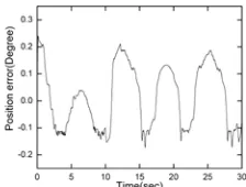
Figure 7: e1

Figure 8:α1

Figure 9:α2

Figure 10:α3

Figure 11: x1 For Classical Backstepping

(9)

[image:9.612.143.255.249.334.2]

Figure 15: e1 For Classical Backstepping

Figure 16:

α

1 For Classical Backstepping

Figure 17:

α

2 For Classical Backstepping

Figure 18: α3 For Classical Backstepping

7.

CONCLUSION

In this paper, an adaptive fuzzy backstepping is developed to control PMSM in unmeasured states. Fuzzy logic systems are used to approximate the uncertain nonlinear functions. The proposed controllers which overcome the problems of the classical backstepping guarantee that the position tracking error converges to a small scope and all the closed-loop signals are bounded. Simulation results show that the effectiveness of the proposed control method.

ACKNOWLEDGEMENTS:

The work is supported by the Jining government and the Shenyang Branch of Chinese Academy of Sciences cooperation Foundation (2010JNKJ001) and the Jining University Youth Foundation (2011QNKJ05).

REFRENCES:

[1] Harb A M, Nonlinear chaos control in a permanent magnet reluctance machine,

“Chaos, Solitons & Fractals”, Vol.19, 2004,

pp.1217-1224.

[2] Poursamad A, Markazi A H D, Adaptive fuzzy sliding-mode control for input multi-output chaotic systems, “Chaos, Solitons &

Fractals”, Vol.42, 2009, pp.3100-3109.

[3] Lin F-J, Wai R-J, Robust recurrent fuzzy neural network control for linear synchronous motor drive system, “Neurocomputing”, Vol.50, 2003, pp. 365-390.

[4] Zhou J, Wang Y, Real-time nonlinear adaptive backstepping speed control for a PM synchronous motor, “Control Engineering

Practice”, Vol.13, 2005, pp.1259-1269.

[5] Yu J, Chen B, Yu H, Position tracking control of induction motors via adaptive fuzzy backstepping, “Energy Conversion and

Management”, Vol.51, 2010, pp.2345-2352.

[6] Elmas C, Ustun O, Sayan H H, A neuro-fuzzy controller for speed control of a permanent magnet synchronous motor drive, “Expert

Systems with Applications”, Vol.34, 2008,

pp.657-664.

[7] Li Y, Tong S, Adaptive fuzzy backstepping output feedback control of nonlinear uncertain systems with unknown virtual control coefficients using MT-filters,

“Neurocomputing”, In Press, Corrected Proof.

[8] Yu J, et al, Adaptive fuzzy tracking control for the chaotic permanent magnet synchronous motor drive system via backstepping,

“Nonlinear Analysis: Real World Applications”,

(10)

[9] Chen B, Tong S, Liu X, Fuzzy approximate disturbance decoupling of MIMO nonlinear systems by backstepping approach, “Fuzzy Sets

and Systems”, Vol.158, 2007, pp.1097-1125.

[10] Qian W, Panda S K, Xu J X, Periodic speed ripples minimization in PM synchronous motors using repetitive learning variable structure control, “ISA Transactions”, Vol.42, 2003, pp.605-613.

[11] Peng Y-F, Robust intelligent backstepping tracking control for uncertain non-linear chaotic systems using H[infinity] control technique, “Chaos, Solitons & Fractals.”, Vol.41, 2009, pp. 2081-2096.

[12] Li C, Tong S, Wang W, Fuzzy adaptive high-gain-based observer backstepping control for SISO nonlinear systems, “Information