ARABIC TEXT CLUSTERING BASED ON K MEANS ALGORITHM WITH SEMANTIC WORD EMBEDDING

ISSN: 1992-8645 www.jatit.org E-ISSN: 1817-3195

3144

A METAHEURISTIC APPROACH FOR STATIC

SCHEDULING BASED ON CHEMICAL REACTION

OPTIMIZER

1_{OMAYYA MURAD,} 2_{RIAD JABRI,} 3_{BASEL A. MAHAFZAH}

1,2,3 _{Computer Science Department, The University of Jordan, Amman 11942, Jordan}

E-mail: 1_{umaiya.murad@gmailcom,} 2_{[email protected],} 3_{[email protected]}

ABSTRACT

Over the past several decades, scheduling has emerged as an area of critical research, thereby constituting a requisite process for myriad applications in real life. In this regard, many researchers have experimented and utilized various optimization algorithms to obtain optimized schedules. It is also noteworthy that the concepts of some optimization algorithms are essentially derived from nature. This paper aims to augment a compiler using a chemical reaction optimizer in order to identify an optimized instructions static schedule capable of being used within both single and multicore computer systems. This scheduling algorithm, which is denoted as SS-CRO (static scheduling using chemical reaction optimizer), is unique in that it provides alternative schedules involving different costs. Subsequently, SS-CRO tests the schedules in accordance with different types of instructions dependencies before making an appropriate selection. SS-CRO demonstrates that it can not only provide different schedule orders, but also make a competent selection of accepted solutions, whilst dismissing the inappropriate ones in a reasonable span of time. So, this paper presents SS-CRO algorithm that is used to obtain an optimized static scheduling, where SS-CRO has been implemented and evaluated analytically and experimentally. As analytical results, the number of

steps for the SS-CRO approximately is O(Num_iteration×CROFun), where CROFun is the number of steps

of the selected function. In the experiments results, SS-CRO achieved better execution time and higher accepted solutions in comparison with other optimization algorithms such as; SS-DA (static scheduling using duelist algorithm) and SS-GA (static scheduling using genetic algorithm). Furthermore, SS-CRO achieved the maximum percentage of number of solutions with respect to the execution time of all experiments for all proposed input cases, which is ranged as (10%-30%).

Keywords: Chemical Reaction Optimizer, Compiler, Instruction Set, Metaheuristic Approach, Static

Scheduling

1. INTRODUCTION

In recent times, the concept of optimized scheduling gained prominence across a plethora of applications. Within this overarching theme, the computer architecture finds inclusion among such applications wherein a number of approaches have been adopted with a view to fulfil the onerous task of enhancing the performance of computations. Notably, the trend to improve the performance of computer applications has it genesis in two distinct avenues. First, the efficacy of dynamic scheduling in augmenting the speed as well as capacity of the hardware has been recognized. Second, static scheduling is known to improve the quality of

3145

graphic processing units. While the dynamic

scheduling has been known to be used more frequently, the element of exorbitant cost has been

amatter of disappointment. It is for this reason that

static scheduling is utilized as a complementary approach to dynamic scheduling. However, the majority of existing static scheduling techniques is premised on classical dependency analysis and is characterized on the basis of its stymied capabilities. Against this backdrop, this study is aimed at meeting the need for a refreshing approach to resolve this problem. Correspondingly, chemical

reaction optimizer has demonstrated its

efficaciousness in several fields and hence, can be used to make improvements in a program’s static scheduling at different levels, including tasks and instruction. This, in turn, is justified by the following facts:

 A program denotes a set of instructions that

are executed based on their inter-dependencies. The compiler can be used to generate an optimized static schedule of these instructions [3]. Actually, the optimized schedule is intended to feed the pipeline whilst to simultaneously executing the instructions. Thus, bridging the gap in pipeline stages, as demonstrated by the authors of [5]. In pipelining, the main predicament is to maintain all the stages in their entirety with a view to reduce latency to the maximum extent possible using an intelligent compiler. According to [6], this can be accomplished by

instruction reordering/serialization, and

multiple instruction issues.

 The chemical reaction is a natural process that

causes some substances from an unstable state to become stable through a number of iterations [7]. Concurrently, this process necessitates energy preservation in accordance with the conservation of energy law whilst transferring it from one entity or form to another. As a result, it becomes possible to replicate these laws to resolve problems in different regions; authors of [8] termed this process as a nature-inspired computing. Correspondingly, the authors of [7] presented chemical reaction as a metaheuristic for optimization. The chemical reaction optimizer (from now CRO) algorithm begins with a set of input values as an input vector, Subsequently, the vector will be manipulated by four types of operations (on-wall ineffective collision; decomposition; inter-molecular ineffective collision; and synthesis)

to obtain an optimized solution whilst maintaining a set of constraints.

To reiterate, static scheduling and CRO algorithm performs operations with similar effects. Hence, a correspondence can be established between their respective operations. Therefore, we will incorporate chemical reaction optimizer as a tool for a static scheduling in the proposed algorithm static scheduling using chemical reaction optimizer (from now SS-CRO), in this paper. Notably, once we establish a correspondence between molecules and program segments the four types of chemical reactions are considered to be ways of optimization. Subject to constraints (instruction dependencies), such optimization is reduced to instruction reordering/serialization and decomposition into multiple issues (segments).

Meanwhile, three cases of a program

dependency graph (PDG) of a program segment

were proposed to test SS-CRO, which are varies in the dependencies between their nodes (i.e. program

segment instructions). The less dependency a PDG

has, the more solutions achieved by CRO. SS-CRO is been compared with two distinct optimization algorithms such as static scheduling using duelist algorithm (from now SS-DA) and static scheduling using genetic algorithm (from now SS-GA). SS-CRO achieved the lowest execution time for all proposed input cases, and for all iteration numbers. On the other hand, SS-CRO achieved the maximum percentage of accepted solutions (from now PerSol) with respect to execution time, which was ranged as (10%-30%), while PerSol of the SS-DA achieved the moderate range as (0%-21%), and the minimum values of PerSol was for the SS-GA, which was ranged as (0%-1%).

The main objectives of this paper are: define the static scheduling of instructions, formalize the program instructions dependencies, decompose the program into basic blocks and reflect the program dependencies using CRO, present and apply the Chemical Reaction Optimizer to obtain an optimized static scheduling, implement static scheduling using CRO, evaluate analytically and experimentally the SS-CRO algorithm.

ISSN: 1992-8645 www.jatit.org E-ISSN: 1817-3195

3146 The remaining portion of this paper is

organized in the following manner: Section 2

undertakes a description of literature review, while

Section 3 presents a brief background of CRO, GA

and DA. Meanwhile, section 4 demonstrates Instruction Static Scheduling and CRO. On the

other hand, Section 5 elucidates the proposed

algorithm SS-CRO pertaining to instructions static

scheduling in compilers. Section 6 outlines the

results of the experiment, whereas Section 7

summarizes the conclusions.

2. LITERATURE REVIEW

In an extensive body of extant study, researchers have proposed a number of evolutionary algorithms in order to solve complex problems. These algorithms demonstrated their ability to solve range of problems. One of the areas that evidence the usage of evolutionary algorithms is optimizing task schedules of various types of problems. Most of the researchers have looked toward nature to identify possible solutions. For example, authors of [9] came up with the particle swarm optimization (PSO), while the author of [10] and the authors of [11] put forward the memetic algorithm (MA). Similarly, differential evolution (DE) was presented by authors of [12], ant colony optimization (ACO) was the brainchild of the work in [13], harmony search (HS) was postulated by authors of [14], Sea Lion optimization algorithm presented by authors of [15].

In the past, researchers have also used evolutionary algorithms such as genetic algorithms to optimize task scheduling as well as to solve the problem of traveling salesman problem (TSP); for this purpose, authors have adopted interesting approaches to arrive at a feasible solution [16, 17]. In particular, authors of [16] used genetic algorithms to provide optimal or near optimal solutions for scheduling various tasks on several processors. This evolutionary algorithm can be helpful in augmenting the efficiency of executing programs on multiprocessor scheduling problem in parallel. They also extended their solution by assigning the problem to appropriate processors and focusing on the reduction of execution time of the entire system. In addition to creating some genes to present the tasks that can be configured in a directed graph to underpin. the inter-dependencies of tasks, author of [16] used three main operators in order to manipulate their presented algorithm, including selection, crossover, and mutation. Finally, they implemented the entire genetic

algorithm scheduling precedence on constrained task graphs.

In particular, many heuristic algorithms were employed in different fields to solve range of problems, such as; solving the travelling salesman problem [18, 19]. Meanwhile, authors presented performance evaluation for different parallel heuristic algorithms as shown in [20-22]. Moreover, many metaheuristic algorithms were proposed to solve range of problems such as; task scheduling in cloud computing using vocalization of humpback whale optimization algorithm [23]; test Jordan University Hospital Databases (JUH DBs) exceptions by applying genetic algorithm [24]; using genetic algorithm as a test data generator [25]; using multiple-population genetic algorithm for branch coverage test data generation [26]; a solution for traveling salesman problem using grey wolf optimizer algorithm [27].

Meanwhile, the authors of [28] presented a common model to schedule tasks with advance reservation requests as well as computational batch tasks. In addition, they lowered the effect of advance reservations on a schedule quality by putting forward unambiguous on-line scheduling policies and generic advices.

Correspondingly, authors of [29] formulated the (primal) problem as a nonlinear integer

programming model. In addition, they

demonstrated their ability to solve this problem by resolving a corresponding dual problem using a nonlinear relaxation. More specifically, they utilized genetic algorithm since both primal and dual problems are NP-hard. They observed that the genetic algorithm consistently outperformed a standard mathematical programming package with regard to computation time and solution quality.

Analogously, authors of [30] put forth a three-stage algorithm for resource-aware scheduling of

computational jobs within a large-scale

3147 Similarly, authors of [32] presented an algorithm named as clusters dimension exchange method (CDEM) in order to augment both the load balancing technique and job scheduling within the OTIS (Optical Transpose Interconnection System)-hypercube interconnection network.

In [33], authors leveraged the efficacy of the chemical reaction optimization algorithm for the purpose of multi-objective optimization. By premising their work on non-dominated sorting, they were able to propose a new quasi-linear with average time complexity concerning the quick non-dominated sorting algorithm. Additionally, the authors compared their findings with several multi-objective algorithms on a gamut of benchmarks problems, thus highlighting the efficiency and effectiveness of their proposed algorithm.

Meanwhile authors of [34] utilized CRO to resolve the printed circuit board drilling problem (PCBDP), which is the primary component of computers and electronic equipment (PCB). The authors focused their attention to solving the problem of controlling the drilling machine within the drill holes in PCB. More specifically, they aligned it as a TSP. Finally, they used CRO to solve the problem, which was subsequently implemented as an illustration of TSP.

In [1], authors presented a twofold generic parser that simulated the behavior of multiple parsing automata. This proposed parser, which was an extended version of Position Parsing Automation (PPA), accepted the strings drawn from regular tree grammar, context-free grammar, or both of them. Importantly, this parsing enhancement can help compilers perform their jobs efficiently.

Correspondingly, authors of [35] presented a hybrid load balancing algorithm that chained cubic tree interconnection network. This algorithm combines two common load balancing strategies: dynamic load balancing and parallel scheduling. In the study, the performance was measured using several metrics. In addition, the presented algorithm underpinned the importance of parallel scheduling with dynamic load balancing.

Meanwhile, authors of [36] presented a system that identifies transformation algorithms for an input program where programs’ specific features is been considered.

Finally, authors of [2] proposed the implementation of a predictive bottom-up parser in

two versions. Both versions were used as components of the proposed algorithm that simulates the operation of a shift–reduce automaton, which is defined and constructed by integrating its parsing actions with conflict resolution, reduction prediction, and error recovery.

3. BACKGROUND

This section introduces a brief background of three optimization algorithms; namely, chemical reaction optimizer (CRO), genetic algorithm (GA) and duelist algorithm (DA).

First, the chemical reaction optimizer that is presented by authors of [7], and it is inspired from the chemical reaction between unstable molecules. The molecular go through four different reactions defined by the authors of [7], which are on-wall

ineffective collision; decomposition;

inter-molecular ineffective collision; and synthesis. Subsequently, the unstable molecules are converted to stable one. Importantly, this algorithm extracted it's constrains from the low energy that is used in the natural chemical reaction, which is based on energy preservation where this energy should be reserved before and after any reaction. Actually, authors used CRO to solve several problems, and the results achieved by CRO were competitive. For more details in regards of CRO can be found in [37-40].

Second, genetic algorithm (GA) is a well-known metaheuristic algorithm presented by authors of [41]. Basically, GA is been inspired from the natural selection and used for solving

constrained and unconstrained optimization

ISSN: 1992-8645 www.jatit.org E-ISSN: 1817-3195

3148 Third, duelist algorithm (DA) is a recent optimization algorithm, which inspired by how the duelist improve their skills in a duel [44], which is considered as a pure random algorithm. Actually, DA is based on human fight and how they improve their capabilities from each duelist, where it starts with a duelist population and chooses randomly two duelists to fight. Thus, in every duel there is a winner and a loser, where a loser learns from the winner. On the other hand, the winner uses new skills to improve its fighting capabilities, where the duelist with highest capabilities will be noted as

champions. Subsequently, champions are

responsible to train new duelists and duelists with worst capabilities will be eliminated. Thus, for more details in regards of DA can be found in [44-46]

4. INSTRUCTIONS STATIC SCHEDULING AND

CRO

In static scheduling, the compiler can potentially reorder the program instructions in varying orders to reduce the latency whilst concurrently saving the inter-dependencies between the instructions. Notably, these interdependencies imply that the program yields the same results, at a reduced cost (CPU time) [5]. Furthermore, it is possible to perform static scheduling by decomposing program segment into multiple ones,

with a proper serialization to maintain

interdependencies between instructions. The multiple segments constitute code parallelization. Such segments are appropriate for multicore and multiple issue processors.

On the other hand, the primary objective of CRO is to present an optimized solution for a problem. This process is underscored by the contours of different types of chemical reactions

such as: on-wall ineffective collision,

decomposition, inter-molecular ineffective

collision, and synthesis

[

7

]

the static scheduling in terms of

reordering/serialization and generation of multiple schedules.

The static scheduling and its reflection by CRO are formalized as follows:

Let <I1,…, In> be a sequence of instructions

constituting a program P.

Let C = {ci,…, ci} be a set estimated execution

costs of the individual instructions.

Let D= {D12,…, Dij} be a set of instruction

dependencies as described in Section 3.1. Dij

represents the dependency between Ii and Ij.

Let a program dependency graph (PDG) be

defined as PDG = (N, E, C), where:

 N= {np1, np2, np3,…,npn}is a set of nodes

such that npi represents Ii . In [47], authors

pretended that there are two distinct kinds of

nodes in a PDG such as:

o Regular node that has a regular

statement such as; assignment statement

o Control node that has a control

statement such as; a condition in a loop or an if statement.

 E = {e11, e12 ,e3 ,…,eij }is a set of edges such

that eij represents Dij between the nodes npi

and npj and labeled by the cost cj. In [47],

authors pretended that there are two distinct

kinds of edges in a PDG such as:

o Solid edge that presents data a

dependency or a name

dependency

o Dashed edge that represents a

control dependency

Let an optimized static schedule S respective to

P be defined as PDG decomposition maintaining

the constraints implied by D. Such decomposition

constitutes specific order O(PDG) of the PDG

nodes. It is obtained through iterative application of the following operations:

 Reordering/Serialization operation SRO

(PDG)S=O<np1, np2, np3,…,npn> is a

sequence of nodes in a specific order with

minimal cost and satisfying D.

 Multiple scheduling operation MS(PDG) S,

where S=S1, …, Sn is a decomposition of PDG

into multiple schedules S1= O<np1,np2,

np3,…,npm>,…, Sn=O< npl+1, npl+2 , npl+3 …,

npn> with minimal cost and satisfying D.

The reflection of static Scheduling is achieved by establishing a correspondence between its four

reactions and the operations SRO

(reordering/serialization) and MS (multiple

scheduling). Reflected static scheduling is then

defined by the composite function

FCRO(PDG)=OCDCICSN(PDG)S, where OC,

DC, IC and SN are correspondent functions to the CRO reactions: on wall ineffective collision;

decomposition, inter-molecular ineffective

3149 implementation of FCRO is given in Section 5. In subsequent section we use words instruction and node interchangeably. This is justified by the definition of PDG.

4.1 Dependencies in Instructions Static

Scheduling

This section includes the definition of the primary types of dependencies, as defined by authors of [5]. Instructions static scheduling comprises of three types of dependencies: data dependency, name dependency, and control dependency. Dependencies manifest in a schedule between two instructions Ii and Ij under specific conditions, as enlisted below for each type of dependencies. Once we define the sets

D={D12,…,Dij}and CONT={ContIi,…,ContIm}

respective to data (name) and control dependencies

a PDG respective to an input program P can be

constructed as given by the formal definition. In addition, they will be used as the objective function (from now OF) in the SS-CRO, which will be used further to evaluate the effectiveness and the acceptability of the solution. The construction of D and CONT proceeds as given below.

Let P=<I1, …,In> denotes a sequential schedule

of n instructions of a programsegment P we define:

 PRO(Ii) as the set of data operands

that hold the results from Ii, and

 USE(Ii) as the set of data operands

used in the instruction Ii. Let us assume that USE(Ii), and PRO(Ii), ≠

∅, ∀i. Subsequently, an edge eij between npi and npj in PDG will be exists if and only if there is any kind

of dependencies such as dij∈D or

ContIi ∈ CONT. In addition, the cost of eij is defined as cij, where cij∈C.

In congruence with the observation by authors of [5], we will define the instruction dependencies set D= {D12,…,Dij}in terms of

 Dij= USE(Ii) ∈PRO(Ii)       

(1)

 Dij=USE(Ik)∈PRO(Ii) ≠ ∅, and

USE(Ij)∈PRO(Ik )≠ ∅,∃Ik (2)

Where dependencies defined in Equation 1 and 2 are used to represent data dependency (also referred

to as true data dependency), wherein, Ij signifies the

data dependent on Ii if any of the following

conditions holds:



instruction Ii, as illustrated in Equation 1, i.e. in the PDG there is an edge eij between npi and npj.



instruction Ik, while Ik data is dependent on

instruction Ii, as depicted in Equation 2, i.e. in the PDG there are two edges eik between npi

and npk and ekj between npk and npj.

 Dij= ri∈PRO(Ii) and

ri∈USE(Ij),where ∃ri (3)

 Dij=(ri∈PRO(Ii)∩USE(Ii ))and ri∈ (USE(Ij)∩PRO(Ij)),where ∃ri   (4) 

Meanwhile, dependencies defined in Equation 3 and 4 are used to represent name dependency occurs in case there is an absence of data flow between two instructions, but they make use of the same registers or memory locations. Authors of [5] presented the following two types of name dependency:

 An anti-dependence between instruction Ii and

Ij takes place when Ii writes an operand ri that

is read by Ij. Therefore, the original order needs to be preserved in order to ensure that every instruction involves the correct value, as

illustrated in Equation 3, i.e. in the PDG there

is an edge eij between npi and npj.

 An output dependence occurs when two

instructions Ii and Ij are writing on the same

operand ri, which is why we should maintain

the order of the instructions in order to make sure that the last value is written within the register, as evidenced in Equation 4, i.e. in the PDG there is an edge eij between npi and npj.

Control dependency takes place when an instruction execution gets controlled by such a

branch. We define the set CONT as follows. Let us

assume that Ii in a program P features a control instruction and subsequently dominant to the sequence of dependent instructions<Ij+1,Ij+2,

…..,Im>. Then we define a control dependency

CONT such that ContIi = <ConIj+1, …,ConIm> ∈

CONT in schedule S. Assume ∀Ii ∈S, ∃!O(Ii) where

O(Ii)is the order of Ii in P (where Ii refers to an

ISSN: 1992-8645 www.jatit.org E-ISSN: 1817-3195

3150 control dashed edge that controls the order of the instruction according to the control node which reflects a condition statement in the loop/if statement. Analogously, the two constraints pertaining to control dependency are as follows:

 An instruction controlled by a branch cannot

move before, which will prevent the branch from controlling it, as illustrated in Equation

5. In a PDG, a control node should be

connected with all of its successors by dashed edge.

ContIi=O(Iik )>O(Ii),∀Iik∈ContIi (5)

 An instruction out of the branch cannot be

made after the branch, which, in turn, will control its execution, as depicted in Equation

6. In a PDG, a dependent node should be

connected with its predecessors by a dashed edge.

ContIi=O(Iik )>O(Iim+1),∀Iik∈ContIi (6)

4.2 Definitions and Examples of Instructions

Static Scheduling Using CRO Reactions

This section defines chemical reaction in accordance with the instructions of the static scheduling problem. Four distinct reactions are observed in the iterations made in CRO: (i) on wall ineffective collision (OC); (ii) decomposition (DC); (iii) inter-molecular ineffective collision (IC); and (iv) synthesis (SN). Each of these reactions has its own properties, such as the number of actual inputs and the number of outputs needed. The following subsections depict an example for each type of

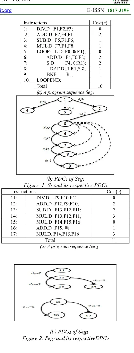
reaction using two program sub-segments Seg1 and

Seg2. These sub-segments and their respective

PDGs, are shown in Figure 1 and Figure 2,

respectively. Notice that both sub-segments are

extracted from the same program segment P, for

illustrative purpose. One more, instruction number

10 is excluded from the PDG because its job is

been demonstrated in the PDG implicitly

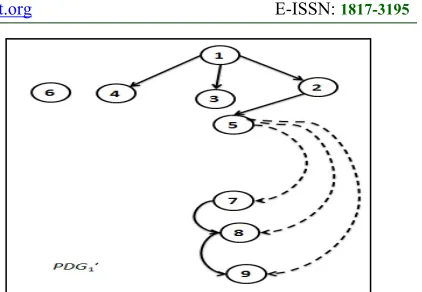
Instructions Cost(c)

11: DIV.D F9,F10,F11; 0 12: ADD.D F12,F9,F10; 2 13: SUB.D F13,F12,F11; 2 14: MUL.D F13,F12,F11; 3 15: MUL.D F14,F15,F16 0

16: ADD.D F15, #8 1

17: MULD. F14,F15,F16 3

Total 11

(a) A program sequence Seg2

(b) PDG2 of Seg2

Figure 2: Seg2 and its respectiveDPG2

4.2.1 On wall ineffective collision

According to our purpose, we interpret the on

wall ineffective collision (OC) as a molecular S

(old schedule) hits an outer object. Subsequently, a reordering of the instructions will be resulted. The reflection of static scheduling by OC will be reduced to altering the order of the instructions in

Instructions Cost(c) 1: DIV.D F1,F2,F3; 0 2: ADD.D F2,F4,F1; 2 3: SUB.D F5,F1,F6; 1 4: MUL.D F7,F1,F8; 1 5: LOOP: L.D F0, 0(R1); 0 6: ADD.D F4,F0,F2; 2 7: S.D F4, 0(R1); 2 8: DADDUI R1,#-8; 1 9: BNE R1, 1 10: LOOPEND;

Total 10

(a) A program sequence Seg1

(b) PDG1 of Seg1

3151

schedule S and providing a new schedule S’ (new

molecular). Where S’ has a new PDG’ that has the

same nodes of PDG, but reordered. Formally, we

define OC as a reordering operation SRO over a given flow-graph, as given by Equation 7.

OC = SRO(PDG) → PDG′: S → S′

(7)

Where S refers to a schedule of n instructions S = O<I1,…,In>, such that each Ii has a specific order,

and the initial PDG of S has the dependency set D

and estimated cost c. The on wall ineffective

collision is then defined as a reordering process to produce S′=O<I1, …,In>, where ∃Ik ∈S and ∃Ik ∈S′

are two distinct instructions have the same order k

in both schedules S and S′, but they are not equal to

each other. Moreover, S′ preserves the data

dependency exists in S. On the other hand, PDG′is

the flow-graph of S′after applying OC on S. PDG′

has the same nodes of PDG, but in a different

order, where PDG′ preserves data dependency set D

of S. On the other hand, the estimated cost of PDG′

is c′, where c′≤ c.

Finally, if c′ >c or D is not preserved then

PDG′ will be dismissed. This, in turn, necessitates

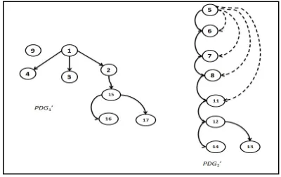
its exclusion from the solution area. To illustrate, the reaction moves one instruction like instruction 6

(node np6) from the LOOP command and extricates

it from the LOOP boundaries (it may be noted that LOOP and BNE are used to signify the beginning and ending boundaries of the instructions inside the loop statement). Hence, if any instruction is moved out of these boundaries, the solution needs to be summarily dismissed, as illustrated in Figure 3,

wherein OC function has been applied on S1. In this

example, in the PDG′ a dashed edge is been broken

as a result a control node np5 lost one of its’ successors, which it is np6 and np6 lost its’ control predecessor np5. i.e. PDG′ does not preserve the

dependency set D, so it will be dismissed.

This can be accomplished by ascertaining the inter-dependencies between instructions in the schedule prior to and after the reaction, that is, the

total new energy resulted by PDG’ such as the sum

of PE’ and KE’ should be less than or equal to the

total energy of the original PDG such as the sum of

PE and KE, as depicted in Equation 8.

PE’ + KE’ ≤ PE + KE (8)

Figure 3: PDG1 after on wall ineffective collision

4.2.2 Decomposition

In this paper, the decomposition (DC) occurs

when a molecular S (old schedule) collides with the

wall and yields two new molecules such as S′1and S′2.The reflection of static scheduling by DC is shown as the old schedule will be divided to create new schedules. In the realm of static scheduling, this can be considered as a multiple issue scheduling, where a program segment can be split into multiple pieces (sub-program segments) before being distributed across more than one processor. Formally, we define DC as a multiple scheduling process MS of a given flow-graph, as given by Equation 9.

DC= MS(PDG) → (PDG′1, PDG′2):

S→(S′1,S′2) (8)

Notably, S denotes a schedule of n instructions S = O<I1, …,In> that has an initial flow-graph such

as PDG. Importantly, the decomposition reaction

signifies a multiple issue scheduling process carried out by dividing S into two sub-schedules such as S′1

of k instructions S′1 =O<I1, …,Ik> as well as S′2 of

m instructions S′2 = O<I1, …,Im>, where m+k = n

and S′1 and S′2 preserve the data dependencies

existing in S. Moreover, PDG’1 and PDG’2 are the

flow-graphs of S′1 and S′2 respectively. PDG’1 and

PDG’2should preserve the data dependency set of

PDG, unless they will be dismissed.

In the case of instructions static scheduling, we will compute the total energy for the new schedules and ascertain whether the dependencies between the instructions and the total energy have been reserved, as shown in Equation 10. If that is not the case, we will not only obtain a higher cost, but also risk computing wrong schedules. Therefore, we will dismiss the new incorrect schedules from the solution set, indicating that we will lose some data

ISSN: 1992-8645 www.jatit.org E-ISSN: 1817-3195

3152 Consequently, energy conservation is not satisfied in this analysis, which builds the case for excluding the new particles. This will manifest in the division and be determined based on whether it occurs in the middle of a loop instruction or separates two dependent instructions.

PE’1 + KE’1+ PE’2 + KE’2≤ PES + KES

(9)

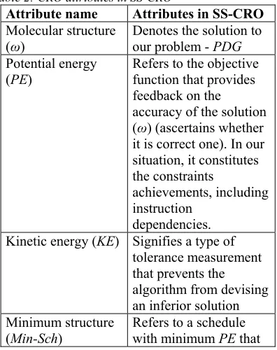
An example of an unacceptable decomposition becomes apparent when new schedules are shown to hold the dependent components presented by two or more instructions and the reaction split them, as illustrated in Figure 4, where it becomes evident that decomposition reaction is been applied on S1.

In this example, the new flow graphs PDG’1 and

PDG’2did not preserve the dependency D of PDG1,

where node np5 lost its dependent edge from node

np2, so the new flow-graphs will be dismissed.

Figure 4: PDG1 after decomposition

4.2.3 Inter-molecular ineffective collision

According to our approach, the inter-molecular ineffective collision (IC) occurs when two distinct schedules hit each other, resulting in two new schedules. In this instance, the reflection of static scheduling by IC on S1 and S2 will interchange the

instructions between them to provide two new schedules S′1 and S′2. This reaction is unique in that

it will definitely find acceptance if the new schedules save dependency sets and do not cost more than their predecessors. Formally, we define IC as two successive operations of multiple scheduling MS and reordering SRO of given two flow-graphs, as illustrated in Equation 11. On the other hand, the data dependency and total energy should be saved after this reaction, as shown in Equation 12.

IC = MS(SRO(PDG1,PDG2))→

(PDG′1,PDG′2): (S1,S2) →( S′1,S′2) (10)

PE’1 + KE’1+ PE’2 + KE’2≤ PE1 + KE1+ PE2 + KE2 (11)

Clearly, S1 signifies a schedule of k instructions

S1=O<I1, …,Ik> and S2 refers to a schedule of m

instructions S2 = O<I1, …,Im>, where m+k = n. The

respective flow-graphs of S1 and S2 are PDG1 and

PDG2, respectively. The reflection of static

scheduling by IC is essentially a combination of reordering SRO and multiple scheduling MS operations by combining both schedules, reordering them, and finally re-dividing them into two new schedules S′1 of g instructions S′1 = O<I1, …,Ig> in

addition to S′2 of h instructions S′2=O<I1, …,Ih>,

where g+h=n, and S′1 and S′2 will save the data dependences existing in S1 and S2.

In this reaction, a scenario may arise wherein two independent schedules impart two new independent schedules after they hit each other (before the reaction). Consequently, such a solution should be aborted if the execution costs would be higher or data dependency set is not saved, as illustrated in Figure 5, where IC has been applied on S1 and S2. In this reaction, both operations SRO

and MS will be used to get PDG’1and PDG’2, those

have same nodes of PDG1and PDG2, and preserve

dependency. In this Example, the dependency

between np2 and np5 was lost, while two new wrong

dependencies were been added between np2 and

np15, and between np8 and np11. Also one wrong

control dependency has been added between np5

and np11, i.e. a foreign instruction entered the loop

statement. This implies that PDG’1and PDG’2

should be dismissed.

Figure 5: PDG1 and PDG2 after IC

4.2.4 Synthesis

Synthesis (SN) reaction is the opposite of decomposition reaction and refers to a scenario where two schedules S1 and S2 hit each other to

yield a single schedule S’. In this instance,

3153 issue in static scheduling. This solution can be deemed safe if it does contribute towards energy conservation, as shown above and illustrated in

Equation 14. Formally, we define SN as a

reordering SRO process of given two flow-graphs, as shown above as illustrated in Equation 13.

SN=SRO(PDG1,PDG2) → PDG′:

(S1,S2) →( S′) (12)

PE’ + KE’ ≤ PE1 + KE1+ PE2 + KE2 (13)

Clearly, S1 denotes a schedule of m instructions

S1 = O<I1, …,Im> and S2 be a schedule of k

instructions S2 = O<I1, …,Ik>. Synthesis reaction is

a reordering process that combines both schedules S1 and S2 into a single schedule S′, such as S′= <I1,

…,In>, where n= m+k and S′ preserves the data

dependences existing in S1 and S2.

Figure 6 illustrates an example of rejected solution resulted by synthesis between two independent schedules and affect each other’s results when they hit each other. Therefore, it is necessary to ignore this particular solution. The result of SRO operation over PDG1 and PDG2 in

this example is a new flow graph PDG’. In PDG’, a

new wrong control edge is been added between np5

and np11, which violates the existing dependency

set, and so PDG’ should be dismissed.

Figure 6: PDG1 and PDG2 after Synthesis

4.3 CRO Meanings and Attributes in SS-CRO

Given a PDG respective to program P, the

implementation of static scheduling for P by CRO

is reduced to applying the composite function

FCRO(PDG), as depicted by Figure 7. FCRO is

implemented by the proposed algorithm SS-CRO as illustrated in Algorithm 1, which is been inspired from the CRO algorithm that posited by the authors

of [7]. SS-CRO has a PDG of a program segment

as its input. PDG is then manipulated by the four different functions respective to CRO reactions as depicted in Section 5.2, which will yield a distinct set (solution set) of candidate solutions. Subsequently, this algorithm will ascertain all types

of dependencies D to verify whether the solution is

correct or if it needs to be dismissed.

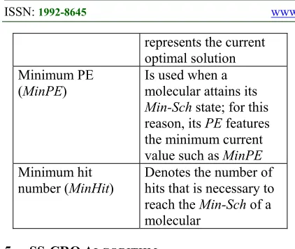
Table 1: Chemical meaning as used in SS-CRO algorithm

Chemical Meaning SS-CRO

Molecular structure Candidate solution

– PDG

Potential energy Value of

dependency

preserved of a PDG

for such candidate

solution (which

preserved all kinds of dependencies)

Kinetic energy Measure of

tolerance of having

worse PDG

Minimum structure Current optimal

PDG

Based on CRO algorithm presented by the author of [7], Table 1 enlists the meanings of chemical reactions that will be used within the SS-CRO algorithm, and Table 2 enlists the interpretation of CRO attributes in SS-CRO. Finally, the execution time complexity analysis will be explained in section 5.3.

Table 2: CRO attributes in SS-CRO

Attribute name Attributes in SS-CRO

Molecular structure

(ω) Denotes the solution to our problem - PDG

Potential energy (PE)

Refers to the objective function that provides feedback on the accuracy of the solution (ω) (ascertains whether it is correct one). In our situation, it constitutes the constraints

achievements, including instruction

dependencies.

Kinetic energy (KE) Signifies a type of

tolerance measurement that prevents the algorithm from devising an inferior solution Minimum structure

ISSN: 1992-8645 www.jatit.org E-ISSN: 1817-3195

3154 represents the current

optimal solution Minimum PE

(MinPE) Is used when a molecular attains its Min-Sch state; for this reason, its PE features the minimum current

value such as MinPE

Minimum hit

number (MinHit) Denotes the number of hits that is necessary to reach the Min-Sch of a molecular

5. SS-CROALGORITHM

In this subsection, the implementation of SS-CRO will be presented. As shown in Algorithm 1, SS-CRO algorithm has three phases that operates in the following order: initialization phase; iteration phase; and solution confirmation phase. The workflow of the algorithm is shown in Figure 7. The following paragraphs will explain the SS-CRO algorithm phases in details.

In the initialization phase, the algorithm generates threshold values of some variables, which

includes PDG_size that equals the number of nodes

of the initial DPG, the number of iterations required

in the iteration phase. Initially, Min-Sch is assigned

to be the initial PDG that (PDG1) as the best

solution,and the solution set holds only PDG1. The

first seven lines in the algorithm make the entire process evident. In particular, the step of calling the objective function OF will ascertain the dependency for each node and its’ corresponding

edge in its’ PDG (see Section 4.1), before returning

the nodes dependency state and its PE and KE

values. Thus, MinPE will get its initial value as the

PE of PDG1, and the MinHit equals to zero.

Furthermore, the algorithm checks if the initial

PDG1 has less than two nodes it will be terminated,

because it will be unable to apply any of its functions.

In the iteration phase, the algorithm

commences with the consideration of the PDG1as

the most optimal solution, as shown in SS-CRO algorithm. Thereafter, this algorithm will select the

type of requisite collision by verifying molecule

(the available number of PDG in the solution set).

The algorithm forces PDG to be decomposed by

calling DC, when the molecule equals one and the

existing PDG is dividable. Subsequently, the

algorithm applies the SRO operations on one

particular PDG such as; calling OC or DC

functions. Since it will only feature one PDG in the

first instance with at least two nodes. Thus, the algorithm selects the DC function in the event the splitting option can be implemented. Importantly,

this new solution will ensconce two valid PDG’1

and PDG’2 that will be checked and evaluated to

determine their accept ability. Alternatively, the OC function will be chosen if the splitting cannot be

accomplished, which may give one valid PDG’.

Clearly, the entry of any PDG’ resulted from either

OC or DC will be added into the solution set that is predicted to be in the selection made by the algorithm in next iterations. Once, the proposed

algorithm has two valid PDG in the solution set it

will be possible to apply both kinds of operations: the SRO; and the MS operations. As an implication, the algorithm makes a random selection between SRO and MS operations. With regard to the SRO operations, it undertakes an evaluation to determine

whether the PDG’j can be reordered or divided into

more than one PDG. With regard to the MS

operations - the process of selecting the reaction is predicated on the ability to merge the two available

graphs such as PDG’j and PDG’h. Correspondingly,

the algorithm will select SN function if the merging ability is found to exist. However, if that is not the case, the algorithm will select the IC function.

Further iterations are performed to obtain an optimal solution. However, the iteration phase will commence if the number of iterations are ended or it is unable to identify a better solution.

In the solution confirmation phase, the

algorithm evaluates the identified PDG in order to

project the ideal PDG on the basis of the functions

carried out in each run to finalize the SS-CRO.

Figure 7: Workflow of the SS-CRO

PDG

PDG’

FCRO (OCDCICSN

(PDG))

{PDG’1 ,...,

3155 Algorithm 1. SS-CRO Algorithm (Main)

Input:PDGint

Output: {PDGint}/{PDG′1} / {PDG’1,… , PDG’n},

MinPE, MinHit

/* initialization phase */

1: int Max_sch

2: Global Solution_set ={PDGint}

3: Global Min_Struct = PDGint, MinPE = PE,

MinHit = 0

4: Max_sch = PDG_size(PDG1)/2

/* PDG_size is the number of node in a PDG

Max_sch is used to be sure that a PDG is

dividable or not, but each PDG in the Solution_set has at least two nodes*/

{Min_Struct, PE, KE}= OF(PDG1)

5: Generate molecule = 1 6: If (PDG_size(PDG1)< 2)

exit;

/* Iteration phase */

7: for (int i=0;(i < Num_iteration) && (PDG_size(PDGi)> 1))

8: Generate b ∈ [0, Max_sch]

9: If (molecule == 1) || (molecule <= b) then

{

10: Randomly select PDGjfrom Solution_set /* SRO operation */

11: If PDG_size(PDGj) ≥ 2 then 12: if (divide (PDGj)) then

/* PDGj can be divided */

13: Solution_set = DC(PDGj, PE, KE) 14: else

15: Solution_set = OC(PDGj, PE, KE) 16: end if

} 17: else

{

18: Randomly select PDGj and PDGhfrom Solution_set

/* MS operation*/

19: if (merge (PDG1 and PDG2)) then 20: Solution_set = SN(PDGj, PEj, KEj, PDGh,

PEh, KEh) 21: else

22: Solution_set = IC(PDGj, PEj, KEj, PDGh,

PEh, KEh) 23: end if 24: end if

/* Solution confirmation phase */ 25: Check for any new solution

26: end for-loop

/* Final phase */

27: return Solution_set Min_Struct, MinPE, MinHit

5.1 Functions of SS-CRO

In this subsection we present Functions 1-5 that are used in SS-CRO algorithm. As shown in

Function 1, the OC function receives the PDG as an

input and makes an attempt to reorder its’ nodes. When the new order is ready, the function sends it to OF in order to validate the new order of these nodes. Additionally, if the total energy of the new order is found to be smaller than its older counterpart, the latter is obliterated and the former

is returned to the solution set. Otherwise, the PDG’

created by the function gets destroyed and consequently, status quo is maintained.

Function 1. OC() // On wall ineffective collision function

Input: PDG, PE, KE

Output: Solution_set

1: PDG'j =generate new PDG randomly 2: Call Objective function for the PDG’j 3: {Min_struct, var PE’j, KE’j} =

OF(PDG'j)

/*confirm the PDG’j or dismiss it*/

4: If (PE'j+KE’j≤ PE +KE) then

{

5: Solution_set = Solution_set – {PDG} 6: Solution_set = Solution_set ∪

{PDG'j} }

7: else

8: dismiss PDG'j

9: end if

In Function 2, the IC function depicts the

reaction between two varying graphs such as PDGj

and PDGh. Thus, IC function will merge PDGj and

PDGh and randomly split them into PDG’j and

PDG’h. Subsequently, IC function will go through

each of PDG’j and PDG’h and try to reorder their

nodes and test if they are valid PDG or not. Upon

receiving PDG’j, it reorders its nodes, and

subsequently calculates its PE′j and KE′j through

the use of OF. Upon receiving PDG’h, the same

process gets repeated for PDG’h that IC reorders its

nodes and calculates its PE′h and KE′h through the use of OF. Subsequently, the function gets the total sum of the resultant values PE′j, PE′h, KE′j and KE′h and compare it with the total sum of PEj, PEh, KEj

and KEh, if the new sum has smaller value then

PDG’j and PDG’h will be confirmed; otherwise,

ISSN: 1992-8645 www.jatit.org E-ISSN: 1817-3195

3156 function either adds two new flow-graphs to the solution set and removes the original ones, or retains the original ones in the event that the splitting and the reordering do not preserve the energy for both original flow-graphs.

Function 2. IC() // Inter-molecular ineffective collision function

Input: PDGj, PDGh, PEj, PEh, KEj, KEh// two molecules

Output: Solution_set

1: Merge both PDGj, PDGh then spilt them

randomly into PDG'j, PDG'h

2: PDG'j= randomly reorder PDG'j 3: {Min_struct, PE’j, KE’j } = OF(PDG'j) 4: PDG'h= randomly reorder PDG'h 5: {Min_struct, PE’h, KE’h} = OF(PDG'h)

6: If (PE'j+PE'h+KE'j+KE'h ≤

PEj+PEh+KEj+KEh) then /*new solutions confirmed*/

{

7: Solution_Set = Solution_Set – {PDGj,

PDGh}

8: Solution_Set = Solution_set ∪{PDG'j,

PDG'h}

}

9: else

10: dismiss PDG'j,PDG'h

11: end if

In Function 3, the DC function receives one

PDGj and divides it into two sub-graphs such as

PDG’j and PDG’h. At the beginning, DC checks the

ability of decomposing the PDGj, where if a PDGj

has less than two nodes the decomposition process

will be rejected. Subsequently, if a PDGj has more

than two nodes DC will randomly split the PDGj

into two new sub-graphs. Then it dispatches the

new sub-graphs PDG’j and PDG’h to the objective

function to obtain their PE′j, PE′h, KEj and KE′h

values, respectively. If the total sum of the resultant values PE′j, PE′h, KEj and KE′h is found to be

smaller than the original total energy, the used

portions of the original PDG gets accepted and a

PDG′j and PDG′h will be added to the solution set,

and the original one will be removed from the solution set, as illustrated in lines 4 up to11.

Moreover, the molecule will be incremented by

one, i.e. the available number of PDG in the

solution set is increased by one. Briefly, this reaction takes a PDG and then divides it into two sub-graphs (PDG’j and PDG’h) with smaller total

energy value.

Function 3. DC() // Decomposition Function Input: PDGj, PEj, KEj

Output: Solution_set

: IfPDG_size >2

2: Randomly split PDG into PDG’j,

PDG’h

3: else

return Decomposition fail

4: {Min_struct, PE’j, KE’j } = OF(PDG'j) 5: {Min_struct, PE’h, KE’h} = OF(PDG'h)

6: If (PE’j+PE’h + KE’j+ KE’h ≤PEj +

KEj) then // PDG’j and PDG’h

confirmed {

7: Solution_set = Solution_Set – {PDGj}

8: Molecule ++

9: Solution_set = Solution_set ∪

{PDG’j, PDG’h}

}

10: else

11: destroy PDG’j, PDG’h

12: end if

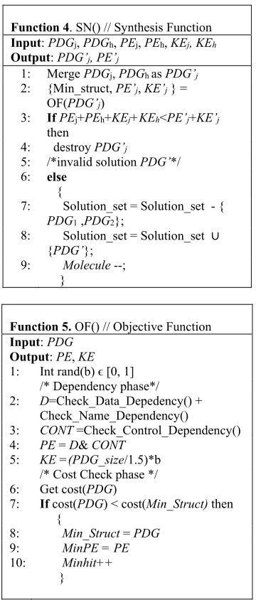
As shown in Function 4, the SN function is a very easy reaction. In particular, it takes two

distinct graphs such as PDGj and PDGh and merges

them in a new graph; such as PDG’j. Thus, SN calls

the objective function for PDG’j to get its

respective PE’j and KE’j. Subsequently, if the

resultant total energy of PE’j and KE′j is smaller than the total of original energy PEj, PEh, KEj and

KEh, then SN adds PDG’j to solution set and

removes original ones; otherwise, the merger will not occur. Moreover, the molecule will be decremented by one, i.e. the number of available

PDG in the solution list is decreased by one.

As shown in Function 5, the objective function OF is the most important function used in the algorithm. This function has two phases the dependency check phase and the cost evaluation phase. In the dependency check phase, OF receives

the PDG and evaluates all types of dependencies,

including data dependency, name dependency, and control dependency. Subsequently, it assigns a

value to the dependency status of the PDG such as

PE and computes the KE. The node or the edge

violation of any given dependency concept returns

3157 dismissed. In the cost check phase, OF calculates

the cost of the PDG and compare it with the current

best solution (Min-Sch) which has the current

lowest cost. Therefore, if PDG has a lower cost

than the current best solution, then Min-Sch will be

replaced by the current PDG; otherwise Min-Sch

will not be changed.

Function 4. SN() // Synthesis Function Input: PDGj, PDGh, PEj, PEh, KEj, KEh Output: PDG’j, PE’j

1: Merge PDGj, PDGh as PDG’j 2: {Min_struct, PE’j, KE’j } =

OF(PDG’j)

3: IfPEj+PEh+KEj+KEh<PE’j+KE’j then

4: destroy PDG’j

5: /*invalid solution PDG’*/

6: else

{

7: Solution_set = Solution_set - {

PDG1 ,PDG2};

8: Solution_set = Solution_set ∪

{PDG’};

9: Molecule --;

}

Function 5. OF() // Objective Function Input: PDG

Output: PE, KE 1: Int rand(b) ϵ [0, 1]

/* Dependency phase*/ 2: D=Check_Data_Depedency() +

Check_Name_Dependency()

3: CONT =Check_Control_Dependency()

4: PE = D& CONT

5: KE =(PDG_size/1.5)*b

/* Cost Check phase */ 6: Get cost(PDG)

7: If cost(PDG) < cost(Min_Struct) then {

8: Min_Struct = PDG

9: MinPE = PE

10: Minhit++

}

5.2 Time Complexity of SS-CRO Algorithm

In this section, we present the number of steps for SS-CRO algorithm, which depends mainly on

the number of iterations (see Num_iteration in line

7 of the SS-CRO algorithm), and the random selection of the four functions. The number of steps

for the SS-CRO approximately is

O(Num_iteration×CROFun), where CROFun is the

number of steps of the selected function. Table 3 entails the number of steps for each function, where c is a constant number, nd is the number of nodes

and ed is the number of edges. The execution time

complexity for any of the four functions

approximately is O(ed). On the other hand, the

worst case of the execution time complexity of SS-CRO is when it has a solution in every iteration and at each iteration it should check-out all kinds of dependencies that each edge node should be

checked, which leads to O(Num_iteration×ed×nd).

Table 3: Number of steps for SS-CRO and its functions Function name Number of steps

OC c+ nd+ed+1

IC 2c+ nd+ed+1

DC c+ nd+ed+1

SN c+ nd+ed+1

OF nd+ed

SS-CRO (Num_iteration)×(2c+ed+nd+1)

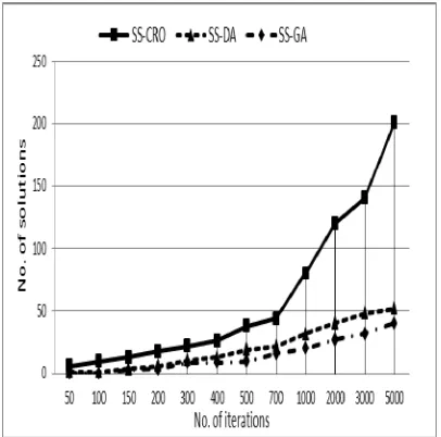
6. EXPERIMENTAL RESULTS

This section presents the experimental results of the proposed algorithm. The experiments will be done using the following three distinct cases of the

PDG of the program segment P, see section 4.2.

 First case: each node in a PDG implements an

instruction from the program segment.

 Second case: in the PDG, each control

statement such as the loop and the if statements will be clustered into one unbreakable node, and the rest will be the same as the first case.

 Third case: each group of dependent

instructions will be clustered together into one independent unbreakable node.

These three cases will be entered to the three distinct algorithms SS-CRO algorithm, SS-GA (static scheduling using genetic algorithm) algorithm and SS-DA algorithm (static scheduling using duelist algorithm). Finally, the results will be shown and compared.

In the first case, program segment P illustrates

the initial state wherein it is the input program

segment that holds both segments in Seg1 and Seg2

and their PDG’s with their associated costs, see

Figure1 and Figure 2. Program segment P will be

entered into the main algorithm SS-CRO in order to identify distinct valid schedules. In SS-CRO, when

the input PDG is presented as one molecular then it

ISSN: 1992-8645 www.jatit.org E-ISSN: 1817-3195

3158 such as PDG′1 and PDG′2 to enter the synthesis

(SN) and the intermolecular functions (IC).

For example, Figure 8 reveals a result of a valid solution found, where the first case is used. The result shows the multiple schedule of the

program segment P. The new multiple schedules

have three new schedules P′1, P′2 and P′3 with total

cost as 4, 7 and 10, respectively. Every schedule has a specific cost. The minimum cost reached for the

multiple schedules is 4 for P′1, while the maximum

cost was 7 for P′3. This can lead us that SS-CRO

can divide a program segment into optimized independent counter parts.

P′1

Instructions Cost(d)

15: MUL.D F14,F15,F16 0

16: ADD.D F15, #8 1

17: MULD. F14,F15,F16 3

Total 4

P′2

Instructions Cost(d)

11: DIV.D F9,F10,F11; 0

12: ADD.D F12,F9,F10; 2

13: SUB.D F13,F12,F11; 2

14: MUL.D F13,F12,F11; 3

Total 7

P′3

Instructions Cost(d)

1: DIV.D F1,F2,F3; 0

2: ADD.D F2,F4,F1; 2

3: SUB.D F5,F1,F6; 1

4: MUL.D F7,F1,F8; 1

5: LOOP: L.D F0, 0(R1); 0

6: ADD.D F4,F0,F2; 2

7: S.D F4, 0(R1); 2

8: DADDUI R1,#-8; 1

9: BNE R1, 1

10: LOOPEND; 0

Total 10

(a) P′1, P′2 and P′3 program segments

(b) PDG of P′1 ,P′2 and P′3

Figure 8: A valid solution based on multiple schedule approach

Furthermore, Figure 9 depicts another valid solution that illustrates the serialization/reordering approach, which reordered the original schedule and gives a new schedule with the same cost as 20, but in different instructions’ order.

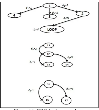
In the second case, the PDG of a program segment is been improved by clustering the control statements such as loop statements into one unbreakable node, which maximizes the chance of finding new acceptable solutions. In this case, the

PDG of a program P will be recreated as shown in

Figure 10. Notice that the SS-CRO algorithm will not be allowed to break up the loop statement. In other words, control dependency will be excluded

from the PDG, which will increase the chance of

finding more accepted solutions.

In the third case, the PDG is been improved more than the second case, where dependent nodes have been clustered in one unbreakable independent component. In Figure 18, nodes 1-4 and the loop

node have been clustered in Comp1, nodes 11-14

have been clustered in Comp2, and nodes 15-17

have been clustered in Comp3.

In this improvement, all kinds of dependencies

have been excluded from the PDG, which increases

the chance of finding more acceptable solutions,

because of the reduction of PDG’s restrictions, i.e.

instructions’ dependencies.

Furthermore, the SS-CRO algorithm is

compared with two distinct optimization

algorithms, which is static scheduling based on genetic algorithm is denoted as SS-GA, where it is implemented based on the well-known genetic algorithm presented by authors of [41]. Moreover, static scheduling based on duelist algorithm and denoted as SS-DA, which is implemented based on the recent known algorithm duelist presented by authors of [44]. The input of the three algorithms

will be the same, which it is the PDG of a program

segment in its three cases as shown above.

In SS-GA algorithm, the scenario of the algorithm is inspired from the well-known genetic algorithm posited in [41], which will be explained

as follows. First, SS-GA takes the PDG and

generates random population of chromosomes (a chromosome is a binary vector that reflects the

dependencies between the PDG nodes) by

3159 then it applies the crossover function over them to get the new offspring. Third, SS-GA calls the fitness function for each chromosome (the fitness function here checks all nodes dependencies in the

chromosome relates to their PDG). Forth, SS-GA

uses a probability of mutation to mutate the nodes of the new offspring. Fifth, SS-GA places the new offspring in the population, after it is been accepted (i.e. preserves the nodes dependencies). This process will be repeated until the algorithm is been terminated according to the number of iterations.

In SS-DA algorithm, the scenario of the algorithm is inspired by the duelist algorithm posited in [44], as follows. First, SS-DA generates a random population by reordering the PDG nodes the same way as SS-GA, see the above paragraph. Second, SS-DA choses two duelist then it computes the luck variable, which is done using the dependency between the nodes some random numbers for each duelist. The luck of each duelist will be compared and the winner will have the better luck. Third, SS-DA treats the winner and a new solution will be added to the solution list, and then SS-DA returns the looser back to the population to give it a chance to reenter the competition. SS-DA will repeat the process according to its number of iterations

P′1

Instructions Cost(d)

11: DIV.D F9,F10,F11; 0 12: ADD.D F12,F9,F10; 2 13: SUB.D F13,F12,F11; 2 14: MUL.D F13,F12,F11; 3 1: DIV.D F1,F2,F3; 0

2: ADD.D F2,F4,F1; 2

3: SUB.D F5,F1,F6; 1

4: MUL.D F7,F1,F8; 1

5: LOOP: L.D F0, 0(R1); 0 6: ADD.D F4,F0,F2; 2 7: S.D F4, 0(R1); 2

8: DADDUI R1,#-8; 1

9: BNE R1, 1

10: LOOPEND; 0

15: MUL.D F14,F15,F16 0

16: ADD.D F15, #8 1

17: MULD. F14,F15,F16 3

Total 20

(a) P′1 program segments

(b) PDG of P′1

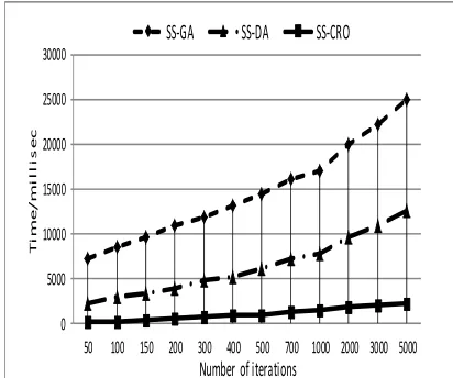
Figure 9: A valid solution based on reordering approach

Figure 10: PDG in the second case