AUTOMATIC SPOKEN LANGUAGE RECOGNITION FOR MULTILINGUAL SPEECH RESOURCES

8244

A COMPARATIVE STUDY ON THE SOFTWARE

ARCHITECTURE OF WRF AND OTHER NUMERICAL

WEATHER PREDICTION MODELS

ABEDALLAH ZAID ABUALKISHIK

American University in the Emirates, College of Computer and Information Technology, Dubai, United Arable Emirates (UAE).

E-mail: [email protected], [email protected]

ABSTRACT

Software modularity architecture facilitates software development and software reusability. Software reusability enhances the maintenance of software, facilitates building larger component out of sub-components. Numerical weather prediction uses complex mathematical models and run them on powerful computers to forecast weather conditions. Numerical weather prediction models have proliferated and can be classified into regional and global models. The Weather Research Forecast model is considered the next-generation mesoscale regional model and widely used. The Weather Research Forecasting model consists of several modules interacting with each other. This research aims to study the WRF’s software architecture, software modules, and the forecasting accuracy of WRF in respect to other well-known Numerical Prediction Models. The study outcomes show that WRF’s software architecture characterized with high degree of flexibility, loosely coupled modules which plays a very important role to obtain accurate forecasting results through the application of independent modules, and consequently it provides a high reliable and accurate forecasting results.

Keywords:Weather Research Forecasting, Numerical Weather Prediction, Software Architecture.

1. INTRODUCTION

Numerical weather prediction (NWP) is the process of forecasting future weather parameters based on the current given weather parameters via mathematical models that describe the flow of fluids. NWP calculation requires super computer to forecast weather parameters such as temperature, air pressure, wind speed and direction, rain fall… etc. Usually, NWP aims to predict and simulate atmosphere. Mathematical models can be used to obtain the forecasting at two levels, time span (long term or short term) and geographical area. The later called the Mesoscale meteorology that classifies the forecasted area according to its area scale. There are three subclasses alpha 200-2000 km scale, Meso-beta 20-200 km scale, and Meso-gamma 2-200km scale. Each category aims to study certain event. The accuracy of NWP is subjected to the mathematical models applied and the quality of input data to such models.

Weather Research Forecasting (WRF) that is also known as North American Mesoscale

NAM or WRF Nonhydrostatic Mesoscale Model NMM refers to the software that achieves the purposes of NWP. WRF consists of two main cores, namely, data assimilations and the software architecture that allows for parallel processing and offers extensibility. WRF has been known as the second-generation mesoscale NWP. The main goal of WRF is to produce simulation and forecasting for atmospheric conditions via the observed and analyzed conditions. The two dynamical solvers/cores of WRF that are used to perform the atmospheric governing equations computation are: Advanced Research WRF (ARW) and the NMM. WRF is the results of collaboration between the National Centers for Environmental Prediction (NCEP) that developed the NMM, and National Center for Atmospheric Research (NCAR) developed the ARW. WRF is a community supported model and through worldwide users and officially supported by NCAR and many others [1].

8245 component is a unit of composition with clear interface. The main characteristic of a software component is that it can be deployed and composed by a third party [2]. The key features of a software component are: Encapsulation, Inheritance and Polymorphism.

WRF is an open source software where the code is available to the public and flexible to different configuration, i.e. dynamics, boundaries, physics. WRF uses an architecture that divides its functionalities into many modules and components. Thus, it is easy to maintain, reuse, extensible, flexible and ease of parallelization. There are so many competitive forecasting models for NWP as COSMO, GEM, GFS, RegCM, ECMWF, UKMET, HARMONIE-AROME, and BAM. The goal of this paper is of threefold: Study the architecture of WRF and its advantages and disadvantages. Second goal aims to compare the WRF software architecture and the associated features in respect to other NWP models. Third goal aims to compare the accuracy of WRF with the studied models.

This paper is structured as follows: Section 2 presents the software architecture of WRF, section 3 provides a comparative analysis of WRF and other NWP models and related literature review, and finally section 4 shows the study conclusion.

2. WEATHER RESEARCH

FORECASTING

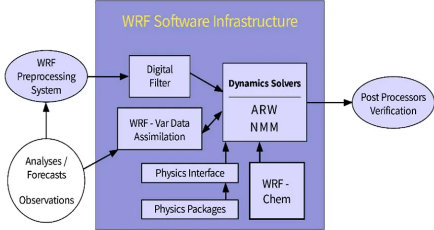
WRF has been developed at Penn state university at NCAR primarily using Fortran and C. It has appeared to overcome the shortcomings exist in the Fifth-Generation Penn State/NCAR Mesoscale Model (MM5). WRF is the results of a collaborative open source software applications and designed to predict numerical weather and simulate atmosphere. The code of WRF reflects the state-of-the-art, flexible code that is optimized to be executed in computing devices that range from super computer to laptop. The development is based on modules. Figure 1 shows the WRF architecture that compromises the main modules [3].

Figure 1:WRF Software Architecture

This architecture applies the principles of layer that promotes the architecture modularity, reusability, flexibility and portability. The principle of abstraction and information hiding are applied too to guarantee parallelism and data management. Thus, this architecture facilitates the initialization and communication of the solvers (ARW, NMM) through physics packages, WRF-Chem, WRF data assimilation and digital

filter. The core of WRF is the solvers and they are: The ARW that is mainly developed at NCAR, and the NMM solver that was developed at NCEP.

8246 analysis or a forecast of real data case for real simulation. WPS main functionality is to convert the large-scale data, i.e. GriB into a suitable format for processioning and manipulation by the ARW’s processors [3]. The next step is to assimilate data from multiple sources. WRF assimilation received multiple types of data like radar and precipitation data and integrate them with the forecast model input preprocessed data to aggregate more data that would produce higher accurate estimation of atmospheric conditions.

The two solvers communicate with the physics package via the physics interface. The physics packages are easily integrated and interchangeable due to the novel design of the physics interface. Accordingly, the physics schema can be easily, relatively, develop in which physicist need to be aware how to implement the algorithm they would like to use and ensure the compatibility of the software with the WRF. The physics schemas are almost equal to the classical definition of software module since it is an independent program that is connected to another program via an interface. Thus, the physics package is easy to develop and maintain, enable composition, and code swapping [4]. The first physics package was imported from the MM5. Currently, there are around 90 physical packages included in the WRF, i.e. Land surface, Ocean option, Urban physics and many others [5].

WRF has been used extensively for several types of research using real data and idealized configuration. The WRF’s functionality can be extended to fulfill other perspectives of weather forecasting like terrestrial forecasting [6], chemistry via WRF-Chem component, tropical cyclones [7], mesoscale weather events and phenomena [8] and many others.

ARW is collaborated with other modules to produce simulations. The ARW along with NMM shares the framework and all other modules especially physics package to produce the desired output. The major features comprise in the ARW solver module are the equations, prognostic variables, vertical coordinate,

horizontal grid, time integration and many others. The physics module includes microphysics schema that is fit for simple to sophisticated physics studies and NWP. Other features like cumulus parameterization, surface physics that concerns with land surface model, and so many others. WRF-Chem component contains some features like the online model to guarantee the consistency of data. Dry decomposition, biogenic emission and so many others.

The WRF software framework facilitates the overall communication, integration and compatibility of all the components together. This framework characterized with high modularity and maintainability via a single-source code. Highly portable across various platform. Supporting various data format via various I/O Application Program Interface (API) that enable multi packages to work with WRF, and efficient execution time [3].

8247

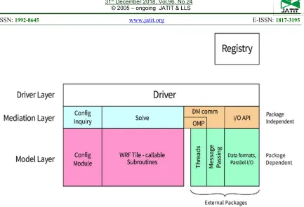
Figure 2: WRF Software Architecture Layers Mode

The WRF was developed using Fortran 90 and C++ in which the modern programming features were there. For example, modules, derived data type, recursion, and dynamic memory allocation. A good design requires avoiding arrays to improve the performance, and so the WRF does. Parallelism is achieved via two level of decomposition through subdividing the model domain into patches and then further subdivided into tiles. Usually, patches are assigned to a distributed memory node, and tiles are allocated to shared memory processor [11]. Indeed, the WRF architecture and the decomposition approach improve software reusability and enhance performance among various platform.

Maintain and managing the source code for such a big project is an issue. Registry is simply a text file that acts as an active data dictionary for the WRF that comprises a record of tables relating to the state of the various data structures of WRF and their attributes, i.e. type, number of time levels, staggering and so many others. Usually, it is called during the compile time to automatically produce the needed interfaces between driver and model layers [11]. Scientists manipulate the state of model by means of modifying registry state without any prior knowledge of model coding, thus, it saves scientist time and reduce the possibility of errors.

Approximately, 20% of the WRF’s code is generated via the registries.

3. WRF AND OTHER NWP MODELS

This section aims at comparing the WRF with the most well-known used NWP models. Indeed, it is difficult to directly compare forecast models since the architectures and mathematical models are different, data from multiple forecast sources can’t be easily compared, furthermore, it is usually rare to perform forecasting using two different forecasting models at the same time and mesoscale. WRF has been widely studied and well documented. Indeed, some models have poor documentation and some has no published documentation. Nevertheless, the available published data has the merit to achieve the objectives of this study.

3.1 WRF vs. COSMO

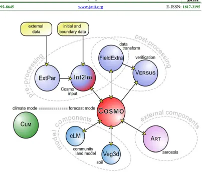
The Consortium for Small-scale (COSMO) is a NWP that aims to develop and maintain a non-hydrostatic small area atmospheric model for research and operation of consortium members [12]. Figure 3 shows a high-level software architecture model of COSMO and several programs. For example, INT2LM concerns with preparing the data for the COSMO model. COSMO itself is the forecasting model. Full details about this model can be found in [12]

8248

Figure 3: The COSMO high software architecture

COSMO model is a limited area nonhydrostatic prediction model designed for research application and NWP. The later mode requires several utilities as data assimilation and interpolation of boundary conditions from a driving model. COSMO model has been evolved since the first release from COSMO 1, COSMO-E and now COSMO 7.

COSMO is a monolithic model with less number of modules and few number of physics parametrization option unlike WRF. Fig 3 shows that the number of modules used by COSMO is far less than WRF. Mainly, the components in COSMO are used for pre and post processing.

Oberto et al. [13] verified the numerical results of COSMO I7 (developed by COSMO) and WRF-NMM over the Italian territory between 2007-2008 at almost 7 km resolution. The results of the study showed that WRF has a general tendency of overestimation for low threshold

unlike COSMO I7 that tends to overestimate for all threshold. The study found certain anomalies which they believe it is due to lack of data assimilation. Mugume et al. [14] compared WRF and COSMO to evaluate the two models ability to predict light and extreme rainfall events over Uganda using a parametrization configuration with horizontal resolution of 7 km. The results show that COSMO tends to under-prediction of no rain prediction and show greater magnitude or error comparing to WRF. However, COSMO performed significantly better than WRF of predicting light rain fall.

3.2 WRF vs. GEM

8249 both models are comparable as long as they are applicable for certain mesoscale. The GEM is running twice a day on its uniform configuration to perform the medium range weather forecast.

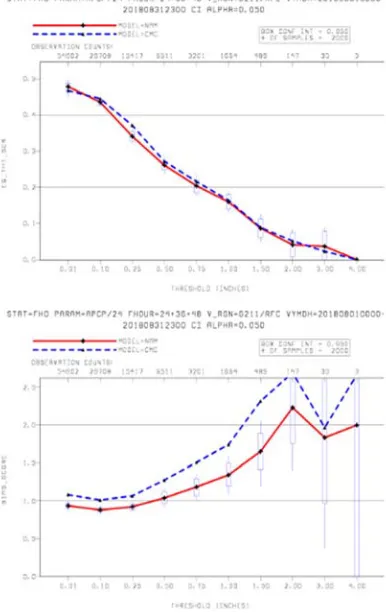
The National Weather Service (NWS) gathers the results regional and global models and compare them. We are interested to see the comparison between CMC’s GEM and North American Mesoscale Forecast System (NAM). Figure 4 shows the comparison for precipitation on August 2018 [15].

Figure 4: GEM and NAM comparison for precipitation over August 2018 [15]

The graph shows NAM’s GEM in red and CMC’s GEM in blue. The upper figure shows threat score and lower figure shows bias. One is the perfect score value for both models. As usual, the WRF model has less bias value than GEM and almost an identical Equitable Threat Score (ETS) that measures the quality of the prediction model.

Wedam et al. [16] inspected the errors in sea level pressure for three 5-month cold season at the united states east and west coast for several NWP models, in particular, the European Centre

for Medium-Range Weather Forecasts (ECMWF), NAM, WRF-NMM, National Centers for Environmental Prediction (NCEP) and GEM. The study found that ECMWF was the most accurate model while NAM was the least accurate. GEM’s accuracy was improved and was in between.

3.3 WRF vs. GFS

The Global Forecast System (GFS) developed by the NCEP is composed of four sub-models (atmosphere, ocean, soil and sea) that collaborate to predict the weather accurately. It covers the whole world with a base horizontal resolution of 28 km. Since GFS is a global mesoscale model it would be probably to underperform WRF that runs at a higher resolution “small mesoscale”. Thus, it is worth to examine this assumption. That is, if the global model is as accurate as the regional model then there is no need to run the later. In particular, when the regional model relies on global model to obtain data as the case of MM5 and NAM do on GFS.

The NCEP/EMC publishes [17] compares between the GFS and NAM with more available measures than it does with NAM and GEM. In particular, it plots bias and root-mean-square error (RMSE). Figure 5 shows a comparison of three models, in principle they are two as the Rapid Refresh model RAP is a WRF with higher resolution and dedicated for short term.

8250 Figure 5 shows that the GFS is the least biased model with values closer to zero comparing to the other two models. The same is applied to the RMSE. It is possible to claim that for this period of time and according to the given data that GFS has outperformed the other two models.

Yan et al. [18] compared the GFS, WRF and NAM for quantitative precipitation short term forecasting (12 hours) at Iowa for a small domain with 4km grid spacing for 9 months. The results show that NAM had the worst results for model skill and spatial feature attributes. Furthermore, finer resolution has not improved the accuracy of

NAM’s WRF for small scale storms compared to GFS. The study found that WRF achieved the best results.

3.4 WRF vs. RCM

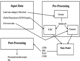
The Regional Climate Model (RCM) is an open source climate model of higher resolution than global models. RCM applies downscaling to obtain high resolution weather information via obtaining better representation of underlying topography at a scale of 50 km or less. RCM just like WRF is maintained via community and supported by the Center for Theoretical Physics. Figure 6 shows the architecture of RCM

Figure 6: RCM model architecture

The RCM process divided into pre-processing to handle input data, the main model where the equations are there to forecast the various weather parameters, the post-processing to generate the output data. The pre-processing component is the terrain file that handles input data and used to create localized topography, land used category information and projection information. Each file contains certain set of data,

for instance, the initial/ lateral boundary condition ICBC files contain temperature, surface pressure and horizontal wind component. The post processing of RCM architecture produces four files in the output directory: ATM holds atmosphere status of the model, SRF contains variables of surface diagnostic, RAD contains radiation information, and CHM that deals with chemical parameters.

8251 has the ability to easily apply rapid development and to adapt itself to other platforms like Earth System Modelling Framework (ESMF). However, RCM can’t apply rapid development or even adapt to other platforms. Moreover, WRF has several physics schemas as shown before while RCM has fewer. Both WRF and RCM are non-hydrostatics models. WRF supports coupling between little number of modules, i.e. ocean and temperature. RCM offers coupling among larger number of components.

3.5 WRF vs. MM5

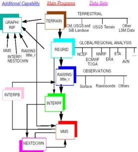
As mentioned earlier, the WRF has appeared to overcome the shortcomings of MM5. MM5 is a regional mesoscale weather and climate forecasting model. It is maintained by Penn State University and the NCAR and considered as a community model. MM5 is a limited area and a hydrostatic/non-hydrostatic model designed to forecast mesoscale and regional atmospheric flow [19]. Figure 7 shows the schematic diagram of MM5.

Figure 7: MM5 Schematic Diagram

MM5 was written in Fortran language, just like WRF, and it needs to be compiled every time there is a configuration change. MM5 is a multitasks software in which parallelism is taken into design consideration and it applies nesting as well [20].

The MM5 composed of eight main modules: TERRAIN deals with input data that defines model domain, then it creates map

8252 NESTDOWN produces input mesh model and produces the output from MM5 in high resolution. INTERPM interpolate model sigma data to pressure level, and finally, GRAP/RIP produces plots and figures [19].

Several studies compared the performance of MM5 and WRF. Kusaka et al. [21] conducted a comparison between WRF and MM5 models to evaluate the performance of rainfall forecast at Baiu Front. The results show that both models barely met the observation. The MM5 forecasted the heaviest rainfall on offshore whereas WRF was onshore. This difference refers to vertical velocity field in which the WRF’s vertical velocity field is more detailed than MM5.

Lie and Warner [22] compared MM5 to WRF to achieve a smooth transition from MM5 to WRF, semi operational forecasts were conducted two times a day with the exactly same resolutions and domains. The results showed that WRF owns same features as MM5 forecasting different mesoscale weather. WRF found to better forecast upper troposphere circulation than MM5 does. On the other hand, MM5 found to produce better results at surface and lower troposphere which

they justify due to the usage of Noah land surface model that characterizes MM5.

3.6 WRF vs. ECMWF

The ECMWF was established in 1975 to fulfill the needs of accurate weather forecast. It is an independent organization that is deployed in European union. It is well known as the most accurate global forecasting model and has one of the largest supercomputer and metrological data archive in the world [23]. The ECMWF developed their own numerical model and data assimilation system which they called the Integrated Forecasting System (IFS). The quality of IFS forecast is limited to the fact of chaotic atmosphere. Therefore, the ECMWF applies probabilistic forecasting [24].

The IFS comprises of several sub-systems coupled together in various several ways: global atmospheric model that controls the resolution of forecasting, ocean wave model, dynamic ocean model, atmospheric model data sources, model data assimilation, and the continuing sequence of analysis. Figure 8 shows the ECMWF IFS physical quantities exchange that is tightly related to the software architecture [24].

8253 Bauer et al. [23] investigated the quantitative precipitation estimation and forecasting between WRF and ECMWF over central Europe. The comparison conducted over a 1-hour rapid update cycle with data from multiple resources as the French radar system, the European GPS network and satellite sensors. The comparison was verified qualitatively and quantitatively. The results detected a significant improvement in the WRF model using downscaling comparing to a reasonable performance of ECMWF.

4. CONCLUSION

This study investigated the software architecture of the most well-known numerical weather prediction forecasting models in respect to the WRF model. The study found that the WRF model provides a reliable and trusted results in the community by comparing it to the well-known used models. The architecture of WRF provides an advantage over other models.

The study found that WRF used to provide higher accurate results than the other models. However, it is impossible to claim that it is the best as weather forecasting is chaotic and unstable. Indeed, WRF found on several places to outperform other models. The performance of WRF results are most likely related to the solvers, and the software architecture that is based on separate software modules. In particular, the physical modelling and data assimilation that are completely independent from the model’s core. To conclude, WRF is among the most widely used regional forecasting model. The WRF’s software utilities architecture plays an important role to achieve this reputation, in addition to the large number of WRF’s community and the data availability.

REFERENCES

[1] J. G. Powers et al., “The weather research and forecasting model: Overview, system efforts, and future directions,” Bull. Am. Meteorol. Soc., 2017.

[2] M. Broy et al., “What characterizes a (software) component?,” Softw. - Concepts Tools, 1998.

[3] W. C. Skamarock et al., “A Description of the Advanced Research WRF Version 3.” 2008. [4] J. L. Coen, M. Cameron, J. Michalakes, E. G.

Patton, P. J. Riggan, and K. M. Yedinak,

“Wrf-fire: Coupled weather-wildland fire modeling with the weather research and forecasting model,” J. Appl. Meteorol. Climatol., 2013.

[5] “WRF Model Physics Options and References,” 2018. [Online]. Available: http://www2.mmm.ucar.edu/wrf/users/phys_r eferences.html#TOP.

[6] Y. Zhang, J. Hemperly, N. Meskhidze, and W. C. Skamarock, “The Global Weather Research and Forecasting (GWRF) Model: Model Evaluation, Sensitivity Study, and Future Year Simulation,” Atmos. Clim. Sci., 2012.

[7] Y. Zhang, J. A. Smith, A. A. Ntelekos, M. L. Baeck, W. F. Krajewski, and F. Moshary, “Structure and Evolution of Precipitation along a Cold Front in the Northeastern United States,” J. Hydrometeorol., 2009.

[8] J. J. Shi et al., “WRF simulations of the 20-22 January 2007 snow events over eastern Canada: Comparison with in situ and satellite observations,” J. Appl. Meteorol. Climatol., 2010.

[9] Mesoscale & Microscale Meteorology Division / NCAR, “WRF Modeling System Overview.” 2010.

[10] J. Michalakes et al., “the Weather Research and Forecast Model : Software Architecture and Performance,” Use High Perform. Comput. Meteorol. Proc. Elev. ECMWF Work., 2004.

[11] J. Michalakes et al., “Development of a Next Generation Regional Weather Research and Forecast Model,” Proc. Ninth ECMWF Work. Use High Perform. Comput. Meteorol., 2001. [12] Consortium for Small-scale, “COSMO,” 2016. [Online]. Available:

http://www.cosmo-model.org/content/model/default.htm. [13] E. Oberto, M. Milelli, F. Pasi, and B. Gozzini,

“Intercomparison of two meteorological limited area models for quantitative precipitation forecast verification,” Nat. Hazards Earth Syst. Sci., 2012.

[14] I. Mugume et al., “A Comparative Analysis of the Performance of COSMO and WRF Models in Quantitative Rainfall Prediction,” World Acad. Sci. Eng. Technol. Int. J. Mar. Environ. Sci., vol. Vol:12, no. 2, 2018. [15] National Centers For Environmental

8254 “NCEP/EMC Precipitation Skill Scores for Operational Models,” 2018.

[16] G. B. Wedam, L. A. McMurdie, and C. F. Mass, “Comparison of Model Forecast Skill of Sea Level Pressure along the East and West Coasts of the United States,” Weather Forecast., 2009.

[17] National Centers For Environmental Prediction’s Environmental Modeling Center, “EMC MODEL FORECAST VERIFICATION STATS,” 2018. [Online]. Available:

http://www.emc.ncep.noaa.gov/mmb/mmbpll /mmbverif/.

[18] H. Yan and W. A. Gallus, “An Evaluation of QPF from the WRF, NAM, and GFS Models Using Multiple Verification Methods over a Small Domain,” Weather Forecast., 2016. [19] MM5 Community Model, “MM5 Community

Model.” 2018.

[20] MM5, “Section 2: MEMORY ORGANIZATION & CODE STRUCTURE,” 1994.

[21] H. Kusaka, A. Crook, J. Dudhia, and K. Wada, “Comparison of the WRF and MM5 models for simulation of heavy rainfall along the Baiu Front,” SOLA, 2005.

[22] Y. Liu1 and T. Warner, “COMPARISON OF THE REAL-TIME WRF AND MM5 FORECASTS FOR THE US ARMY TEST RANGES.” National Center for Atmospheric Research /RAP.

[23] H.-S. Bauer et al., “Quantitative precipitation estimation based on high-resolution numerical weather prediction and data assimilation with WRF – a performance test,” Tellus A Dyn. Meteorol. Oceanogr., vol. 67, no. 1, p. 25047, Dec. 2015.