8399
PERFORMANCE OF SIGNAL SIMILARITY MEASURES
UNDER 1/F NOISE
ZAINAB H. ALMAHDAWIE, ZAHIR M. HUSSAIN
University of Kufa, Faculty of Computer Science & Mathematics, Najaf, Iraq
E-mail: 1[email protected] , 2[email protected]
ABSTRACT
In this work we present a study on the performance of signal similarity measures under non-Gaussian noise. Pink noise has been considered, with 1/f power spectral density. This kind of noise has been generated by filtering Gaussian noise through an FIR filter. One-dimensional and two-dimensional signals have been considered. We tested 2D image similarity using the well-known similarity measures: Structural Similarity Index Measure (SSIM), modified Feature-based Similarity Measure (MFSIM), and Histogram-based Similarity Measure (HSSIM). Also, we tested 1D similarity measures: Cosine Similarity, Pearson Correlation, Tanimoto similarity, and Angular similarity. Results show that HSSIM and MFSIM outperform SSIM in low PSNR under pink noise and Gaussian noise. For 1D similarity, it is shown that Cosine Similarity and Pearson Correlation outperform other 1D similarity, especially at low SNR.
Keywords: Gaussian Noise, Pink Noise, FM, SSIM, HSSIM, MFSIM, Image Similarity, Cosine Similarity, Tanimoto Similarity, Angular Similarity, Pearson Coefficient.
1. INTRODUCTION
Signal similarity plays a significant role in many applications like Pattern recognition, Face recognition, Signal detection etc. There are many measures for one-dimensional (1D) signals, most important are cosine similarity, Tanimoto similarity, angular similarity and Pearson correlation. For 2D signals (images), there are many similarity measures like SSIM [1], HSSIM [2], and FSIM [3].
The similarity is the amount that mirrors the connection quality among the two components. The measures of similarity have a coefficient range from 0 to 1 [4].
Image similarity measures enable
categorized into statistical and information theoretic [2]. Statistical Methods worthy information can be acquired from the image by calculating statistical sizes such as mean, variance and standard deviation. This information can be utilized to calculate image similarity [1]. The information-theoretic method is targeted to find the similarity among images affording to their content (intensity values) [5].
In this work, we will investigate the performance of 1D and 2D similarity measures under 1/f Noise. This kind of noise is very important because it used in electronics and audio
[6], several physical systems such as
communication channels [7], electronic
components and semiconductors devices [8,9], natural phenomena (e.g., rivers, ocean flows, average seasonal temperature, rainfall) [10], financial markets [11], image [12], acoustics and music [13].
The study of pink noise as an entity began in the first half of the 20th century. In 1925, Johnson found frequency dependent noise whose spectral density increased with decreasing frequency [14].
Colored noise denotes to any broadband noise with a non-white Spectrum. Also, a white noise transient done a channel is “Colored” by the form of the channel spectrum. Two classic changes of colored noise are named as pink noise and brown noise [15].
8400 distance, for 1/f noise samples are strongly correlated even at long time distance.
The paper is ordered as follows: Section 2 deals with similarity measures. Section 3 presents a generated and analysis of pink noise. In Section 4 test environment performance measures over two type noise. Finally, in Section 5 conclusions of this study.
2. RATIONALE
Pink noise has been under attention of researchers in the last two decades due its major effects on electronic systems for signal and image processing [6,16,17]. To the best of our knowledge, there is no work so far that focuses on evaluating similarity measures under 1/f pink noise. Hence, we handled this task for 1D and 2D signal similarity measures.
3. SIMILARITY MEASURES
In this section we review some of the most effective signal similarity measures for 1D and 2D signals.
3.1 Structure Similarity Index Measure
Structure Similarity Index Measure (SSIM) is a statistical measure using statistical image parameters such as mean, variance, co-variance, and standard deviation [1, 18]; it is defined in Equation (1)
(1)
where is the similarity metric between
images and , while , , and are the
statistical means and variances of and ,
respectively; is the covariance of and , and
lastly the constants and are injected to avoid unstable results that may be reached due to division
by zero, and are defined as = and
= , with and are tiny small positive
constants and (extreme pixel value).
3.2 HSSIMMeasure
One of the effective image similarity measures is based on information-theoretic properties via the histogram is the Histogram-based similarity measure (HSSIM) [2, 19]. It is proposed to deal with the problem that SSIM measure can't perform well under significant noise. HSSIM depends on information-theoretic properties by using the joint histogram. HSSIM utilizes a normalized form of joint histogram [2, 19]. Equation (2) explains this measure.
(2)
where is the HSSIM measure,
is the original image histogram, is the joint
histogram, and is a small positive constant to keep away from division by zero.
3.3 Feature Similarity Index Measure
Feature Similarity Index Measure (FSIM) is a quality assessment measure relying upon human vision system (HVS) which understands an image in a general sense. The phase congruency (PC) is used as the primary property.
PC is a dimensionless measure to quantify the importance of a neighborhood structure; while the gradient magnitude (GM) is utilized as the subordinate property [20]. The calculation of the FSIM involves two steps. In the first step, the PC and GM characteristics will be isolated using gradient operators, the Prewitt operator, the Sobel operator, and the Scharr operator [21]. The
similarity measure for PC rates SPC(x) and GM
values SG(x) are well-defined in Equations (3) and
(4) below:
(3)
(4)
The second step is to calculate the as
follows:
(5)
where means the whole image spatial domain.
Finally, one calculates the as
Equation (6):
8401 However, FSIM gives non-zero values for non-similar images, therefore we propose a modification called MFSIM as follows:
(7)
3.4 Cosine Measure
Cosine similarity has been commonly utilized for the similarity measurement between two 1D signals [22]. Cosine similarity measure is defined as the internal product of two signals divided by the product of their lengths [23, 24]. The
cosine similarity between two signals is
defined in Equation (8) [22]:
(8)
3.5 Tanimoto Measure
The computation of similarity between two signals is then an issue of quantifying, by some suitable measure, the similarity between their particular features. One of the most commonly utilized similarity measures using geometric properties is the Tanimoto coefficient [25, 26]. It has been normally used as a genuine measure of
intermolecular comparability. Given two signals A
and B, Tanimoto measure is defined as follows:
(9)
where stands for the dot product.
3.6 Angular Measure
The angular distance between two signals
can be utilized to measure similarity. The angular measure is defined as follows:
(10)
The angular distance which measures the orientation change between two signals is a significant measure of their similarity [27, 28].
3.7 Pearson Correlation Coefficient Measure The Pearson correlation coefficient of two
signals and is accurately described as the
covariance of the two factors divided by their
standard deviations (which works as a
normalization factor); it can be suitably described by [29]:
(11)
where
(12)
and
(13)
where is the signal length. The coefficient ranges from 0 to 1 and it is invariant to direct
changes of the two signals. The gives a sign
on the direct relation between the two arbitrary signals and . If the signals are directly related the sign of the correlation coefficient is positive.
If , and are said to be unrelated [30].
4. GENERATION OF 1/f PINK NOISE
Pink noise is the name given to random signals that contain constant power per percentage bandwidth for all frequencies [31]. Pink noise can be quantified as a signal with power spectral density inversely proportional to the frequency of the signal. In science the term pink noise can loosely be used to represent any signal with power spectral density following Equation (14) with range
of constant (α) between zero and two ( ),
where we get white noise for , pink noise
with , and brown noise with , where f
represents frequency content of noise [6].
(14)
8402
The main feature of 1/f noise is that its
power spectrum increases with decreasing
frequency f down to the lowest possible frequencies
[32, 33].
In this section we generate pink noise by passing white Gaussian noise through FIR filter. Filter order can be used to change the bandwidth of the colored noise and has an effect on performance.
4.1 Gaussian-Distributed Noise’
Gaussian noise is equitably disseminated over the signal [34]. This means that every pixel in the noisy image is the totality of the actual pixel value and an arbitrary Gaussian distributed noise value. This kind of noise has a Gaussian distribution, which has a probability distribution function described in Equation (15) [35]:
(15)
where represents the grey level, is
the mean value and is the standard deviation.
4.2 Finite Impulse Response (FIR) Digital Filter
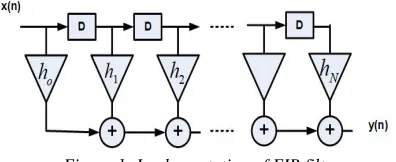
In FIR digital filters their impulse response has a limited number of non-zero samples. In a digital system, the function of the causal FIR filter is given by the following difference equation [36], also shown Figure (1):
(16)
where represents for simplicity. Taking the
z-transform of both sides we get:
(17)
Hence, the transfer function is given by Equation (19):
(18)
From the difference Equation or from the transfer
function we can implement causal finite
impulse response filter by utilizing delay elements and digital multipliers as in Figure 1.
If FIR filter coefficients are symmetric,
then the filter will have linear phase, a feature that is desirable to avoid any signal distortion.
[image:4.612.316.514.284.365.2]A linear-phase FIR filter can be designed by minimizing the weighted integrated squared error between an ideal piecewise linear function and the magnitude response of the filter over a set of desired frequency bands. On MATLAB, this process is done using firls function.
Figure 1: Implementation of FIR filter.
4.3 Effect of FIR filter on White Noise
When a random signal enters a system ,
the output signal would also be random, with power spectral density (PSD) = input PSD multiplied by the power transfer function of the system, which is
Now assume white noise input with
constant PSD entering an FIR filter. The output noise PSD is given by:
(19)
4.4 Pink Noise Generation:
We modeled and analyzed colored pink noise (1/f) as follows:
1. Specify the power of the additive white
Gaussian noise (AWGN), number of realizations, number of samples,
normalized frequency step, and
normalized frequency vector (v=0:1).
2. Design the FIR-filter coefficients required
to produce the necessary pink noise, where need some parameter such as filter order (n) with n+1 coefficients and magnitude
response of , where s is a
8403
3. We used Least squares FIR design,
supported by MATLAB function firls: b=firls(n,v,am).
4. Generate additive white Gaussian noise
(AWGN) by using the MATLAB function randn: u=randn (1, N).
5. Pass the AWGN noise ( ) through the
FIR-filter by using the “filter” function in MATLAB, which convolves the signal with the impulse response of the filter: , with a=1, performing the convolution:
6. Make pink noise have zero mean: subtract
from it the value .
7. For this noise, make variance equal =1:
divide by .
8. Assign the power P to the generated noise
via .
9. To find the spectrum , apply Fourier
transform to noise .
After generating pink noise, it is added to signals to test similarity between two signals using different measures under pink noise.
5. TEST ENVIRONMENT
Two types of noise have been considered in testing and simulation: white Gaussian noise, which is one of the most common noise types encountered in communication systems; and pink noise, which is common in image processing and signal processing systems. To test the performance of similarity measures under pink noise (as compared with Gaussian noise), different categories of images have been considered, also different categories of signals have been considered: linear FM (LFM) and quadratic FM (QFM).
Frequency-Modulated (FM) Signals
A signal whose frequency is variating with time is called FM signal, where FM manner is imprinting data (digital or analog) onto wave which has alternating-current (AC) and no data by varying instantaneous frequency (IF) of this carrier wave. According to the type of data, there are digital modulation and analog modulation [37].
The instantaneous frequency IF is the principal property that characterizes nonstationary signals (fundamental data passed on). Hence, forth IF
estimation is of essential significance in getting data from these signals [38].
We use two types of frequency modulation are a linear frequency modulation (LFM) and quadratic frequency modulation (QFM). In this work, the LFM signal is a law [37,38].
(20)
Where is the amplitude, and is the angle
function for the LFM signal which can be used to calculate the instantaneous frequency of our signal:
and radians/sec.
This means that the instantaneous frequency in Hertz can be given by:
(21)
which leads us to set the angle function as follows:
(22)
where 𝛼 is the modulation index. This results in the
final LFM function is given below:
(23)
For quadratic frequency modulation (QFM) the angle function is given as follows:
(24)
where 𝛼 refers to slope parameter of QFM signal
(linear modulation index) and refers to the quadratic modulation index of the FM signal.
This results in the final QFM function given by:
(25)
6. RESULTS AND DISCUSSION
8404
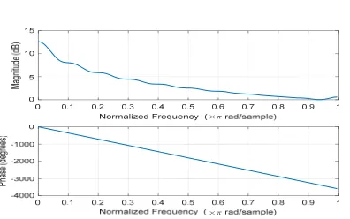
[image:6.612.92.292.262.542.2]Figure 2: Frequency response of the FIR (magnitude and phase).
[image:6.612.326.510.394.477.2]Figure 3: Pink noise versus time.
Figure 4: Spectrum of pink noise.
6.1 Performance of 2D Similarity Measures under Noise
First, we consider the performance of image similarity measures (SSIM, MFSIM and HSSIM) under pink noise. A comparison is shown in Table 1.
In Table 1, MFSIM is better than SSIM and MFSIM improves when m (filter order) goes more than 120. HSSIM gives better more similarity than MFSIM, hence information-theoretic measures are more powerful.
Second, we consider the performance of image similarity measures (SSIM, MFSIM and HSSIM) under white Gaussian Noise. Table 2 shows a numerical comparison.
In Table 2, MFSIM and HSSIM are better than SSIM, HSSIM is better than MFSIM.
A complete comparison under pink noise is shown in Figure 5, while Figure 6 shows a comparison under Gaussian noise.
Figures 7 and 8 show the performance of SSIM, MFSIM and HSSIM using similar images (coins image from MATLAB) under pink noise for different FIR orders (m=150, 50).
Figure 9 shows the performance comparison under Gaussian noise.
Note that in the legends of these figures, the letter p will refer to pink noise, while g refers to Gaussian.
Table 1: SSIM, MFSIM and HSSIM versus PSNR under pink Noise (filter order = m=130; image is peppers from
MATLAB).
PSNR (dB) Similarity measures
SSIM MFSIM HSSIM 30 0.3707 0.9674 0.9990 20 0.1351 0.7903 0.9548 0 0.0062 0.0935 0.2433 -10 0.0015 0.0267 0.0805
Table 2: SSIM, MFSIM and HSSIM versus PSNR under white Gaussian noise (filter order = m=130; image is
peppers from MATLAB).
PSNR (dB)
Similarity measures
SSIM MFSIM HSSIM
30 0.3613 0.9498 0.9990
20 0.1294 0.7207 0.9556
0 0.0059 0.0676 0.2482
[image:6.612.321.512.536.630.2]8405
(a)
(b)
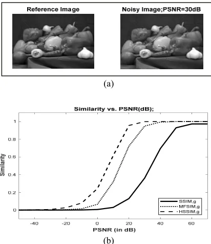
Figure 5: (a) Original image and noisy one with pink noise image (PSNR=30 dB), (b) Performance Comparison of SSIM, MFSIM and HSSIM using similar images (peppers image) under pink noise.
Note: In the legends of these figures, p will refer to pink noise, while g refers to Gaussian.
(a)
(b)
Figure 6: (a) Original image with white Gaussian noise image (PSNR=30 dB), (b) SSIM, MFSIM and HSSIM using similar images (peppers image) under white Gaussian noise.
[image:7.612.90.487.68.349.2]Figure 7: Performance Comparison of SSIM, MFSIM and HSSIM using similar images (coins image) under pink noise (m=150).
[image:7.612.319.517.286.408.2]Figure 8: Performance Comparison of SSIM, MFSIM and HSSIM using similar images (coins image) under pink noise (m=50).
Figure 9: Performance Comparison of SSIM, MFSIM and HSSIM using similar images (coins image) under white Gaussian noise.
From the above results we conclude the following:
1- MFSIM performs better than SSIM under
[image:7.612.90.296.405.643.2] [image:7.612.315.518.477.598.2]8406
2- Under pink noise, SSIM and MFSIM
perform the same as white Gaussian noise, for m<120, m is order of FIR filter.
3- For m>120, MFSIM performs better,
while SSIM stays the same.
4- HSSIM is the best in all cases (white
Gaussian noise or pink noise).
6.2 Performance of 1D Similarity Measures using Noisy FM Signals
Here we consider performance of similarity measures using frequency-modulated signals.
Linear Frequency Modulation (LFM)
[image:8.612.320.521.93.231.2]Performance of cosine, Pearson correlation, angular and Tanimoto measures for LFM under pink noise is shown in Figures 10 and 11 for different FIR lengths.
Figure 10: Performance of cosine, Pearson Correlation, angular and Tanimoto, 10 realizations using similar LFM signal under pink noise (m=10).
Figure 11: Performance of cosine, Pearson Correlation, angular and Tanimoto, 10 realizations using similar LFM signal under pink noise (m=130).
[image:8.612.315.517.356.484.2]Performance cosine, Pearson Correlation, angular and Tanimoto measures for LFM under white Gaussian noise is shown in Figure 12.
Figure 12: Performance of cosine, Pearson Correlation, angular and Tanimoto, 10 realizations using similar LFM signal under Gaussian noise.
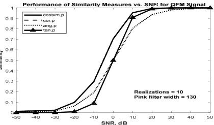
[image:8.612.92.296.373.493.2]Quadratic Frequency Modulation (QFM) Performance of cosine, Pearson Correlation, angular and Tanimoto measures for QFM under pink noise is shown in Figures 13 and 14 for different FIR lengths.
Figure 13: Performance of cosine, Pearson Correlation, angular and Tanimoto, 10 realizations using similar QFM signal under pink noise (m=10).
[image:8.612.321.531.536.659.2] [image:8.612.93.294.537.651.2]8407 Performance of cosine, Pearson Correlation, angular and Tanimoto measures for QFM under white Gaussian noise is shown in Figure 15.
Figure 15: Performance Comparison of cosine, Pearson Correlation, angular and Tanimoto, 10 realizations using similar QFM signal under white Gaussian noise.
Future directions will involve testing similarity measures over modern engineering systems, especially wireless channels as in [39, 40,41] and chaotic communication systems as in [42,43].
7. CONCLUSION:
We presented a detailed study on the performance of 1D and 2D similarity measures under 1/f pink noise. It is shown that 1D and 2D similarity measures exhibit different performance under 1/f pink and Gaussian noise. Pink noise has been under attention in the recent years due its influence on various signal processing systems, while to the best of our knowledge there is no work in the literature to evaluate similarity measures under such kind of noise. It appeared that entropic features of 2D signals (images) are more stable under all kinds of
noise than correlative properties. Hence,
information-theoretic measures (e.g., the recently-proposed histogram signal similarity, HSSIM) outperforms the standard structural similarity SSIM or the feature-based similarity (FSIM). As FSIM exhibits non-zero similarity for non-similar images, we introduced the modified FSIM (MFSIM), which has a performance similar to that of FSIM, except for exhibiting a balanced similarity range from 0 (for different images) to 1 (for identical images) instead of giving spurious non-zero similarity for different images. We presented a method to generate pink noise with 1/f power spectral density using FIR filter with least-squares and linear phase design methods. The condition of linear phase is common in speech processing systems to avoid phase distortion. However, phase distortion could be a future research attempt. We conclude the following about 1D similarity under 1/f pink noise:
1. For any filter order m: Pearson correlation
and cosine similarity outperform Tanimoto and angular similarity (they can detect similarity at lower signal-to-noise ratio, SNR by giving higher similarity for the noisy version of an image at low SNR).
2. At high filter order (e.g., m=130): Pearson
correlation performs better under 1/f pink noise at low SNR than its performance under Gaussian noise. This means that Gaussian noise has more degrading effect than 1/f pink noise.
3. At moderate order (e.g., m=10): Pearson
Correlation shows the same performance under pink or Gaussian at low SNR.
ACKNOWLEDGEMENT:
The Authors would like to thank the Ministry of Higher Education and Scientific Research in Iraq for financial support of this project.
REFRENCES:
[1] Z. Wang, A. C. Bovik, H. R. Sheikh, and
E. P. Simoncelli, “Image quality assessment: from error visibility to
structural similarity,” IEEE transactions
on image processing, vol. 13,4 , 2004, pp. 600-612.
[2] A. F. Hassan, D. Cailin, and Z. M.
Hussain, “An information-theoretic
image quality measure: Comparison with
statistical similarity,” Journal of
Computer Science, 2014.
[3] L. Zhang et al., “FSIM: A feature
similarity index for image quality assessment,” IEEE transactions on Image Processing, 2011. 20(8): p. 2378-2386.
[4] B. Cramariuc, I. Shmulevich, M.
Gabbouj, and A. Makela, “A new image similarity measure based on ordinal
correlation," International Conference on
Image Processing, 2000.
[5] R. Soundararajan and A. C. Bovik,
"Survey of information theory in visual
quality assessment," Signal, Image and
Video Processing, vol. 7,3, 2013,pp. 391-401.
[6] A. Daniel, “Pink Noise in Physics and
Music,” Technical Report, The
University of Nottingham, 2015.
[7] G. Wornell, “Communication over fractal
8408 Acoustics, Speech, and Signal Processing (ICASSP), 1991.
[8] M. S. Keshner, “1/f noise,” Proceedings
of the IEEE, vol. 70, no.3, 1982, pp. 212-218 .
[9] M. Fukuda, T. Hirono, T. Kurosaki, and
F. Kano, “1/f noise behavior in
semiconductor laser degradation,” IEEE
photonics technology letters, vol. 5,10, 1993, pp. 1165-1167 .
[10] H. E. Hurst, “Methods of using long-term
storage in reservoirs,” Proceedings of the Institution of Civil Engineers, vol. 5,5, 1956, pp. 519-543.
[11] B. B. Mandelbrot, “The variation of
certain speculative prices,” in Fractals and Scaling in Finance, ed: Springer, 1997, pp. 371-418.
[12] D. Saupe, “Random fractals in image
synthesis,” in Fractals and Chaos, Springer, 1991.
[13] R. F. Voss and J. Clarke, “1/f noise’’in
music: Music from 1/f noise,” The Journal of the Acoustical Society of America, vol. 63,1, 1978, pp. 258-263 .
[14] P. Dutta and P. Horn, “Low-frequency
fluctuations in solids: 1 f noise,” Reviews
of Modern Physics, vol. 53,3, 1981, p.
497.
[15] S. V. Vaseghi, “Noise and distortion,”
Advanced Digital Signal Processing and Noise Reduction, Second Edition, 2000.
[16] R. Rakhi and S. Shrivastava, “Generation
of Pink Noise using Pseudo Random Binary Sequence,” Technical Report, IIT Bombay, India, 2018.
[17] G. Zanella, “1/f noise from the
coincidences of similar single-sided random telegraph signals,” arXiv preprint physics/0607044, 2006.
[18] Z. Wang and A. C. Bovik, “Modern
image quality assessment,” Synthesis
Lectures on Image, Video, and
Multimedia Processing, Morgan & Claypool Publishers, 2006.
[19] A. F. Hassan, Z. Hussain, and D. Cai-lin,
“An Information-Theoretic Measure for Face Recognition: Comparison with Structural Similarity,” International Journal of Advanced Research in Artificial Intelligence, 2014.
[20] P. Kovesi, “Image features from phase
congruency,” Videre: Journal of
Computer Vision Research, vol. 1,3, 1999, pp. 1-26.
[21] B. Jähne, H. Haussecker, and P. Geissler,
Handbook of computer vision and applications: Citeseer, 1999.
[22] S. Xie and Y. Liu, “Using corpus and
knowledge-based similarity measure in maximum marginal relevance for meeting summarization,” in IEEE Int. Conf. Acoustics, Speech and Signal Processing (ICASSP 2008), 2008.
[23] A. Bhattacharyya, “On a measure of
divergence between two multinomial populations,” Sankhyā: the Indian Journal of Statistics, 1946, pp. 401-406 .
[24] G. Salton, Michael J. McGill, Introduction
to Modern Information Retrieval,
McGraw-Hill, 1983.
[25] T. T. Tanimoto, Elementary Mathematical
Theory of Classification and Prediction, Verlag, 1958.
[26] P. Willett, J. M. Barnard, and G. M.
Downs, “Chemical similarity searching,” Journal of Chemical Information and Computer Sciences, vol. 38,6, 1998, pp. 983-996 .
[27] D. Androutsos, K. Plataniotiss, and A. N.
Venetsanopoulos, “Distance measures for color image retrieval,” International
Conference on Image Processing (ICIP),
1998, pp. 770-774.
[28] D. Androutsos, K. N. Plataniotis, and A.
N. Venetsanopoulos, “A novel vector-based approach to color image retrieval using a vector angular-based distance measure,” Computer Vision and Image Understanding, vol. 75,1-2, 1999, pp. 46-58.
[29] J. Lee Rodgers and W. A. Nicewander,
“Thirteen ways to look at the correlation coefficient,” The American Statistician, vol. 42, no.1, 1988, pp. 59-66.
[30] H. Zhou, Z. Deng, Y. Xia, and M. Fu, “A
new sampling method in particle filter based on Pearson correlation coefficient,” Neurocomputing, vol. 216, 2016, pp. 208-215 .
[31] D. Keele Jr, “The design and use of a
simple pseudo random pink-noise generator,” Journal of the Audio Engineering society, vol. 21,1, 1973, pp. 33-41.
[32] G. Zanella, “1/f noise from the
8409
[33] M. S. Keshner, “1/f noise,” Proceedings
of the IEEE, vol. 70, no.3, 1982,pp. 212-218 .
[34] S. E. Umbaugh, Digital Image Processing
and Analysis: Human and Computer Vision Applications with CVIPtools, CRC press, 2010.
[35] C. Saxena and D. Kourav, “Noises and
Image Denoising Techniques: A Brief
Survey,” International Journal of
Emerging Technology and Advanced Engineering, vol. 4,3, 2014, pp. 878-885.
[36] Z. M. Hussain, A. Z. Sadik, and P.
O’Shea, Digital Signal Processing: An
Introduction with MATLAB and
Applications, Springer, 2011.
[37] Z. M. Hussain and B. Boashash,
“Adaptive instantaneous frequency
estimation of multi-component FM signals using quadratic time-frequency distributions,” IEEE Transactions on Signal Processing, vol. 50, no. 8, August 2002, pp. 1866 –1876.
[38] B. Boashash, Time-Frequency Signal
Analysis and Processing: a
Comprehensive Reference, Academic Press, 2015.
[39] S. S. Mahmoud, Z. M. Hussain, and P.
O'Shea, “Geometrical model for mobile radio channel with hyperbolically distributed scatterers,” IEEE Int. Conf. Communication Systems (ICCS 2002), Singapre, 2002.
[40] S. S. Mahmoud, Z. M. Hussain, and P.
O'shea, “A geometrical-based microcell mobile radio channel model,” Wireless Networks, Springer, vol. 12, 2006,pp. 653-664.
[41] A. K. Gurung, F. S. Al-Qahtani, Z. M.
Hussain, and H. Alnuweiri, “Performance analysis of amplify-forward relay in mixed Nakagami-m and Rician fading channels,” in IEEE Inter. Conf. Advanced
Technologies for Communications
(ATC), 2010.
[42] Y.-S. Lau and Z. M. Hussain, “A new
approach in chaos shift keying for secure communication,” IEEE Inter. Conf.
Information Technology and
Applications (ICITA), Sydney, Australia, 2005.
[43] Y.-S. Lau, K. H. Lin, and Z. M. Hussain,
“Space-time encoded secure chaos
communications with transmit
beamforming,” in IEEE TENCON, Melbourne, Australia, 2005.