ORIGINAL RESEARCH ARTICLE
DYNAMICS OF FOREST DEFORESTATION IN THE AMAZON OF PARÁ: AN APPROACH
CENTERED IN SPACE ECONOMETRY
1,
*André Cutrim Carvalho,
2Raimundo Nelson Souza da Silva,
3Gisalda Carvalho Filgueiras,
4
Abner
Vilhena
de
Carvalho,
5Tatiana Pará Monteiro
de
Freitas and
6Elisabeth Dos Santos
Bentes
1
Professor at The Faculdade de CiênciasEconômicas (FACECON) Andon The Programa de Pós-Graduaçãoem
Gestão de Recursos Naturais e Desenvolvimento Local na Amazônia/Núcleo de MeioAmbiente
(PPGEDAM/NUMA) at The Universidade Federal do Pará (UFPA)
2
Professor at The Universidade Federal Rural da Amazônia (UFRA)
3Female Professor at The FACECON/ICSA/UFPA
4
Professor at The Universidade Federal do Oeste do Pará (UFOPA)
5Female Professor at TheInstituto Federal do Pará (IFPA)
6Female Professor at The Universidade da Amazônia (UNAMA)
ARTICLE INFO ABSTRACT
This article aims to theoretically discuss the main factors responsible for the dynamics of forest clearing in the Amazon of ofPará, an approach perspective performed through spatial econometrics. The basic hypothesis is that the expansion of the agricultural frontier is the conductive element from forest deforestation phenomenon in Pará. In this context, the spatial econometrics served as an extremely important tool to measure, from the results obtained in spatial econometric model the effects that the forest clearing has led in Pará. The main conclusion is that the increased expansion of cattle ranching in the Amazon frontier driven by demand from abroad has directly influenced the increase of deforestation, hindering the development of sustainable activity in the region.The period chosen for the spatial econometric analysis covers the years 2000 and 2008 due to high forest deforestation rate in the state of Pará.
Copyright © 2018,André Cutrim Carvalho et al. This is an open access article distributed under the Creative Commons Attribution License, which permits unrestricted use, distribution, and reproduction in any medium, provided the original work is properly cited.
INTRODUCTION
Over the past decades there has been a growing and continuous modification of the Amazon rainforest caused by high rates of deforestation, which culminated in a significant loss of forest cover, given the extent of the affected land. In this context, fires resulting from forest deforestation process are causing three problems that directly affect all involved there biodiversity, after all, cause air pollution due to the large clouds of smoke that come to cause respiratory diseases we humans, degradation increasing soil, including erosion, constant hydrological cycle and especially the destruction of biodiversity.
*Corresponding author: André Cutrim Carvalho,
Professor atthe Faculdade de Ciências Econômicas (FACECON) andonthe Programa de Pós-Graduação em Gestão de Recursos Naturais e Desenvolvimento Local na Amazônia/Núcleo de Meio Ambiente (PPGEDAM/NUMA) atthe Universidade Federal do Pará (UFPA)
In addition, the effect of forest deforestation ends up affecting economic productivity and causes other disorders of ecological nature. But from the deforestation of cover crops, the disappearance of tropical rainforests, has become the biggest concern, as is happening at a very fast pace, endangering their economic and ecological functions. With an area of more than 1.5 billion hectares, the tropical rainforests are the richest ecosystems in biomass and biodiversity existing in the world, with approximately two-thirds of the humid tropical forests are in Latin America, especially in the Amazon basin. The activities causing deforestation of forests in the Amazon, of course, the extensive livestock court holds a prominent position. In fact, at least 80% of the forests of the Brazilian Amazon that have been cleared are now in the form of planted pastures or in the form of degraded and abandoned pastures that were replaced by secondary growth (secondary forest) or maceg as (natural vegetation consists of small shrubs sparse,
ISSN: 2230-9926
International Journal of Development Research
Vol. 08, Issue, 06, pp.21260-21270, June, 2018
Article History:
Received 23rd March, 2018
Received in revised form 27th April, 2018
Accepted 20th May, 2018
Published online 30th June, 2018
Key Words:
Forest Deforestation; Spatial Sconometrics; Livestock; Amazon of Pará.
Citation: André Cutrim Carvalho, Raimundo Nelson Souza da Silva, Gisalda Carvalho Filgueiras et al., 2018. “Dynamics of forest deforestation in the amazon of pará: an approach centered in space econometry”, International Journal of Development Research, 8, (05), 21260-21270.
sedges and other creeping species) which is the final state of degradation, Fearnside (2003). In fact, these economic activities play a role asgenerate income, legitimize the occupation of the new the short term, almost without resources. Reydon and Plata (2000) state that often these are occupants that use labor, slave labor, and adds that in the longterm, land or remain with more intensive farming, or if there is demand, will be converted to grain or other economic activity. Was Operation Amazon that defined the occupation strategy called the Legal Amazon and also anticipated the institutions that would later be created by the federal government - SUDAM, BASA and INCRA - to become responsible for the implementation of the new occupation and development policy as well as the necessary instruments of regional development policy (fiscal and financial incentives, bank credit and the legalization of land) to enable the penetration of capital under the aegis of the military government.
Between 1995-2008, the dynamics of deforestation in the Amazon has gained new contours. In fact, unlike the previous period of 1967-1995, in which the occupation of the region was stimulated by means of fiscal and financial incentives and other policies of the federal government, the current reality reveals other motivations to increased deforestation in the Amazon, mainly Amazon in Pará. Forest deforestation in Pará are conducted independently by farmers and loggers, ie, without the financial support of the tax incentive policy. The extensive cattle ranching, logging and mining are, today, the activities responsible for the high forest deforestation rates in the Amazon, especially in Para. The occupation policy to attract "men without to land without men" and taxand financialincentivestosupportextensivelivestockbusinessSUDA Minitiatedhumanandeconomic occupation that took the deforestation of the Amazon. More recently, even with the end of tax incentives, has increased the deforestation of the Amazon which has generated increasing conflict between farmers and environmentalists defenders of the forest.
From an environmental point of view, despite the difficulties of measuring the loss, some studies indicate that social and environmental costs of deforestation are greater than private benefits of extensive beef cattle because of the struggle for land causes the deaths of peasants and the associated uncertainty the loss of genetic and environmental biodiversity still unknown. There are other factors that induce the forest deforestation in Pará as the tendency of increase in land prices, the flow of migratory movement and attractive externalities of investments in new roads, in addition to small and medium-sized cities growth that may constitute another group of factors that have contributed to disastrous destruction of forests in the state of Pará.
The basic hypothesis of this paper is that the expansion of the agricultural frontier is responsible for the deforestation of the Amazon phenomenon. However, the expansion of the agricultural frontier load factors of the advance of capitalist economic progress - roads, power, private companies, labor-free work, family farmers, migrant population, buying matrices and breeding and more. Therefore, the aim of this study is to test empirically the main determinants of the dynamics of forest clearing in the State of Pará municipalities. The spatial econometrics will serve as support to evaluate the effects that deforestation has caused in Pará. to accomplish this task, the this article is organized into six sections, beyond this
introductory topic: the second is a thorough review of the empirical literature; the third section is presenting the methodological aspects of work; the fourth section the spatial autocorrelationunivariate: analysis of spatialclusters; in the fifth section is presenting the analysis of the econometric results obtained by ordinary least squares and analysis of the econometric results obtained byordinary least squares. Finally, in the sixth section the main conclusions.
MATERIALS AND METHODS
The term "Spatial Econometrics" or spatial econometrics was initially introduced by Jean Paelinck in the early 70sto name the area of knowledge that deals with the estimation and testing of econometric multi-regional models. The existence of an area of Econometrics called Spatial Econometrics is justified mainly by two aspects: the first is the importance of the space issue inherent inregional science, in particular, the regional economy. The second is thatdata distributedin spacemay havedependency orheterogeneityin its structure. In this context, Anselin (1988) established a taxonomy for models of spatial econometrics how to meet and organize the collected data: spatial linear regression models for cross-section data and the linear spatial regression models for panel data. This is because the presence of heteroscedasticity (when the variance of the error term is not constant) and autocorrelation (between the error terms of two periods), the estimators of the parameters by OLS remain non-biased and consistent, but are not more efficient by not possess the minimum variance required to continue being the best non-biased linear estimators. In fact, when the estimators of the parameters of a linear regression calculated by OLS are biased, then, the main consequence is that the hypothesis tests fail to provide reliable results, so the standard deviation of the model parameters can be underestimated by raising the value of t statistics, F and R².
Thus, when high or low values of the random variable tend to clusterin space, have a positive auto correlation process. However, it canal so happen in spaceunits are surrounded by units with significantly different values, ie, it may be that high values are accompanied by neighbors with low values, a negative spatial autocorrelation. Although the two are equally important and worthy of consideration, the positive spatial autocorrelation is greatly in the most intuitive, and is found more often in economic phenomena, since in most cases, a process that has negative spatial autocorrelation is difficult to interpret. In addition, when correlation is present the dependent variable, the effects of spatial overflow (spatial spillovers) cause the dependent variables in the vicinity influence each other up. Having such autocorrelation, how to fix it is to include spatial lags. In mathematical terms, the spatial autocorrelation is characterizedasa set of data, observation idepends onoris subject to other observation j, with I different from j, ie: yi= f (y j), i = 1,2, 3, ...n and i≠j. Thus, the main reasons for the existence of spatial autocorrelation are two: errors to the extent and existence of interactions, which causes a diffusion effect between the spatial units involved, so the spatial heterogeneity means that the value of a variable in a given place depends on the value of that variable at other points in space. Spatial heterogeneity can be described by: yi = fi (Xi - X, βi + εi), y = fj (XjBj) + εj, where i = 1,2,3, ..., n. The practical implication of this is that there is no way to estimate the n parameters βi vector. However, through the spatial econometrics, it is possible to model spatial effects associated with global multipliers (spillover effects) and local economic variables. Therefore, spatial econometrics is presented as a useful tool to perform work involving empirical tests on theoretical assumptions or comparisons with the results presented by conventional econometrics when it comes to spatial variables. In these terms, data from this study will be structured with crosscutting or cross-section data over a period, for the estimation of spatial econometric models should be preferably carried out by means of the maximum likelihood method. Furthermore, Geo Da software only performs estimation via cross-section. For the spatial econometric model into question, the model of dependent variable is the annual rate of deforestation of forest growth in the State of Pará municipalities. The choice of deforestation rate as the dependent variable, instead of the deforested area level, intended to avoid spurious correlations. All variables observed the spatial econometric model were transformed into logarithms of neperian base. The explanatory variables were: Effective Herd Cattle; Gross Domestic Product (GDP); rural credit for cattle ranching; and the shipping cost from the District to the nearest capital (distance), where Bethlehem and expenses Environmental Management. The analysis period covers the years 2000 and 2008, marked by high forest deforestation rates in the state of Pará. Statistical data of the work were obtained from the following sources: the National Institute for Space Research (INPE), the Brazilian
Institute of Geography and Statistics (IBGE), the Applied Economic Research Institute (IPEA), Agricultural Census and Statistical Yearbook of Pará. The data used in this work are the cross-section type, referring to the 143 municipalities of the State of Pará. This type of data grouping is characterized by a cross-section over the years2000and 2008. The matrix able lists the explanatory variable or dependent, if the growth rate of forest clearing in the municipalities of Pará, with the main explanatory variables of the spatial model. In support of this work high amount of statistical data, the geod a software will be used in order to perform the following tasks: 1) manipulation of spatial data; 2) transformation of spatial data;3) construction of maps; 4) spatial autocorrelation analysis; and 5) andthe implementation ofspatialregressions. It isconsidered that all variablesthat will beused in the modelarerepresentations, ie they areproxies. It has been estimated, then there gression the following formula:
a)OLS classic model for 2000:y = xi + βy2000 + LNDef2000 + LNbovin2000 + LNGDP2000 + LNRuralCredit2000 + LNDistan2000 + LNEnvManb2000 +εi,t
b) OLS classic model for 2008:y = xi + βy2008 + LNDef2008 + LNbovin2008 + LNGDP2008 + LNRuralCredit2008 + LNDistan2008 + LNEnvManb2008 + εi,t
c) MV model with spatiallag for 2000:y = xi + βy2000 + LNDef2000 + LNbovin2000 + LNGDP2000 + LNRural Credit2000 +LNDistan2000 + LNEnvManb2000 +ρWy + εi d) MV model with spatiallag for 2008:y = xi + βy2008 +
LNDef2008 + LNbovin2008 + LNGDP2008 + LN RuralCredit2008 +LNDistan2008 + LNEnvManb2008 + ρWy + εi
RESULTS
In this section, we seek to build as patial model in order to explain the growth of forest clearing in the State of Parámunicipalities. The modelideais to demonstrate that there is a relationship between the growth rate of forest clearing and externalities generated by economic, demographic and agricultural factors involved in the State of Paráterritory the starting point for the specification of the econometric modelis the generalspatialautoregressive model or general spatial model (SAC) for cross-section data:
Withε=+λWεμ, and μ~N (0,σ2In) ………..(1a)
Then
Y
W
1Y
X
W
u
………..(1b)
[image:3.595.66.541.80.161.2]The term Y is the dependent variable; ρ and λ are spatial autocorrelation coefficients; X is the matrix of independent variables of the data; WY and Wε arrays are spatial weights; β is the vector of coefficients; ε is there sidual vector I is the vector of uncorrelated waste or random error. The author stresses that this model considers the spatial dependence in the
Table 1. Indicationof the variablesof thespatialeconometric model
Factor Variable Period LogarithmofVariable TypeVariable Signal
Forest clearing Deforestation rate 2000 e 2008 LNDef Explained
Economicgrowth (GDP) GDP growthrate 2000 e 2008 LNGDP Explanatory +
Roads(costoftransport) Distance (tothe capital) 2000 e 2008 LNDistan Explanatory + BovineGrowthEffective Effectivebovinecattle 2000 e 2008 LNBovin Explanatory + Environmentalinstitutionsto
combat deforestation
Spending onenvironmental management(Supervision)
dependent variable Y and ε random error, andnot necessarily, the WY and Wε arrays need to be different. The extracted model in equation (1a, 1b) indicates that the spatial dependence manifests itself both in the model variables and the controlled variables are not controlled. The log-like lihood function (L) forthe above model is given by:
L = C−(n/2)lnσ2)+ln( A)+ln( B)−(1/2σ2)(e'B'Be) …...(2.1)
e= (Ay−Xβ ) …...(2.2)
A = I –ρW (2.3); B = I –λW (2.4) .
It is noticed that the same model obtained in equation (1) can be rewritten:
(I – ρW) Y = Xβ + (I – λW) –μ ……..(3)
Thus, the maximum like lihood estimators for ρ and λ require are the values of the parameters that maximize the logarithm of the function given in the development of the equation (2.1). This makes it possible to calculate the log-likelihood with ρ and λ values, and the values of the two parameters β and σ2 can be found through a function ρ and λ, in addition to sample datayeX. According to Chiarini, (2009), the method of maximum likelihood estimates the model parameters by maximizing the likelihood function of the observations. To An selin, (2005), the best method is used the Akaike information or AIC thus the model to the lower value of the AIC should be considered the best, that is, the modelis more parsimonious. There is also an alternative way of choosing the best model from the analysis pseudo-R2, however, a pseudo-R2 suggests apoorpredictive ability of the model so that the model with the largest R2 pseudo-cannot be considered the best among the available alternatives. A more appropriate measure is that based on the maximumlog-likelihood. In addition, there are two types of commonly use dinspatial econometric models are:a)spatial autoregressive model independent or spatial lagvariable; b) the spatial autoregressive model in the error termorspatial error. For operational reasons, the econometric model builtin this work was the spatialorspatial laglag. A spatialauto regressive model with spatial dependence or spatial lagmodel, also called Spatial Autoregressive Model (SAR) can be structured as follows:
y = ρW1y + Xβ+ ε, with ε= λW2ε+ μ andε ~ N
(
0,σ2In)
…(4) In the model above, y is the vector (nx1) the dependent variable for the n regions, representing the deforestation rates of the municipalities, a, b, c, d, the State of Pará in the time interval t and t + 1. The matrix X (nxk) represents the explanatory variables, where β is the column vector (KX1) of representative proxies coefficients of the explanatory variables of externalities to be found; W1 and W2 are matrices (nxn) spatial weighting and shall be construed as representing the way a given phenomenon interacts spatially, ie, is a contiguity matrix representing the municipalities which border or vertices with others; ε is the vector (n x 1) the error term; ρ is the spatial lag coefficient that captures the spillover effects or spillovers of growth rates of deforestation of municipalities on the other neighbors, that is, this parameter measures the average influence of neighboring observations on the observations of the vector y, ie to the significant ρ case, a portion of the total variation in y is explained by the dependence of each observation from its neighbors. Accordingto Hall et al. (2002), the spatialparameteris zero, then the resulting model is exactly the same asa conventional regression model; when the ρ value is close to zero, which implies low spatial dependence, little information is aggregated β, whereas if you are close to+1or -1, with highs patial dependence, a significant amount will beaded to β, therefore, it can be considered that the spatial regression corrects the model parameters when compared to conventional regression. The Equation (5) can also be represented by the equation (6):
1 1)
(
)
(
I
W
X
I
W
y
……….(5)The matriz
(
I
W
)
1associates the decision variable "yi" the elements "xi" and the error term. Note that the equation shows that the error term is suffering the effects of the actions of other system individuals and therefore endogenous makes spatially lagged variables (Wy), which prevents the use of OLS to estimate the parameters of the spatial regression model. Therefore, usually, it is used more maximum likelihood method or the use of instrumental variables (Anselin, 1998). The presence of the expansion term means that shocksina particular locality will affect all the others, through the global multiplier effect associated with both the explanatory variables in the model, for the variables excluded but present interms of random errors. If the alternative hypothesis is the spatiallag model, the estimator of the ordinary least squares (OLS) will be biased and inconsistent. To resolve this problem, the above equations should be estimated based on maximum likelihood function (MV) given by:
'
2
1
|
|
ln
)
ln(
2
)
ln(
2
22
W
I
n
n
L
……….(6)
One of the ways found by theorists to incorporate the spatial assumptions into economic models is the use of a spatial reaction function. In this case, the econometric model of spatial lag is an implementation of the spatial:
(
i i)
i R y x
Estimatevia Ordinary Least Squares (OLS), the model:
y
X
; Test the hypothesis of spatial dependence in default ratio of the spatiallag of the dependent variable or omission of autoregressive spatial error, through
ML
andML
respectively If both tests are not significant, the estimation of the first step, OLS should be used asthe final specification. Otherwise, you should go to step4; If both tests are significant, must estimate a
specification for the highest test value. Thus, if
ML
>
ML
, the nestimates the spatial lag model.However, if
ML
<ML, estimated spatial errormodel. Otherwise, you should skip to step5;
If
ML
is significant, butML
it is not, then onemust proceed to step6;
Estimate the spatial lag model(spatial lag);
If in that case
ML
is significant, butML
it is not,then one should proceed to the next step, namely, estimating the spatial error model (spatial error). Furthermore, the robustness test distinguishes
between two forms of spatialau to correlation that deservetested: how spatial lag(spatial lag) and the spatial error(spatial error). The tests used are the multipliers robust Lagrange, be
ML
for spatial lagand
ML
for spatial error.4. DISCUSSION
The first step for the presence of spatial autocorrelation between agents is to analyze the Moran index (I Moran). That index shows the global and local spatial association, and the positive value for the Moran's I statistic indicates positive spatial autocorrelation, ie, there is interaction among agents. In this spatial econometric model, this means that certain municipalities in the state of Pará that have high and significant deforestation rates are neighbors of other cities that also have a high deforestation rate increase or a contrary analysis that Pará municipalities with reduced deforestation rates are surrounded by other municipalities that also have a low rate of deforestation. The global autocorrelation statistics show no ability to identify the occurrence of statistically signficantes local auto. Thus, it was necessary to use a new indicator proposed in the literature by Anselin (1995) with the ability to capture local patterns of statistically significant linear relationships, called Moran Local univariate index. (for operational reasons was only worked the univariate local spatial autocorrelation method). This index is a breakdown of the overall indicator of autocorrelation in the local contribution of each observation in four categories, each individually corresponding to a quadrant at Moran scatter plot. The intuitive interpretation is that the local Moran index provides an indication of the degree of clustering of similar values around a specific observation, identifying spatial clusters statistically significant. In mathematicalterms, the statistics of the local Moran index for an observationtype ican be definedas follows:
j ij j
i
i
z
w
z
I
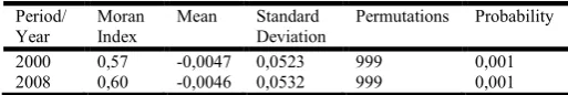
[image:5.595.303.560.195.238.2]Where z i and z j are standardized variables and the sum over j is such that only the value of j∈J in eighbors are included. The J is et covers the neighbors ofiobservation. Table 2showsthe results for statistical univariate local spatialassociationof the Moran indexfor the dependentvariableis the annualgrowth rate offorest clearing. The results indicate thattheMoranindices of0.57 (2000), and 0.60(2008) shows a positivelocal spatial self-correction, in 2000and 2008.
Table 2. Moran Index Statistics for annual growth rate of forest clearing-Space Auto Correct Test Local Univariate-LISA
Period/ Year
Moran Index
Mean Standard Deviation
Permutations Probability 2000 0,57 -0,0047 0,0523 999 0,001 2008 0,60 -0,0046 0,0532 999 0,001
Source: own elaboration. Note: the pseudo-empirical significance based on 999 random permutations.
The LISA statistic provides clear indication that the deforestation rate of growth is extremely auto correlated locally in space through different cities of Pará. Note that the presence of agglomeration regions or spatial clusters of growth or stagnation of deforestation was confirmed by the results provided by the instrumental of local spatial association. According to Vieira, (2009, p. 67):
The LISA methodology allows a local analysis of the spatial pattern of the data, and takes into account the spatial influencein certain regions, while other regions do not show statistically significant groupings. For the full detail of the results, it is necessary to draw an analysis from the scatter diagram showing the spatial lag of the variable of interest, ie the weighted average of the attributein the neighboring municipalities belonging to the vertical axis, and the value of variable of interest on the horizontal axis of the map spatial clusters. For more significant results, it is important to complement the analysis by extracting the results from the spatialcluster map.
high-high type in the municipalities that are part of the Lower Amazon or western Pará, represented by the color legend red, encompassinga total of 15municipalitiesPará. Are they: Santarém, Aveiro, Uruará, Placas, Rurópolis, Itaituba, Jacareacanga, Novo Progresso, Altamira, Brasil Novo, Curuá, Medicilândia, Porto de Moz, Prainha, Trairão. This same type of situation happened in the districts of South and Southeast of Pará, jumping to a total of 40municipalities with positive local
[image:6.595.47.562.46.218.2]spatial auto correlation, with presence of spatialcluster, suchas: São Félix do Xingu, Anapu, Bannach, Pacajá, Novo Repartimento, Itupiranga, Nova Ipixuna, Jacundá, Marabá, Parauapebas, Canaã dos Carajás, Curionópolis, Água Azul do Norte, Tucumã, Ourilândia do Norte, Cumaru do Norte, Santana do Araguaia, Santa Maria das Barreiras, Redenção, Conceição do Araguaia, Floresta do Araguaia, Rio Maria, Xinguara, Sapucaia, Curionópolis, Eldorado dos Carajás, São
Figure 1 a. Cluster LISAMap to Forest Deforestation ratein 2000. Source: own elaboration.
[image:6.595.124.479.283.694.2]Figure 1b. Cluster LISA Map to Forest Deforestation rate in 2008. Source: own elaboration
Table 2a. Classic Model OLS-Growth Forest Deforestation in Paráin 2000.
SummaryofRegression Equation 1 Equation 2 Equation 3 Equation 4 Number of Observations: 143
LNDEF00 Constant
1,7970 -0,2268 -0,8888 -2,1893
P-value (0,0000) (0,7645) (0,2382) (0,0061)
LNbovin00 0,4951 0,4752 0,4136 0,3298
P-value (0,0000) (0,0000) (0,0000) (0,0000)
LNGDP00 - 0,2092 0,1419 0,2094
P-value - (0,0023) (0,03748) (0,0000)
LNRuralCredit00 - - 0,1587 0,1310
P-value - - (0,0005) (0,0030)
LNDistan00 - - - 0,3077
P-value - - - (0,0001)
LNEnvManb00 - - - -0,0007
P-value - - - (0,0673)
Adjusted R²
- - 0,5356
- - 0,5654
- - 0,6012
- - 0,6413
F statistic 162,631 91,1023 69,8661 61,687
Log Likelihood -191,58 -186,826 -180,684 -173,113
AIC (Akaike Information Criterion) 387,16 379,651 369,367 356,225 SC (Schwarz Criterion) 393,085 388,54 381,219 371,04 Diagnosis of Regression
Multicollinearity (MCN) 10,0113 23,0060 26,5621 32,5730
Jarque-Bera (JB) 93,9275 103,177 90,1754 55,9290
P-value (0,0000) (0,0000) (0,0000) (0,0000)
Diagnostic Heteroskedasticity
Breusch-Pagan Test 0,0874 0,7988 15,6580 25,1572
P-value (0,7674) (0,6706) (0,0013) (0,0000)
Koenker-Bassett Test 0,0353 0,3149 6,2807 11,6927
P-value (0,8507) (0,8542) (0,0987) (0,0000)
White test (Robustness) 0,2180 3,4531 10,5853 27,4608
P-value (0,8967) (0,6304) (0,3052) (0,0167)
Space Dependence Diagnosis
Moran`I (error) 4,5236 4,4518 3,6723 3,8389
Valor-z (0,0000) (0,0000) (0,0002) (0,0001)
Lagrange Multiplier (lag) 33,0104 33,7026 27,9191 17,9679
P-value (0,0000) (0,0000) (0,0000) (0,0000)
Robust LM (lag) 15,5549 17,0443 17,3124 7,0760
P-value (0,0000) (0,0000) (0,0000) (0,0078)
LagrangeMultiplier (error) 17,4581 16,6583 10,7784 11,0849
P-value (0,0000) (0,0000) (0,0010) (0,0008)
Robust LM (error) 0,0026 0,0000 0,1717 0,1930
P-value (0,9591) (0,9966) (0,6785) (06603)
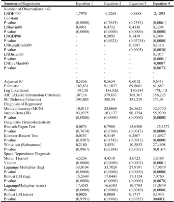
Geraldo do Araguaia, Brejo Grande do Araguaia, São Domingos do Araguaia, São João do Araguaia, Bom Jesus do Tocantins, Jacundá, Rondon do Pará, Don Eliseu, Ulianópolis, Piçarra, Baião, Breu Branco, Goianésia do Pará. Therefore, the resultsfor the year2008of the high-high ratio show that the municipalities forming the western Pará and the south southeast Pará continue concentrating the highest rates of forest clearing, and have adjacent neighbors that they have high rates deforestation, too, cangive this result to the degree of influence that the proximities between regions exercise some envelopes other, confirming the hypothesis that the cities with the highest forest deforestation rates influence neighboring regions due to spatial proximity, also in the period of 2008. The use of explanatory variables with values of the initial period, both for the year2000 and for the year 2008 were necessary to control the endogeneity. After identifying the presence of spatial autocorrelation, through various tests obtained by the Moran index, you must now identify the most appropriate econometric model. Thus, the spatial weight matrix used for the formation of spatial econometric model selected, among several tested is the type Queen because it considers two neighboring regions with common borders. The Table 2(a) and Table 2(b) show the results of the classica lOLS econometric model and the testing of Lagrange multipliers (Lagrange multiplier), and the results of the reasons likelihood (log likelihood) for identifying type sautocorrelation, so we test the null hypothesis ρ=0 and λ=0.
[image:7.595.109.487.74.458.2]If there is rejection of the nullhypothesis in the econometric model with spatial lag, this indicates that the OLS estimators are biased and inefficient, but if there is a rejection of the null hypothesis in the model with spatial error or spatial error, there is no biasor inconsistency, but are not efficient. There gression results obtained via the two OLS for the time periods analyzed showed a coefficient of determination, that is, set R2 with a significant statistical increase of43.37% (Equation 1) to49.57% (Equation 4) in 2000; and62.09% (Equation 1) to71.40%in 2008. Statistical values obtained by the explanatory variables, all transformed into logarithm of neperianbase, such as effective of cattle; gross domestic product (GDP); ruralcredit for cattle ranching; and the shipping cost from the Districtto the nearest capital (distance). The results of the two analysis periods indicate that all input variables were statistically significant with a value-ρ below 5% probability, which indicates the stability of the coefficients of there gressionestimates over, with a clear indication of most statistical robust ness. The results obtained by means of Breusch Paganand Koenker-Bassetttests indicate the absence of heteroscedastic errors. The White test found the lack of poor specification of the various regressions were run. Another important evaluation criterion concerns the Akaike Information Criterion (AIC) and the Schwartz Criterion (SC). The AIC is a F statistic requentemente used for choosing the optimal specification of aregression equation for nonnested alternatives, so when you want to decide between two
Table 2b. Classic Model OLS-Growth Forest Deforestation in Paráin 2008
SummaryofRegression Equation 1 Equation 2 Equation 3 Equation 4 Number of Observations: 143
LNDEF08 (Dependent Variable)
Constant 1,5707 -0,9166 -1,9114 -2,8042
P-value (0,0000) (0,1843) (0,0061) (0,0031)
LNbovin08 0,4991 0,4796 0,3517 0,3186
P-value (0,0000) (0,0000) (0,0000) (0,0000)
LNGDP08 - 0,2296 0,2000 0,2253
P-value - (0,0076) (0,0000) (0,0000)
LNRuralCredit08 - - 0,2021 0,1780
P-value - - (0,0000) (0,0003)
LNDistan08 - - - 0,1586
P-value - - - (0,0366)
LNEnvManb08 - - - -0,0031
P-value - - - (0,7833)
Adjusted R²
- - 0,6209
- - 0,6593
- - 0,7040
- - 0,7140
F statistic 233,609 138,438 110,243 56,6043
Log Likelihood -176,56 -168,407 -140,26 -156,908
AIC (Akaike Information Criterion) 357,12 342,814 326,719 327,816
SC (Schwarz Criterion) 363,045 351,703 338,571 348,555
Diagnostic Heteroskedasticity
Breusch-Pagan Test 1,5986 4,0728 9,2521 19,7069
P-value (0,2060) (0,1304) (0,02611) (0,0031)
Koenker-Bassett Test 0,6314 1,5785 3,6288 8,5599
P-value (0,4268) (0,4541) (0,3044) (0,1998)
White test (Robustness) 2,1032 2,4962 8,5134 38,2831
P-value (0,3493) (0,7770) (0,4833) (0,0734)
Space Dependence Diagnosis
Moran I (error) 0,1369 0,1128 0,1310 0,1374
Lagrange Multiplier (lag) 17,2535 15,3358 11,8728 8,4175
P-value (0,0000) (0,0000) (0,0000) (0,0037)
Robust LM (lag) 10,8472 11,1645 5,9466 2,4730
P-value (0,0000) (0,0000) (0,0147) (0,1158)
LagrangeMultiplier (error) 6,6395 4,5065 6,0822 6,6924
P-value (0,0099) (0,0337) (0,0136) (0,0096)
Robust LM (error) 0,2332 0,3352 0,1560 0,7479
P-value (0,6290) (0,5626) (0,6928) (0,3871)
modelsnot nested, the bestis what produces the lowest AIC value. But the SCis a statisticsimilar to AIC with the feature to imposea higher penalty for the inclusion of additional coefficients to be estimated. In all models tested, the best choice of moread justed econometric model was that of Equation 3for the year 2000 and 2008. Furthermore, statistical test so btained from the Lagrange multipliers- ML(Lagrange Multiplier-LM), MLlag and MLerror reject the nullhypothesis of nospatial autocorrelation, as both the MLLagas MLErrorare statistically significant and positivein all the equations of the econometric model, via OLS, but, asin comparative terms the MLLag Robustis more significant in relation to Robust MLError, in all the equations, with a P-value ofbelow 0.001.
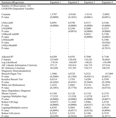
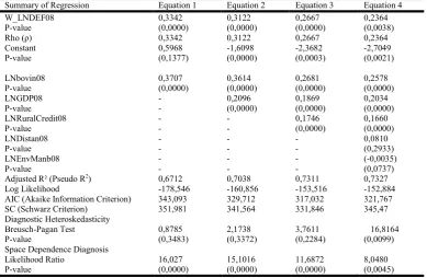
[image:8.595.113.468.70.325.2]Thus, the idealchoice isestimation of the parameters of the econometricspatial model forspatial lagmethod. After completing the diagnosis that suggested the choice of the spatial lag model (spatial lag) as the most appropriate, the results obtained by maximum likelihood estimation of the model with spatial lag in the four equations are presented, and all four models worked showed a great degree of adjustment of the theoretical model. The value-ρ had a positive and significant sign in the two models estimated for both 2000 and 2008, implying that the forest clearing in certain municipalities in Pará involves a direct spatial relationship with the practice of deforestation in a neighboring municipality. Adjustments measures (adhesions) of MV models are: Log-Likelihood (LL), AIC and SC.
Table 3a. Maximum Likelihood Model with Spatial Lag (Spatial Lag)-Growth Forest Deforestation in Paráin 2000
SummaryofRegression Equation 1 Equation 2 Equation 3 Equation 4 W_LNDEF00
P-value Rho (ρ) Constant
0,4768 (0,0000) 0,4768 -1,3443
0,4739 (0,0000) 0,4739 -3,9833
0,4537 (0,0000) 0,4537 -4,2958
0,4283 (0,0000) 0,4283 -5,7824
P-value (0,0330) (0,0000) (0,0001) (0,0000)
LNbovin00 0,4531 0,4283 0,4021 0,3688
P-value (0,0000) (0,0000) (0,0000) (0,0000)
LNGDP00 - 0,2736 0,2374 0,2550
Valor-0070 - (0,0047) (0,0179) (0,0201)
LNRuralCredit00 - - 0,0864 0,0815
P-value - - (0,1997) (0,2287)
LNDistan00 - - - 0,1310
P-value - - - (0,3299)
LNEnvManb00 - - - (-0,0080)
P-value
Adjusted R²(Pseudo R2)
- 0,5121
- 0,5378
- 0,5421
(0,0070) 0,5490
Log Likelihood -245,349 -241,453 -240,636 -239,378
AIC (Akaike Information Criterion) 296,697 290,905 291,273 294,755 SC (Schwarz Criterion) 305,586 302,757 306,087 318,458 Diagnostic Heteroskedasticity
Breusch-Pagan Test 4,0950 11,1531 16,5178 53,7362
P-value (0,0430) (0,0037) (0,0008) (0,0000)
Space Dependence Diagnosis
Likelihood Ratio 17,0525 17,5436 15,8740 13,4172
P-value (0,0000) (0,0000) (0,0000) (0,0000)
Source: ownelaboration.
Table 3b. Maximum Likelihood Model with Spatial Lag (Spatial Lag)-Growth Forest Deforestationin Paráin 2008
Summary of Regression Equation 1 Equation 2 Equation 3 Equation 4 W_LNDEF08
P-value Rho (ρ) Constant
0,3342 (0,0000) 0,3342 0,5968
0,3122 (0,0000) 0,3122 -1,6098
0,2667 (0,0000) 0,2667 -2,3682
0,2364 (0,0038) 0,2364 -2,7049
P-value (0,1377) (0,0000) (0,0003) (0,0021)
LNbovin08 0,3707 0,3614 0,2681 0,2578
P-value (0,0000) (0,0000) (0,0000) (0,0000)
LNGDP08 - 0,2096 0,1869 0,2034
P-value - (0,0000) (0,0000) (0,0000)
LNRuralCredit08 - - 0,1746 0,1660
P-value - - (0,0000) (0,0000)
LNDistan08 - - - 0,0810
P-value - - - (0,2933)
LNEnvManb08 - - - (-0,0035)
P-value - - - (0,0737)
Adjusted R² (Pseudo R2)
Log Likelihood
0,6712 -178,546
0,7038 -160,856
0,7311 -153,516
0,7327 -152,884 AIC (Akaike Information Criterion) 343,093 329,712 317,032 321,767
SC (Schwarz Criterion) 351,981 341,564 331,846 345,47
Diagnostic Heteroskedasticity
Breusch-Pagan Test 0,8785 2,1738 3,7611 16,8164
P-value (0,3483) (0,3372) (0,2284) (0,0099)
Space Dependence Diagnosis
Likelihood Ratio 16,027 15,1016 11,6872 8,0480
P-value (0,0000) (0,0000) (0,0000) (0,0045)
[image:8.595.98.488.368.622.2]It is noteworthy that decision rule is very clear, after all, the higher the value of the LL and the lower the values of AIC and SC, the better the model to capture the spatial relationship of dependency of the variables analyzed. From Table 3 (a) and 3 (b), it is possible to identify the high quality of fit of this regression obtained by the largest value assumed maximum likelihood function (LL) the spatial lag model relative to OLS for the two periods, 2000 and 2008. In relation to AIC and SC, the most significant results for the year 2000 and 2008 are found in the MV model with spatial lag. Analysis of the spatial autoregressive model in the variable shows that there is no evidence of heteroskedasticity in the residuals at a level of 5% as seen by the BP test. For the results shown in Table3 (a) and 3 (b), there is no evidence of remaining spatial autocorrelation in the waste, which indicates that the spatialgap in the dependent variable has been properly modeled. It should be noted also thatthe value of the spatial lag regression coefficient, represented by ρ(rho), proved to be statistically significantwith a value of 0.4768(2000) and0.3342(2008), indicating that the modelspatial lagis extremely suitable to treat the spatial dependence. It isa word of caution: it is tempting to focus on the traditional measures of conventional regressions, as theR², to confer the degree of fitof an econometrictime series model. However, this procedureis not appropriatein adata modelincross-sectionn on-space. In fact, the value of R²Adjustedspatiallagmodel is not therealvalue ofR²but aPseudo-R², which cannot be directlycompared with the value ofrealR²ofOLS, this because thePseudo-R² isratio of the variance of the predicted values andthe variance of the observed values. With regard to the variables used in the spatial lag model, estimated by Maximum Likelihood, maintained apositive patternand significance with value-ρbelow 5% probability, that is, the growth of forest clearinginthe State of Parámunicipalities involves some kind of spatialexternality. This means that the growth of forest clearingin a givenmunicipality Paradepends on the deforestation of its neighbors growth, which may show the presence ofpositive externalities(or negative) that influence the increase (ordecrease) of forest deforestation rate of any ounty Pará State. The explanatory variables are variables that directly influence, orthathypothetically help explainthe dependent variable. Thus, with the focus of analysisin Table3 (a)and Table3(b), inunder standing the explanatory variables, which were the object of research of the econometric modelofspatial lag, have yielded the following conclusions. Are they:
I) Effectivebovinecattle: the coefficient of this explanatory variable, which was spatiallylagged, showed a positivesignalin two models: OLS, MV with spatial lag, bothfrom 2000and for theyear 2008.At each incrementthe effectiveofcattlein Pará,mainlyin the districts ofWest, South andSoutheast, siteswith the highestnumber ofcattlein the region, have adirect influencerelationship with forest deforestation rates in neighboringmunicipalities, ie, model results show that the pattern of forest clearingin Para incorporates the effects of space overflow. In general, the cattle herdisa valuedandactiveat the same time, when transformed intofreshor processedmeat, a health food consumption in great demandindomestic and international markets, which contributes to both the price of bare groundasthesize of the cattle herdfavor the expansion of livestock threshold into the areas ofdense forests, causing deforestation. From the point of view ofcapital, thecattle herdis a commodity with the power to ensure ownership of the land, a fact of great importance in a borderregion likePará.
Evenin an extremelywide territory, the issue of logisticsinvo lving handling andtransportation of livestockis notan apparent problem forthe farmer, especially when using opportunistic mechanisms to circumvent the scrutinywithillegal practices involving corruption of the agents involved init. According to Margulis (2002, p. 15), "the issue of investment in technology andproductivityis another factor that intensive the relationship betweenlivestock and deforestation". He claims that thelocal playersarequickly becoming more professional by virtue of the mselvesincreasingly competitive markets, and thereforethere isan inexorabletrendofintensificationsystems andwidespread increase inproduction efficiency, as a possible explanationfor extensive livestock farmingareearnings perhectarevery low, forcing thelarge-scale production.
The statistical resultsreveala lower-ρvaluethan the significancelevel of 1%, which shows that the resultsof this variableis significantin allthe fourequations.Thus, forevery 1% increase of actual cattlein Pará,in the orderof45.31% in 2000and37.07% in 2008, comes from theneighboring municipalities.
Economic Growth (GDP): the coefficientof this lagged explanatory variablespatially gavepositivesignals in allfour equations, which shows that the increase inGDP of agiven municipalityin Para influenceopenly forestdeforestation ratesin the adjacentmunicipalitiesto it.The results showthat the pattern ofeconomic growth ofParámunicipalitiesinclude the effectsof spatialspillovers, with economic growth of Parámunicipalitiesspreading theforest clearing. Notesthatfarming isthe maineconomic activityof the region,andthe financial viability oflarge andmediumranchersis the sourceof the processof deforestation in BrazilianAmazoniaaccountingcurrently for around75% ofdeforested areasin Amazonia. The relationship between economic growth and deforestation is evident in the socioeconomic indicators of Pará. Despite the rise of socioeconomic indicators, such as per capita income, for example, there are large inequalities in the region, especially regarding the distribution of income and the quality of life of local people. The statistic considers a value-ρ less than the significance level of 1%, showing statistically significant results in all the equations, and for every 1% increase in GDP in the State of Pará, in the order of 27.36% in 2000 and 20.96% in 2008 comes from the neighboring municipalities.
Constitution itself, where the state of Pará was invested from 1999 to 2006 a value of approximately R $ 3.16 billion in rural credit, and of this total, US $ 1 billion was earmarked for agriculture and R $ 2.15 billion for livestock. So through the spatial econometric instrumental was possible to buy the volume of rural credit is related to the rate of loss of forest cover, creating somehow spillovers effects of rural credit to urban areas of Pará State. The value-ρ presented value less than the 5% significance level in all the equations, and for each 1% increase rural credit granted to the State of Pará municipalities in the order of 8.64% in 2000 and 17.46% in 2008 , come from the municipalities close to each other.
Expenses on Environmental Management
The coefficient of this explanatory variable, which indicates the existence of spending onlabor, work, funding and equipment, in short, a factor that expresses the capacity of action of environmentalinstitutionsto combat deforestation, has laggedspatiallyand provided negative signin both periods:-0.0081(2000) and-0.0035(2008).This demonstratesthat there wasa decrease inforest clearing. Government spending in Environmental Managementconsist of the federal governmentachievementswhosegoal is to preservethe natural stateof a givenareain the municipalityorits recoverywhensome environmentaldamage isfocused onthis area. These expenses are, in financial terms, theless expressive. Although the government hasseveral programsrelated to the environment, analysis of their spendingshows that his actionsstill needmore resources, especially inan extremelyextensiveterritorial State. The factor that involves spending on environmental management is statistically significant, and its signal is supported by the basic assumptions of the model. Therefore, the larger the expenses on environmental management, the greater the reduction of forest deforestation rate in Pará. It is clear that the amount of spending is still well short of what it should be, but the effectiveness of this action is already clear. In the analysis by the maximum likelihood method with spatial lag, it can be seen that for each 1% of amounts spent on environmental management, there is a reduction of 0.81% of forest clearing in 2000; and 0.35% in 2008.
Roads(costof transport)
This variableis statistically significant, demonstrating that the cost of transportationis one of theinducingvariablesofforest clearingin Paraprimarily in aborder region, as well asfederal, state and local roads, there are also undergroundroads that areopeninsidethe forest, contributing to an extremely aggressiveforest clearing. In addition, there is the problem involving unofficial or illegal road networks as major cause of deforestation, especially those opened by loggers. As Anderson and Reis (1997), the opening of roads and subsidized credit have different impacts on deforestation, as 96,000 km2 of deforested area can be attributed to both, but the roads are responsible for 72%, while the subsidized credit by 28%. In addition, the impact of the opening of roads is much worse than the credit because they cause large deforestation and small increase in production. The result obtained in this variable reveals a lower-ρ value than the significance level of 5%, which shows that the statistical results of this variable are significant statistically, and for each 1% spent on transport costs given the distance, in order of 13.10% comes from neighboring towns and 15.86% in 2000.
In 2008, furthermore, the spatial spillover effect for this variable is extremely significant.
Conclusion
The demographic and economic processes of occupation of the great Amazon frontier were initially articulated by the action of the federal government, at the time of military dictatorship, and dependent on the economic interests of entrepreneurs in the South-Central and cheap and abundant labor, work that migrated from other regions, especially the Northeast. The low population density and lack of basic social capital (economic infrastructure) in the Amazon resulted in relatively low land prices compared to the rest of Brazil. These conditions provided the stimulus for the integration of the Amazon frontier to the rest of the country. This integration in economic terms is given initially by the private ownership of land, often by their own violent processes of primitive accumulation, leading to consolidation of the rights of capitalist property by illegal means followed by the clearing of forests to the occupation of land by agricultural activities. The initial occupation and the expansion of the agricultural frontier (and other economic activities, such as mining), in turn, generate new and more demands for hand labor that with the government propaganda with its directed colonization projects, which attracted new migratory flows causing a spontaneous colonization process.
Plan, becomeswelcomeas theBrazilian economynow hasmorea factor ofeconomicbuoyancy, vigorous, which does not exist inmost countries in theworld economy.On the other hand, the question of the Amazon rainforestzdeforestationzbecomes thenewshowcase the actions ofnon-governmental organizations and the media in general. Little attention was giventothe Amazon andto Pará, despitelocalizedpolicycreation of extractive reserves, resulting in a significant increase in forest deforestation. In the government of President Lula, the Ministry of Environment (MMA) opened a front to combat illegal logging in the Amazon intensifying supervision. This resulted in a significant reduction of forest deforestation rate that led Brazil to be the first country in the world to effect compliance with feasible targets for reducing greenhouse gases. Anyway, what can be concluded is the realization that new institutions created to combat the increase of deforestation of the Amazon and governance mechanisms adopted in national and state policies to combat deforestation of the Amazon rainforest in Para has achieved positive results in the last years old. In addition, the increasedexpansion of cattle ranchingin the Amazondriven by demand from abroadhasdirectly influencedthe increaseof deforestation, hindering thedevelopment of the activityin a sustainable way in the region.In this regard,theexpansion of cattle ranchingin the Amazonover the past decadeisalso relatedto the dynamicsof the domestic marketof resources and land, directing, mainly, to Pará. In the case ofbeef productioninParáregion, there is an ongoingverticalization processof agribusinesswith the presence ofrefrigerators andtanneriesand other derivatives. Clearly, too, the advance ofsoybean productionand newsub-regional economic centersin Pará,being createdfrom the discoveryof new sources ofmineral resources.Finally, we highlight the importance ofspatialeconometricinstrumentalasextremely usefultoolto perform variousresearch involvingempirical testsontheoretical assumptionsor comparisonswiththe results presented bystandardeconometrics, especially when itmakes useof the particularitiesof this area which involvesspatialself-correctionandspatial dependence.
REFERENCES
ANDERSEN, L.E. GRANGER, C.W.J., REIS, E.J.1997. A randon coefficient VAR transition tidamodel of the changes in land use in the Brazilian Amazon. Revista de Econometria, v.17, n.1.
ANSELIN, Luc (1988). Spatial Econometrics: Methods and Models. Dordrecht, Kluwer Academic Publishers. ANSELIN, L. (1995). “Local indicators of spatial association
– LISA”, Geographical Analysis. V 27 (2), April. p. 93-115.
ANSELIN, Luc. (2005). Exploring Spatial Data with GeoDa – A Workbook Spatial Analysis Laboratory, Department of Geography University of Ilinois, Urban-Champaign, Urban, IL 61801 and Centre for Spatially Integrated Social Science.
ANSELIN, Luc and BERA, A.K. (1998) Spatial dependence in linear regression models with an introduction to spatial econometrics.Handbook of applied economic statistics (ed. by A. Ullah and D.E.A. Giles), pp. 237–289. Marcel Dekker, New York.
ANSELIN, LUC and LOZANO-GRACIA, Nancy. (2008). "Errors in variables and spatial effects in hedonic house price models of ambient air quality," Empirical Economics, Springer, vol. 34(1), pages 5-34, February. CHIARINI, Tulio. (2009) Acesso a serviços públicos e
pobreza no Rio Grande do Sul: uma análise espacial – 2000. Ensaios FEE, Porto Alegre, v. 30, n.1, p. 195 – 228. FEARNSIDE, Philip M. (2003). A Floresta Amazônica nas
Mudanças Globais. Manaus, INPA.
FERRAZ, C. (2001). Explaining agriculture expansion and deforestation: evidence from the Braziliam Amazon-1980-1998. Texto para Discussão, Nº 828. Brasília, IPEA/DIPES.
FLORAX, R. J. G. M., FOLMER, H., REY, S. J. (2003). “Specification searches in spatial econometrics: The relevance of Hendry´s methodology”, Regional Science and Urban Economics, vol. 33, n. 5, p. 557-79.
GARCIA, R.A., SOARES-FILHO B.S., MORO, S., 2004. Modelagem espacial do desmatamento amazônico. XIV Encontro Nacional de Estudos Populacionais, ABEP. Anais. Caxambu, Brasil.
IGLIORI, D. (2008). Deforestation, growth and agglomeration effects: evidence from agriculture in the Brazilian Amazon. Discussion paper series: University of Cambridge, department of land economy, nº 28. UK.. MARGULIS, S. (2002). Quem são os agentes dos
desmatamentos na Amazônia e por que eles desmatam?Word Bank internal paper.
MORAN, E. (1996). “Deforestation in the Brazilian Amazon”. In: SPONZEL, L.E. et al.(Ed.). Tropical deforestation: the human dimension. NY, Columbia University Press. PAELINCK, Jean H.P (2005). Spatial econometrics: history
state-of-the-art and challenges ahead. WORKSHOP ON SPATIAL ECONOMETRICS.Kiel:Institute for World Economics.
REYDON, Bastiaan Philip & PLATA, Ludwig (2000). “Políticas de mercado de tierras en Brasil”, PolíticasAgrícolas, Volume Especial. Santa Fé de Bogotá, Colômbia.
VIEIRA, Rodrigo de Souza. (2009). Crescimento econômico no Estado de São Paulo: uma análise espacial. Ed. Cultura Acadêmica.