Munich Personal RePEc Archive
Status, fertility, growth and the great
transition
Tournemaine, Frederic and Tsoukis, Christopher
University of the Thai Chamber of Commerce, London Metropolitan
University
8 February 2008
Status, fertility, growth and the great transition
∗
Frederic Tournemaine
†School of Economics, University of Chicago-UTCC Research Center
University of the Thai Chamber of Commerce
126/1 Vibhavadee-Rangsit Road, Dindaeng, Bangkok, 10400, Thailand.
Christopher Tsoukis
Department of Economics, London Metropolitan University
84 Moorgate, London EC2M 6SQ, UK.
February, 2008
Abstract
We develop an overlapping generation model to examine how the relationship between status concerns, fertility and education affect growth performances. Re-sults are threefold. First, we show that stronger status motives heighten the desire
of parents to have fewer but better educated children, which may foster economic
development. Second, government should sometimes postpone the introduction of
an economic policy in order to maintain the process of economic development,
al-though such a policy aims to implement the social optimum. Third, status can
alter the dynamic path of the economy and help to explain the facts about fertility
during the “great transition”.
JEL Classification: D31, O41.
Keywords: social status, fertility, education, economic policy.
∗We would like to thank the seminar participants at the Singapore Economic Review Conference in
August 2008 for useful comments and suggestions.
1
Introduction
The idea that individuals derive utility not only from their level of consumption but also
from their relative position in society is by now well established. Also nicknamed “keeping
up with the Joneses”, this concept has been used to explain the equity premium puzzle
in finance (Abel, 1990), to raise issues about taxation (Ljungqvist and Uhlig, 2000) and competition (Dixon, 2000). In growth models, it has been used to analyze the impact of
social relations on growth performance (Corneo and Jeanne, 1997; Fershtman, Murphy
and Weiss, 1996; Futagami and Shibata, 1998; Pham, 2005; Tournemaine and Tsoukis,
2008).
In this paper, we investigate how such status considerations can alter individuals’
decisions to bring up and educate children. This issue is important for two reasons. First,
there seems to be a trade-off between the expectation to achieve a position in society and the desire to bring up children (Tournemaine, 2008). Recent empirical studies have
shown a parallel increase in women’s level of education and participation into the labor
force at the same time as a decrease in fertility rates (see Black and Juhn, 2000; Dolado,
Felgueroso and Jimeno, 2001 and 2002; Sheran, 2007). In this paper, we then attempt to
give a possible explanation to the upstream factor inducing such behavior. We argue that
the decision to have children can be seen as a threat to achieving any career and obtain
one’s place in society. This notion parallels that of Becker (1991) who pointed out that
bringing up children into adulthood is costly, especially in terms of the mother’s time
because women are the primary providers of child care.
Second, the link between quality (education) and quantity of children has been
recog-nized for many years in the literature. It is now well admitted that economic development
goes along with a general decline in fertility rates and an increase in investment in
ed-ucation (Galor and Weil, 1999; Doepke, 2004). The existence of a trade-off regarding the parents’ decisions between the quality and quantity of children is often considered
as a factor which has contributed to the transition of economies from a stage of
stagna-tion (poverty trap) to perpetual growth (Becker, Murphy and Tamura, 1990; hereafter
trade-offbetween quality and quantity of children. More precisely, if seeking greater so-cial status induces parents to increase their investment in the education of their children,
social status is a factor which can perhaps help to explain why countries have left the
poverty trap in which they seemed to be stuck and initiated a “great transition” to a state
of development.1
Galor and Weil (1999) argue that the process of economic development can be divided
in three main stages: a Malthusian regime, characterized by stagnation and
underdevelop-ment where fertility and mortality are high; then, a Post Malthusian Regime where there
is an acceleration of technological progress and an increase in per capita income
accompa-nied by a declinefirst in mortality, and a rise, then a fall in the fertility rate; andfinally, a modern regime where incomes per capita is high and fertility and mortality rates are low.
Thus, in a plot of net fertility (i.e., the population growth rate) against growth, or the
stage of development, the data appears to show an inverted U-shaped curve (see Galor,
2005; and Section 4 for the case of some Asian countries). Accounting for this evidence
seems a challenge for BMT, as their analysis implies only a drop of fertility across the
two regimes. However, reconsidering the BMT framework enhanced to account for social
status, we show that the transitional dynamics can replicate such empirical evidence.
Moreover, we show that introducing social aspirations in the basic BMT framework
has important policy implications. In order to eliminate the distortion arising from the
consumption externality (“keeping up with the Joneses”) and implement the optimum,
a major conclusion of the relevant literature is that government intervention by means
of a tax on consumption is desirable. In contrast, the interesting result here is that the
policy-maker should sometimes postpone the introduction of such a policy in order to
maintain a long-run self-sustaining economic growth. The idea that an economic policy is
1While the broad outlines of the Industrial Revolution and the ”great transition” are known, by no
not desirable and might be postponed is well known in other fields of economics such as trade and finance.2 However, to our knowledge, this notion has not been raised in a
the-oretical growth model, although some authors have investigated the relationship between
trade liberalisation and growth. For instance, empirical findings of Greenaway, Morgan and Wright (2002) suggest that trade liberalization has resulted in both an increase and
decrease in the growth rate depending on country circumstances. In this paper, the
ar-gument in favour of (or against) the postponement of the consumption-tax policy is that
this tax reduces the return to investment in children’s education. That is, it gives
in-centives to parents to replace quality of children with more quantity; as a result, parents
could stop investing in education. Thus, although the policy aims to maximize welfare,
it could also break the process of economic development and the country could end up
in a poverty trap. In order to avoid this situation, the government should implement the
social optimum only when the return to investment in education is sufficiently high to maintain incentives to educate children even after the introduction of the tax.
Thus, our contribution is summarised as follows: We introduce status considerations
in the BMT framework, and investigate how they alter individuals’ decisions to bring up
and educate children, ceteris paribus we examine how they affect growth and develop-ment. It is worthwhile to note here that in comparison with the basic literature focusing
on growth and social status, we give an alternative approach to the growth process by
placing both human capital and fertility at the centre of the analysis. We also derive
pol-icy implications, particularly the desirability of postponing the otherwise optimal polpol-icy
of offsetting consumption externalities by taxation. We finally develop the transitional dynamics of the model, hitherto ignored, and show that our framework can replicate the
empirical observation that there is an inverted U-shaped relationship between fertility
and development.
The remainder of the paper is organized as follows. In Section 2, we present the model.
2For example, since the early 90’s, the “Washington Consensus” has largely influenced the policy
In Section 3, we examine its key properties regarding the status motives of individuals,
fertility, education and growth. The transitional dynamics is developed in Section 4. We
conclude in Section 5.
2
Model
The main building block of the model is taken from BMT. Time, denoted byt, is discrete
and goes from 0 to ∞. The economy is populated by overlapping generations of people
who live for two periods: childhood and adulthood. All decisions are made in the adult
period of life. Each adult individual is endowed with one unit of labor that she supplies
inelastically between the production of a consumption good and raising children to
adult-hood. Parents and children are linked through altruism, i.e. parents care about their own
welfare but also that of each of their children. Following Rauscher (1997), Fisher and Hof
(2000), Tsoukis (2007), the social status of adult individuals is measured by the ratio of
their level of consumption,ct,to the average level of consumption of all other individuals,
ct,which is taken as given. Formally, preferences of an adult individual at timetare given
by
Vt=
[(ct)Ψ(ct/ct)γ]1−σ
1−σ +α(nt)
1−ε
Vt+1, (1)
whereγ >0,0< σ <1, 0< α <1,0< ε <1, nt is the number of children that a parent
has,Vt+1 is the level of utility that a child will attain as an adult andΨ(ct/ct),whereΨ(·)
is strictly increasing, represents the preference regarding social status. The parametersε
and α are respectively the elasticity of altruism with respect to the number of children
and the degree of altruism of parents toward children.
Observe that the standard preferences (e.g. Barro and Becker 1988, 1989) correspond
to the case of γ = 0 whereby individuals do not derive utility from their social status.
When γ > 0, the utility of an adult individual exhibits a consumption externality: the
“keeping up with the Joneses”. That is, the average level of consumption of people has a
negative effect on the level of utility of an individual. It will be useful to keep this feature in mind when we will study the properties of the model.
A second remark is that the restriction on the value of σ to the range (0,1) is not
as-sume values higher than 1 because this is the case which is empirically supported (see
Hall, 1988). As explained by Ehrlich and Lui (1997) this is “because in the generational
frameworks σ denotes the inverse of the elasticity of substitution in consumption across
consecutive generations, rather than years. Thus, if a generation spans 25 calendar years,
a value ofσ less than 1 could be equivalent to a value substantially above 1 in these other
models” (see footnote 8, pp. 229).
Finally let us mention that there exists other definitions of social status. For instance, Corneo and Jeanne (1997), Futagami and Shibata (1998), Long and Shimomura (2004),
Pham (2005), define it as the level of wealth relative to that of others. This would suggest introducing physical capital accumulation in the model. Adding this variable
would complicate, but not “wash away”, the effects we are discussing here. Similarly, like Fershtman, Murphy and Weiss (1996), we could define social status as the relative level of human capital of individuals. Such a specification would not affect the qualitative results of the paper either.
Raising a child is costly. We assume that it takes a fixed amount of consumption good, f, and a fixed amount of time v to bring up one child to adulthood, where f > 0
and v > 0. Moreover, parents can use an extra amount of their time, et > 0, to teach
each child. The level of human capital of children depends on the level of human capital
of their teachers-parents and on the amount of time their parents spend to teach. The
technology of human capital is
Ht+1=φetHt+H0, (2)
whereφ >0is a productivity parameter andH0 is the innate level of skills of an individual:
if individuals do not invest in education (et= 0), the level of skills of individuals is given
byH0.3
Assuming a linear technology for the production of the consumption good, the resource
constraint is given by
ltHt =ct+fnt, (3)
3We have changed the specification of the human capital technology slightly form that employed by
whereltis the time spent by an adult to the production of the consumption good andfnt
represents the total cost in terms of the consumption good of raisingnt children. Finally,
since people have afixed time endowment equal to unity, the time constraint is
1 =lt+nt(v+et), (4)
where nt(v+et)represents the total cost in time to raise nt children.
3
Equilibrium
3.1
The representative individual’s problem
In this Section, we compute the equilibrium conditions of a representative individual’s
maximization problem. For simplicity, we focus on a symmetric equilibrium, whereby
indi-viduals are identical. The problem of an adult individual consists of choosinglt, et, nt, Ht+1
that maximize (1) subject to (2), (3), (4). After substitution, the problem can be written
as
Vt(Ht) = max nt,Ht+1
1 1−σ
½
Ht
∙ 1−nt
µ
v+ Ht+1−H0
φHt
¶¸ −f nt
¾(1−σ) ×
Ψ
½½
Ht
∙ 1−nt
µ
v+Ht+1−H0
φHt
¶¸ −f nt
¾
/ct
¾γ(1−σ)
+α(nt)1−εVt+1(Ht+1).
Manipulation of the first order condition with respect to nt and using the property of
symmetry (e.g. ct=ct) yields
α(1−ε) (nt)−εVt+1(Ht+1) = [Ht(v+et) +f] [1 +γ∆] (ct)−σ[Ψ(1)]γ(1−σ), (5)
where ∆ ≡ Ψ0(c
t/ct)ct/[Ψ(ct/ct)ct] = Ψ0(1)/Ψ(1) is the elasticity related to the status
effect: ∆ measures how much individuals care about their status. Futagami and Shibata (1998) explain that∆ is the strength of status preference: the greater the value of∆, the
stronger are the status motives of individuals. The left hand side of (5) represents the
children takes time that could alternatively be used to increase the production of the
consumption good which in turn would increase the relative position of the adult-parent
in the society.
Manipulation of the first order condition with respect to Ht+1 yields
(1 +γ∆) (ct)−σ[Ψ(1)]γ(1−σ)≥αφ(nt)−ε
dVt+1
dHt+1
, (6)
where equality holds if et>0. Moreover, the envelope condition implies
dVt+1
dHt+1
= (1−vnt+1) (1 +γ∆) (ct+1)−σ[Ψ(1)]γ(1−σ). (7)
Combining (6) and (7) yields
µ
ct+1
ct
¶σ
≥αφ(nt)−ε(1−vnt+1), (8)
where the left hand side is the marginal rate of substitution between consumption of
parents and children and the right hand side represents the return of investments in
human capital.
3.2
Basic properties
In this sub-section, we analyse how social status affects the choice of fertility and education of individuals and its welfare implication. For simplicity, we restrict our attention to
steady-state equilibria, i.e. we focus on the long-run. The short-run effects of social status are examined in Section 3.3 in which we characterise the transitional dynamics.
3.2.1 Steady-state equilibria
The basic structure of the model combined with the fact that we focus on the symmetric
individuals case implies that three steady-state equilibria can be shown to exist (see
BMT for more details): a stable Malthusian poverty trap, a stable state of persistent and
self-sustaining growth and an unstable intermediate state of development. Proposition 1
summarizes these results, where the symbols “u”,“∗” are used to denote respectively the
value of variables in the Malthusian and self-sustained growth steady-states. A hat, “b”,
For convenience, the following parameter restrictions are assumed throughout the
paper:
Assumption 1:
£
1−v(α/ε)1/(ε−1)¤H
0−f(α/ε)1/(ε−1)
(H0v+f) (1 +γ∆)
< (1−σ)
£
(α/ε)ε/(ε−1)−α(α/ε)1/(ε−1)¤
α(1−ε) .
Assumption 2:
1−ε−(1−σ) (1 +γ∆)>0.
Assumption 1 guarantees the uniqueness of the solution for the equilibrium fertility
rate in the Malthusian steady-state. Assumption 2 guarantees the existence of a growing
steady-state where the amount of time allocated to teaching activities is strictly positive.
Proposition 1 In the Malthusian steady-state, parents do not invest in education of their
children (e.g. eu = 0) which leads to zero economic growth. Under Assumption 1, the
number of children they bring up, nu, is unique. It is the solution of
(1−vnu)H0−fnu
(H0v+f) (1 +γ∆)
= (1−σ) [(nu)
ε
−αnu]
α(1−ε) , (9)
and verifies
(nu)ε> αφ[1−vnu]. (10)
In the growing steady-state, individuals choose to bring up a number of children, n∗,which
is the solution of ∙
vφ(1−σ) (1 +γ∆) 1−ε−(1−σ) (1 +γ∆)
¸σ
=αφ(n∗)−ε(1−vn∗). (11)
The amount of time they allocate to teaching activities, e∗, is given by
e∗ = v(1−σ) (1 +γ∆)
1−ε−(1−σ) (1 +γ∆). (12)
The common growth rate of consumption and human capital, g∗, is given by
g∗ =φe∗−1. (13)
In the intermediate state of development, the fertility rate is the solution of
The human capital of an individual, H,b is constant over time which implies an economic
growth rate equal to zero. It is given by
[1−nb(v+be)]Hb −fbn
b
H+ (v+be) +f =
(1−σ) [(bn)ε−αbn]
α(1−ε) . (15)
where investment in education, be, is given by
b
e= Hb −H0
φHb . (16)
Proof. See Appendix.
A Malthusian steady state is a corner solution: e = 0. It arises because the rate of
return to investment in the quality of children (human capital) is too low relative to the
return to investments in the quantity of children. The return from investing in children
is given by the left hand side of (9). If such a steady-state occurs, it is stable. The reason
is that the condition (10) holds with a strict inequality. Thus, even if the level of human
capital becomes strictly positive, for sufficiently low values ofHt this does not reverse the
inequality. Consequently, the economy will return to the steady-state where Ht =H0 in
all periods. When the level of human capital is sufficiently high, however, the returns to investment in human capital are large enough to break the corner solution (see equation
(8)): the quantity-quality trade-offturns out towards children quality instead of quantity. This is the force that puts the economy on a convergent path to the steady state with
positive growth.
Between the Malthusian and self sustained growth steady-states, an intermediate state
of development can emerge. This steady-state is however unstable. If the initial level of
human capital is higher than the threshold levelH, individualsb find it profitable to invest in education and the economy will keep on growing. On the other hand, if the initial
level of human capital is lower than the threshold level, H, the economy will convergeb
towards the Malthusian steady-state because, in this case, the income effect dominates the substitution one. Figure 1 gives a graphical representation of the above results.
3.2.2 Effects of social aspirations
Proposition 1 allows us to analyze the effects of social aspirations on the choice of fertility and education in each of the three steady-states in which the economy can end up. From
equation (9), the choice of fertility of individuals is negatively correlated with the strength
of social aspirations, ∆. The reason is that higher social aspirations increase the cost of
bringing up additional children (see equation (5)). Thus, adult individuals reduce the
number of children and allocate more time to the production of the consumption good
because they expect to improve their relative position in the society. The outcome is that
condition (10) becomes less restrictive. Thus, as social aspirations increase, a Malthusian
steady state is less likely to occur.
Examination of equations (14), (15), (16) gives a confirmation of this. We can see that stronger status motives reduce the threshold level of human capital required to switch to
the self sustained growth steady-state. Therefore, social status heightens the parents’
decision to substitute quality for quantity of children.
Once the economy is on the self-sustained growth steady-state, stronger social
as-pirations induce a reduction of the fertility rate, n∗, and an increase of investments in
education, e∗. Thus, in turn, stronger status motives foster economic growth, g∗, (see
equations (11), (12), (13)). The reason is that parents take into account that, for their
children, education is the means to increase the production of the consumption good,
thereby their relative position in the society: as generations are linked through altruism,
the success of children in terms of social achievement affects the welfare of parents who prefer to reduce the number of children so as to improve their quality.
Figure 2 gives a graphical representation of the effects of an increase in the strength of social status, ∆, on the three possible steady-states. The plain line, calledC1, represents
the solution of the model. The dotted line, called C2, represents the polar case in which
individuals do not derive utility from social status (e.g. we set γ = 0). Note that C2
represents the socially optimal, benchmark solution of BMT in which social aspirations
do not affect preferences of individuals. In Figure 2, we denote by ³Hb´o the threshold level of human capital of the unstable intermediate state of development in this benchmark
Insert Figure 2 here
It is important to mention that in the perpetual growth regime and in the unstable
intermediate state of development, investments in education are excessive relative to the
situation which is socially optimal (for whichγ = 0). This featurefinds empirical support in the literature (see for instance Kodde and Ritzen, 1984; Oosterbeek and Webbink,
1995). Hence, from the model, we can then argue that preferences for social status are a
possible factor causing these excessive investments.
3.2.3 Social optimum and economic policy
As explained in the previous sub-section, the solution given in Proposition 1 is not socially
optimal because of the presence of the external effect caused by social aspirations. It is thus natural to think about an economic policy which can eliminate this market failure in
order to implement the optimum. To this end, we assume the government’s intervention by
means of a taxτtcharged on the level of consumption of an adult individual. By increasing
the price of consumption, the policy-maker increases the cost at which individuals can
improve their relative position in society. Then, by choosing an appropriate level of tax,
she can obtain an optimal allocation of resources.
For simplicity, we assume that this policy is funded through a lump sum transfer Tt
from individuals and that the budget constraint of the government is balanced at each
moment: Tt=τtct,at all times. Computations lead to the following Proposition:
Proposition 2 If government authorities choose a tax rate, τo, such that
τo =γ∆ at all times,
the equilibrium is optimal.
Proof. See Appendix.
The relevance of this tax is illustrated in Figure 2. The introduction of the economic
policy will induce a downward shift of the curve C1 for which γ >0 to make it coincide
raise at this stage is the following: should the government introduce the economic policy
tool as proposed in Proposition 2? The answer to this question depends on the level of
human capital of individuals when the policy is introduced. From Figure 2, if the level
of human capital of individuals is lower than Hb or greater than (Hb)o, the government
can introduce the economic policy tool in order to reach the optimum; in this case, the
introduction of the tax does not alter the kind of steady-state the economy will end up in
(i.e. Malthusian or self sustained growth). If the human capital of individuals belongs to
the set[H,b (Hb)o],however, the tax will tilt the economy which was developing towards the
Malthusian steady-state poverty trap. Thus, one should wonder whether it is optimal for
a country to choose to become poor. If it is not, government authorities should postpone
the introduction of their economic policy until individuals attain a sufficiently high level of human capital (e.g. slightly greater than (Hb)o) in order to maintain the incentives to
invest in education. In this case, a long-run self-sustaining growth can be maintained and
the optimum can be reached later.
4
Transitional dynamics
In this Section, we study the transitional dynamics of the model; to our knowledge this
has not been done before. As mentioned, this issue is interesting because it allows us
to confront the model to a larger extent to empirical evidence. In particular, as shown
by Galor (2005), there is an inverted U-shaped relationship between net fertility (i.e.
population growth) and income during the transition from the Malthusian steady-state
to the state of perpetual development. We may view the 18th century, with its prolonged
period of stability and processes of ”Smithian growth” as mentioned above, as a ”shock”
that gave an impetus to fertility and growth beyond the threshold derived in the previous
section. Such empirical feature can also be observed for some Asian countries which
displayed good growth performances since the 1960s. Indeed, using annual data from the
IMF (International Financial) over the period 1951-2005, Figure 3 shows the evolution of
the population growth rate in Hong-Kong (HK), Singapore (SI), Malaysia (MA), Thailand
Insert Figure 3 here
We can observe that population growth rate increase before falling down in these
countries: so, countries that exhibited a transition from Malthusian to endogenous growth
regimes showed an inverted U-shaped relationship between population growth and income.
In such context, the aim of this Section is to show that an increase in preferences for
social status can help to explain the above empirical facts. As mortality here is fixed (all individuals live for two periods), our fertility ratent is equivalent to population growth.
To characterise the transitional dynamics we develop a 2×2linearized system in the
amount of time devoted to schooling and human capital around the asymptotic
steady-state of perpetual development. We give a more intuitive exposition here, and relegate
the more formal details to the Appendix. A reminder thatHt, etandntdenote the actual
values of human capital, time devoted to schooling and fertility while Ht∗, e∗, n∗ denote the paths of the variables that would result if the economy were on its steady-state growth
path, growing at a rate g∗ (see Proposition 1). In this Section, deviations, indicated by a
tilde, are the percentage deviations from the path of perpetual development: we denote
e
ht = (Ht − Ht∗)/Ht∗, eet = et − e∗ and net = nt −n∗ these deviations. After tedious
computations described in the Appendix, one gets the following system:
⎡ ⎣ eht+1
e
et+1 ⎤ ⎦=
⎡
⎣ 1 φ/(1 +g∗)
0 χ
⎤ ⎦
⎡ ⎣ eht
e
et
⎤
⎦. (17)
Obviously, there exist a unit root and a stable root χ, where
χ≡ σM−εN/n∗−σφ/(1 +g∗)
Nv(1−vn∗)−1+σM . (18)
It will also be useful below to note during the transition, deviations of the fertility rate
are related to education effort by:
e
nt=Neet, (19)
with
N ≡ −(1−ε)e∗/(v+e∗)
3+ [ε+ (1−ε)n∗e∗]/(v+e∗)2
1 +ε[1−n∗(v+e∗)]/[n∗(v+e∗)] <0.
We assume that the parameters of the model are such that 0 < χ < 1 to ensure
saddle-point stability and avoid oscillatory trajectories. To require saddle-point stability
makes sense as et is a “jump variable” (closely linked to nt, the number of children per
parent). Human capital, however, is a state variable and likely to change more slowly: it
is a “predetermined” variable.
From (17), we can plot the phase diagram (see Figure 4). Standard computations show
that the slope of the stable arm is given by φ/[χ(1 +g∗)] > 0. In terms of deviations,
the origin of the graph (0,0) represents both the Malthusian and steady-state growth
equilibria. Point B represents the situation atT, i.e. after a shock to the system (17) has
occurred, corresponding here to an increase in the preferences for social status, ∆, that
has moved the system from the Malthusian to the endogenous growth regime.
Insert Figure 4 here
While educational effort et is a variable that is free to jump, human capital in terms
of deviations also jumps, but not freely. Its instantaneous jump is determined as follows.
Let us assume a positive shock such as a perpetual increase in the preferences for social
status occurring at timet=T so that et= 0 for all t < T (i.e. the economy is initially in
the Malthusian regime). At that time, actual human capital isHT =φeT−1H0+H0 =H0
because in the Malthusian steady-state we have eT−1 = 0.By definition, reference human
capital is the one that grows at rate g∗. Hence, the instantaneous jump at t = T is
e
hT =−(e∗φ−1)/e∗φ <0.4 This means that the jump is downward on the upward-sloping
stable arm. Since social status affects positively the amount of time parents allocate to teaching activities, we can argue that the size of the jump of human capital at the time
of the shock is positively correlated with the size of the shock (formalised here by an
4The shock is calculated aseh
T = (HT −HT∗)/HT∗ = (H0−(1 +g∗)H0)/(1 +e∗φ)H0from eT−1= 0,
with1+g∗=e∗φ. It is implicitly assumed that the shock is large enough to induce perpetual investments in human capital, i.e. HT+1 >H.b The reason is that this is the relevant case. Indeed, if HT+1 =Hb,
there are no transitional dynamics because the economy has jumped to the (unstable) intermediate state of development; and if HT+1 < Hb, this implies that individuals will stop investing in education; the
increase of preferences for social status). Graphically, at the time of the shock (t = T),
both ehT and eeT jump from the origin to point B (see Figure 4). Then, both variables
start sluggishly approaching the origin again along the upward-sloping thick stable arm.
In economic terms, this means thatetapproaches its (asymptotic) steady-state value from
below: along the transition, individuals invest an increasing amount of time to education
(see Figure 5a). While doing so, human capital grows at a rate which is lower than
the asymptotic growth rateg∗ and approaches its steady-state value from below too (see
Figure 5b).
Insert Figures 5a, 5b
Regarding the fertility rate, we have that nt approaches its steady-state value from
above (see equation (19)). The interesting result here is that we can obtain an inverted
U-shaped relationship between fertility and income as shown by empirical observations.
To prove this result, we convert the above system in terms of deviations of the growth
rate from its endogenous growth equilibrium. Using (17) and (19) yields eht+1 −eht =
φnet/[N(1 +g∗)].Taking a Taylor approximation of (2), we can approximateegt ≡gt−g∗ ≈
(1 +g∗)(eh
t+1−eht). Simple computations yield:
e
nt=
Negt
φ , (20)
which represents the saddle path of fertility and income; it is the equivalent of (19) in (n,
g) space. AsN <0, the saddle path is downward sloping (see equation (20)).
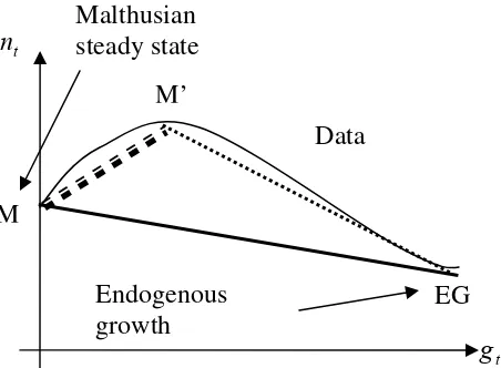
The empirical evidence and the predictions of the model regarding fertility and growth
are summarised in Figure 5. M andEG represent the steady-state Malthusian and
en-dogenous growth equilibria, respectively. The continuous hump-shaped line represents the
real-world evidence on the movement of fertility and growth in countries along the ”great
transition” (Galor, 2005). The dotted line (M ’ −EG) represents the negatively-sloped
saddle path (20); section (M −M ’) in Figure 6 (the broken line) is the instantaneous
jump at T.
To check that the model indeed fits the data, we have to ensure that fertility jumps temporarily (at the time of the shock) before settling on the lower endogenous growth
steady state level, n∗. From Figure 5, we have that the model produces such an inverted
U-shaped relation between fertility and growth if the absolute value of the slope of the
saddle arm (M ’ −EG) is higher than the slope of the locus (M −EG) represented by
the dotted line in the graph. Formally, we must have,
¯ ¯ ¯ ¯
nu−n∗
0−g∗
¯ ¯ ¯ ¯< ¯ ¯ ¯ ¯e nt e gt ¯ ¯ ¯ ¯= − N φ ,
where the first expression is the slope of (M −EG) and the last that of (M ’ −EG) in
Figure 5. Rearranging this expression, we can state that at the time of the shock, the
economy moves from the Malthusian equilibriumM onto the saddle path, (M ’−EG) if
nu < n∗+
(1−ε)e∗/(v+e∗)3+ [ε+ (1−ε)n∗e∗]/(v+e∗)2
1 +ε[1−n∗(v+e∗)]/[n∗(v+e∗)]
∙
g∗
φ
¸
. (21)
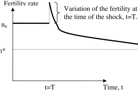
Under the assumption that (21) is satisfied, the dynamics of the fertility rate is represented in Figure 7.
Insert Figure 7
If (21) holds, (M−M ’) in Figure 6 is upward sloping, giving rise an upward jump of
fertility nt onto the stable arm; after that, nt will gradually decline towards its long-run
value in the endogenous growth regime, n∗. Thus, if this condition holds, a movement
can be predicted that can match the inverted U-shaped graph of fertility versus growth
found in the data. We assume that this condition holds without loss of generality, as we
have some degrees of freedom among the parameters. For example, from the results of
Proposition 1, we can see that the inverted relationship between fertility and income is
likely to happen if the innate level of skills of individuals, H0, and the cost in terms of
consumption good of raising children, f, are high. This is because higher values of these
parameters have a negative effect on the Malthusian steady-state number of children nu,
The reason why fertility can increase at the time of the shock is that an increase in the
level of human capital induces both an income and a substitution effect. While the income effect is positive because children are a normal good, the substitution effect is negative because the time allocated to bring up children can be used for the production of the
consumption good. When the level of human capital is low (as it is the case at the time
of the shock), the income effect dominates, leading individuals to bring up more children. However, as income (or human capital) rises, the costs of child quality increases as well.
For sufficiently high levels of human capital, the substitution effect will dominate leading the individuals to reduce the number of children they bring up. This is the standard
quality-quantity trade-offon children, represented by the move (M ’−EG) in Figure 6.
From the analysis above, we can note that the effects of status on the slope of the stable arm, (given by N/φ) is ambiguous. However, in the case where status makes the stable
arm steeper, the jump of fertility at T will be greater. Thus, the theoretical prediction
will be more pronounced, having the potential of matching the data more closely. In that
case, status can both decrease the basin of attraction around the Malthusian steady state
(see Sections 3.2.2-3.2.3), and change the dynamic path of the economy to match more
closely the facts about the “great transition”.
5
Conclusion
This paper has investigated the implication and importance of social aspirations for the
great transition in the BMT model. We have shown that social aspirations of people are a
possible factor that can contribute to a country’s switch to development. This is because
higher status motives increase the return to investment in children’s education relative
to the return to investment in the quantity of children. Moreover, we have argued that
there exist cases in which government authorities should postpone the introduction of
an economic policy, although such a policy aims to implement the social optimum. The
reason is that the policy could induce parents to substitute quantity for quality of children,
and thus it could break the process of economic development. Finally, the transitional
transition”.
Our framework can be extended in many ways. For instance, the analysis can be
extended to frameworks in which there is some social status accruing to children. On the
empirical side, an interesting issue would be to test our hypothesis regarding social status,
choice of fertility and education in order to measure its impact on economic growth.
6
Appendix
The Malthusian steady-state
As explained in the text, a Malthusian steady state is a corner solution. Adult
indi-viduals choose not to invest in education of their children. One has et= 0 in all periods
which implies that economic growth is zero: Ht+1 = Ht = H0 in all periods. Then, the
levels of consumption and utility of any individual are respectively given byct=ct+1 and
Vt =Vt+1 in all periods. Equation (10) follows directly from equation (8) wherect =ct+1.
This condition must hold with strict inequality because we have a corner solution. To
compute (9), we use (1), (5) and the fact that ct=ct+1 and Vt=Vt+1 in all periods.
The growing steady-state
When growth is strictly positive, the level of innate human capital of an individual,H0,
and thefixed cost of raising a child in terms of the consumption good,f, become negligible in the long-run (as ratios overHt). Thus, we can skip these variables in the computation
of the steady-state. From (3) and (2), one has 1 + g∗ = c
t+1/ct = Ht+1/Ht = φe∗
at the steady state. Using the fact that equation (6) reads with equality with strictly
positive investments in education and combining this equation with (5) one gets after
some manipulation
Ht+1
Ht
=φe∗ = φ(v+e
∗)
(1−ε)
dVt+1
dHt+1
Ht+1
Vt+1
. (22)
Since the growth rate of human capital and consumption are the same at steady-state,
one has
dVt+1
dHt+1
Ht+1
Vt+1
= dVt+1/Vt+1
dHt+1/Ht+1
= dVt+1/Vt+1
dct+1/ct+1
= dVt+1
dct+1
ct+1
Vt+1
Assuming that the economy has reached the steady-state, recursive substitution leads to
Vt+1 =
[(ct+1)Ψ(ct+1/ct+1)γ]1−σ
1−σ
P £
α(n∗)1−ε(1 +g∗)1−σ¤i. (24)
Thus, from the above equation we have that
dVt+1
dct+1
ct+1
Vt+1
= (1−σ)(1 +γ∆). (25)
Plugging the above result in (22), one gets e∗.Then, using (8) which holds with equality,
one deduces n∗.
The intermediate steady-state
Using (8) with the fact thatct+1 =ct in all periods, one gets (14). Using (5) with the
fact that growth is zero, one gets (15). Since the level of human capital is such that
Ht+1 =Ht =Hb in all periods, one gets (16) by using (2).
Optimal taxation
To compute the optimal tax, we first characterize the optimum. This is given by the individuals’s maximization problem stated in section 3.1 in which we setγ to zero. This is
because at optimum, the social planner takes into account that individuals are identical:
ct = ct. Her problem is to choose lt, et, nt, Ht+1 that maximize Vt = [(ct)Ψ(1)γ]1−σ/(1−
σ) +α(nt)1−εVt+1, subject to (2), (3), (4). This problem is equivalent to maximize (1)
with γ = 0, subject to the same constraints.
Second, to find the optimal tax rate, we must take into account that the resource constraint (3) becomesTt+lt(Ht+H0) = (1 +τt)ct+fnt.Following the same steps as in
Section 3.1 and comparing the set of first order conditions with the optimum conditions, one gets Proposition 2.
Transitional dynamics
Combining (5) and (6) (with equality in (6) as we are considering the endogenous
growth case of et >0), we get
(1−ε)Vt+1
[Ht(v+et) +f]φ
= dVt+1
dHt+1
which is a differential equation in Vt+1 anddVt+1/dHt+1. The solution is:
Vt+1 =Υtexp
∙
(1−ε)Ht+1/φ
Ht(v+et) +f
¸
,
where Υt is a variable independent of Ht+1 that must grow at the same rate as (ct)1−σ.
Indeed, plugging back the above equation in (5), we get
α(1−ε) (nt)−εΥtexp
∙
(1−ε)Ht+1/φ
Ht(v+et) +f
¸
= [Ht(v+et) +f] [1 +γ∆] (ct)−σ[Ψ(1)]γ(1−σ),
where Υt is a variable independent of Ht+1. For simplicity, we specify Υt = (ct)1−σ so
that both sides grow at the same rate. Taking a Taylor expansion of this equation and
dividing by the reference values (asymptotic steady-state of perpetual development), we
get
−εnet
n∗ +
(1−ε)v
(v+e∗)2eet=eht+ e
et
(v+e∗)2 −ect, (26)
whereect = (ct−c∗t)/ct∗ andent = (nt−n∗)/n∗.
Then, combining (3) and (4), and proceeding in the same way as before, we get
eht=ect+
(v+e∗)en
t+n∗eet
1−n∗(v+e∗) . (27)
Finally, linearisation of (2) yields
e
ht+1 =
φeet
1 +g∗ +eht, (28)
and linearisation of (8) yields
σ(ect+1−ect) =−
εent
n∗ −
v
1−vn∗net+1. (29)
Equations (26), (27), (28) and (29) is a 4×4 system in deviation from the reference
paths for fertility, time allocated to schooling, consumption and human capital. Now,
the strategy is to reduce this system to a 2×2 system in deviation from the reference
paths for time allocated to school and human capital. To do it, we use (26) and (27) to
eliminateectandent, and re-write the system in terms ofeht andeet.From (27), we can write
e
nt as a function of the other variables. Plugging the result in (26) yields the deviations
e
ct =eht+Meet, (30)
with
M ≡ (1−ε)e∗/(v+e∗)
2
1 +ε[1−n∗(v+e∗)]/[n∗(v+e∗)] >0.
Combining (30) with (27) yields (19) given in the text. Straightforward manipulations of
7
Reference
Abel, A.B., 1990. Asset prices under habit formation and catching up with the Joneses.
American Economic Review 80, 38-42.
Barro, R.J., 1991. Economic growth in a cross section of countries. Quarterly Journal
of Economics 106, 407—443.
Barro, R.J., G.S. Becker, 1988. A Reformulation of the Economic Theory of Fertility.
Quarterly Journal of Economics 108, 1-25.
Barro, R.J., G.S. Becker, 1989. Fertility Choice in a Model of Economic Growth.
Econometrica 57, 481-501.
Becker, G.S., 1991. A Treatise on the Family. Cambridge, MA: Harvard University
Press.
Becker, G.S., K.M. Murphy, R. Tamura, 1990. Human capital, fertility, and economic
growth. Journal of Political Economy 98, S12—S37.
Black, S.E., C. Juhn C., 2000. The Rise of Female Professionals: Are Women
Re-sponding to Skill Demand ? American Economic Review 90, 450-455.
Clark, A.E., A.J. Oswald, 1996. Satisfaction and comparison income. Journal of Public
Economics 61, 359-381.
Corneo, G., O. Jeanne O., 1997. On relative wealth effects and the optimality of growth. Economics letters 54, 87-92.
Crafts, N., T. Mills T., 2007. From Malthus to Solow: How Did the Mathusian
Economy Really Evolve? Working paper, University of Warwick.
Dixon, H.D., 2000. Keeping Up with the Joneses: Competition and the Evolution of
Collusion. Journal of Economic Behavior and Organization 43, 223-238.
Doepke, M., 2004. Accounting for Fertility Decline during the Transition to Growth.
Journal of Economic Growth 9, 347-383.
Dolado, J., F. Felgueroso, J.F. Jimeno, 2001. Female Employment and Occupational
Changes in the 1990s: How is the EU Performing Relative to the US? European Economic
Review 45, 875-879.
Literature from Malthus to Contemporary Models of Endogenous Population and
En-dogenous Growth. Journal of Economic Dynamics and Control 21, 205-242.
Fershtman, C., K.M. Murphy, Y. Weiss, 1996. Social Status, Education and Growth,
Journal of Political Economy 104, 108-132.
Fisher, W.H., F.X. Hof, 2000. Relative consumption, Economic Growth and Taxation.
Journal of Economics 73, 241-262.
Futagami, K., A. Shibata 1998. Keeping one step ahead of the Joneses: Status, the
dis-tribution of wealth, and long run growth. Journal of Economic Behavior & Organization
36, 109-126.
Galor, O., 2005. From Stagnation to Growth: Unified Growth Theory, Chapter 4 in Aghion, P. and Durlauf, S. (eds.), Handbook of Endogenous Growth.
Galor, O., D.N. Weil, 1999. From Malthusian Stagnation to Modern Growth.
Ameri-can Economic Review 89, 150-154.
Greenaway, D., Morgan, W., Wright, P., 2002. Trade liberalisation and growth in
developing countries. Journal of Development Economics 67, 229— 244.
Hopkins, E., T. Kornienko, 2004. Running to Keep in the Same Place: Consumer
Choice as a Game of Status. American Economic Review 94, 1085-1107.
Hall, R.E., 1988. Intertemporal Substitution in Consumption. Journal of Political
Economy 96, 330-57.
Kodde, D.A., J.M.M Ritzen, 1984. Integrating Consumption and Investment motives
in a Neoclassical Model of Demand for Education. Kyklos 37, 598-605.
Ljungqvist, L., H. Uhlig, 2000. Tax Policy and Aggregate Demand Management Under
Catching Up with the Joneses. American Economic Review 90, 356-66.
Long, N.V., K. Shimomura K., 2004. Relative Wealth, Status Seeking and
Catching-up. Journal of Economic Behavior & Organization 53, 529-542.
Lucas, R.E., 1988. On the Mechanics of Economic Development. Journal of Monetary
Economics 22, 3-42.
Mankiw, N.G., D. Romer, D.N. Weil, 1992. A contribution to the empirics of economic
growth. Quarterly Journal of Economics 107, 407—437.
Mokyr, J., 2000. Knowledge, Technology, and Economic Growth During the
Growth, The Hague, Kluwer; also available from the authors website, Northwestern
Uni-versity.
Oosterbeek, H., D. Webbink, 1995. Enrolment in higher Education in the Netherlands.
De Economist 143, 367-380.
Pham, T.K.C., 2005. Economic growth and Status-seeking through personal Wealth.
European Journal of Political Economy 21, 407-427.
Rauscher, M., 1997. Conspicuous consumption, Economic Growth and Taxation.
Journal of Economics 66, 35-42.
Sheran, M., 2007. The career and family choices of women: A dynamic analysis of
labor force participation, schooling, marriage, and fertility decisions. Review of Economic
Dynamics 10, pp. 367—399
Stiglitz, J., 1998. More Instruments and Broader Goals: Moving Toward the
Post-Washington Consensus. WIDER Annual Lecture, Helsinki, Finland, January 7.
Tournemaine, F., 2008. Social aspirations and choice of fertility: why can status
motive reduce per-capita growth? Journal of Population Economics 21, 49-66.
Tournemaine, F., C. Tsoukis, 2008. Relative Consumption, Relative Wealth and
Growth. Economics Letters, forthcoming.
Tsoukis, C., 2007. Keeping up with the Joneses, Growth, and Distribution. Scottish
Journal of Political Economy 54, 575-600.
Williamson, J., 2000. What Should the World Bank Think about the Washington
1 +
t
[image:27.595.99.389.84.340.2]H
Figure 1: Steady state equilibria 0
t
H
Hˆ
t
t H
H +1 =
State of perpetual development
Malthusian steady-state
1 +
t
[image:28.595.100.389.94.357.2]H
Figure 2: Effect of social aspirations on the steady state equilibria 0
t
H
( )
oHˆ
t
t H
H +1 =
0
>
,
1γ
C
1,
γ
>
0
C
0
=
,
2γ
C
0 0,01 0,02 0,03 0,04 0,05 0,06
1951 1954 19571960 1963 196 6
1969 1972 1975 197819811984 1987 1990 19931996 1999 200 2
2005
HK IN KO MA PHI SI
[image:29.595.91.506.69.286.2]THA
Figure 4: Phase diagram for the system (17) t
h~
Stable arm
Steady-states
t
e
~ (0,0)
Education
e*
Jump at the time of the shock t=T.
e=0
[image:31.595.103.369.87.250.2]t=T Time, t
Growth
Figure 5b: Dynamics of the growth rate
Time, t t=T+1
g*
g=0
Figure 6: Phase diagram for the fertility rate and income growth t
g
Malthusian steady state t
n
M
Data M’
Endogenous growth
Fertility rate
Variation of the fertility at the time of the shock, t=T. nu
n*
[image:34.595.113.351.113.273.2]t=T Time, t