Power aspects of analysis of variance in various models

Power aspects of analysis of variance in various models.

KANJI, G. K.

Available from Sheffield Hallam University Research Archive (SHURA) at:

http://shura.shu.ac.uk/19895/

This document is the author deposited version. You are advised to consult the

publisher's version if you wish to cite from it.

Published version

KANJI, G. K. (1978). Power aspects of analysis of variance in various models.

Doctoral, Sheffield Hallam University (United Kingdom)..

Copyright and re-use policy

See

http://shura.shu.ac.uk/information.html

Sheffield Hallam University Research Archive

Sheffield City Polytechnic Library

ProQuest Number: 10697201

All rights reserved

INFORMATION TO ALL USERS

The quality of this reproduction is dependent upon the quality of the copy submitted.

In the unlikely event that the author did not send a com plete manuscript and there are missing pages, these will be noted. Also, if material had to be removed,

a note will indicate the deletion.

uest

ProQuest 10697201

Published by ProQuest LLC(2017). Copyright of the Dissertation is held by the Author.

All rights reserved.

This work is protected against unauthorized copying under Title 17, United States C ode Microform Edition © ProQuest LLC.

ProQuest LLC.

789 East Eisenhower Parkway P.O. Box 1346

POWER ASPECTS OF ANALYSIS OF VARIANCE

IN VARIOUS MODELS

by

G. K. KANJI, MISc. F .I.S . F.S.S.

A thesis submitted to the Council fo r National

Academic Awards fo r the degree of Doctor of Philosophy

m b r a r v x^.

'«/ &

J'S- ?

m o

-A C K N 0 W L E D G E M E N T S

I wish to express my sincere appreciation''to ; .

POWER ASPECTS OF ANALYSIS OF VARIANCE IN VARIOUS MODELS

Summary

The object of the present work is to study the robust­ ness of the power in Analysis of Variance in relation to the departures from the in-built assumptions (i) equality of variance of the errors, (ii) statistical independence of the errors, and (iii) normality of the errors in fixed and random effects models. It is difficult if not impossible, to conduct an exhaustive study of the problem, because the above assump­ tions can be violated in many ways. However, a general model and some important particular models have been used to obtain fairly conclusive evidence regarding the robustness of the power in Analysis of Variance.

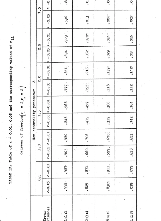
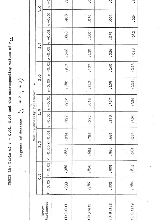
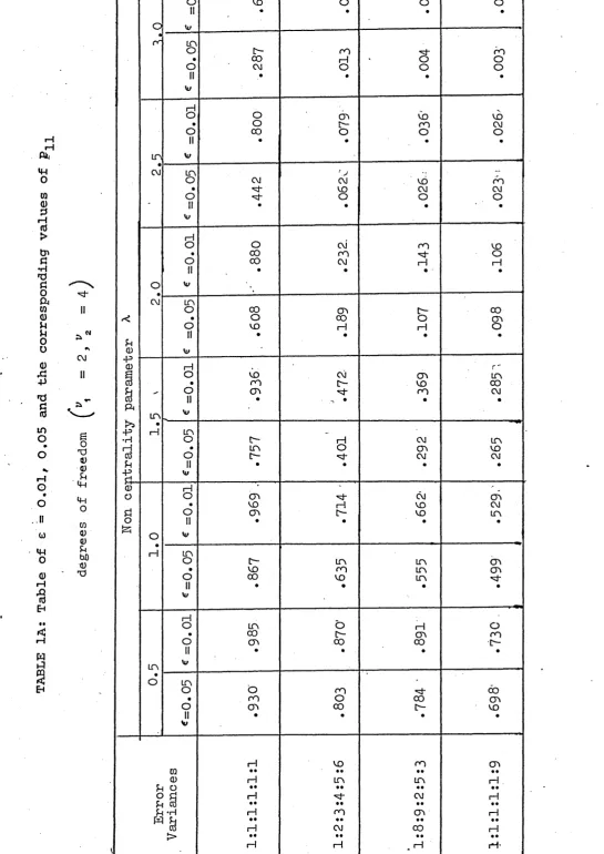
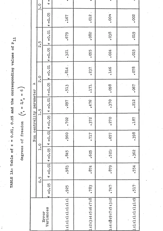
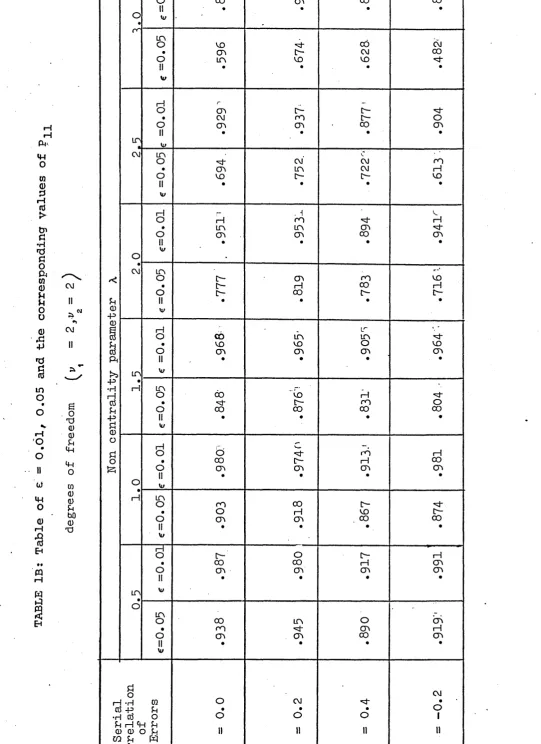
In order to obtain the power value in relation to the departure from the usual test assumptions, the general linear hypothesis model is considered. The power values when the assumptions of equality of variances and independence of errors are violated, are obtained and presented in Table IA and IB. The result suggests that in the above model, for tests regarding the inference about means, the power value is greatly affected by the inequality of error variances but only slightly affected by the serially correlated error variables. By using the permutation theory an approximate method is

Having studied the most general case in Analysis of Variance some particular models are discussed to investigate certain important aspects of the problem that are generated by these models.

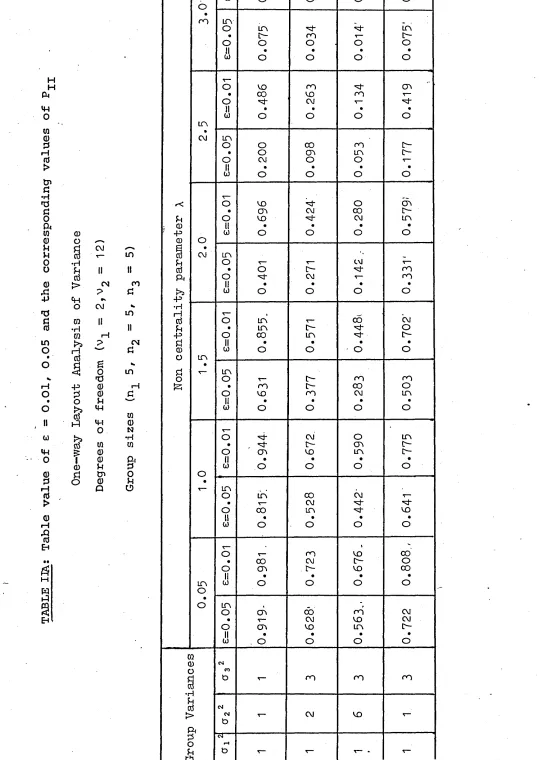
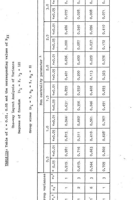
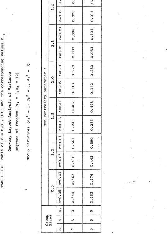
First of all fixed model one-way classification is con­

sidered to investigate whether it could show a different picture for unequal replication. The results so obtained are presented in Table IIA and IIB. They indicate that the power value is

greatly affected by the inequality of error variances and unequal group sizes. This procedure is easily modified to handle the random model.

Another particular case of the general linear model, that is fixed effect model two-way classification, is discussed.

The results so obtained are presented in Table IIIA and IIIB. They indicate that in two-way classification for the between Column

test, the power value is greatly affected by the inequality of column variances but only slightly affected by the serially correlated within rows error variables. Again this procedure is easily modified to handle the random model.

The use of simulation methods for calculating the power values in the case of non-normal errors is discussed. One and two-way classifications are considered for the fixed effect model. The Erlangian and contaminated normal distribution are taken as examples of a non-normal error distribution. The

results obtained by these methods are given in Table IVA and IVB which indicate that for the inference concerning means, the

power calculated under normal theory is only slightly affected by the non-normality of the errors.

Finally, the effect of non-normality on the power in analysis of variance for a random effect model is also discussed by a

simulation method. One and two-way classification are considered for this model and the Erlangian and contaminated normal

distributions are taken as examples of non-normality. The results obtained by these methods are given in Tables VA and VB which

indicate that non-normality has little effect on the power of the test.

G.K.K.

CONTENTS

Chapter 1.

(

1

.

1

)

(1.2)

(1.3) Chapter 2.

(

2

.

1

)

(

.

)

(2.3) (2.4) (2.5)

(

.

)

(3.1)

(3.2) (3.3) (3.4) Chapter 4.

(4.1) (4.2) (4.3) (4.4) Chapter 5.

(5.1)

(5.2) (5.3)

Page Introduction

Historical Background 1

Relationship of this thesis to earlier

work 4

Note 5

Power aspects in general linear model

Estimation of the Parameters 6

Test of Hypothesis 7

Distribution of the quadratic forms 9

Non-centrality parameter 11

Distribution of the ratio of quadratic

forms 11

Power of the test 12

Power aspects in general linear model1 by Pe rmu t a t ion The ory

Assumption and Test Criterion in general

linear model 14

Moments of the test criterion 15

Approximate distribution of test criterion 17

Power of the test 18

Power aspects in fixed and random effect models

Fixed model: one-way classification 20

Random model: one-way classification 23

Fixed model: two-way classification 26

Random model: two-way classification ... 31

Effect of Non-norma1i ty on the power: A simulation study

Simulation method and non-normal

distributions 34

Fixed model one-way classification 35

(5.4) Random model one-way classification 37

(5.5) Random model two-way classification . 39

Chapter 6. Discussion of the results and conclusions

(6.1) Power of the test in general linear model 41

(6.2) Power of the test in one-way classifi­

cation 44

(6.3) Power of the test in two-way classifi­

cation 44

(6.4) Power of the test by a simulation method

in a fixed model 47

(6.5) Power of the test by a simulation method

in random model 50

(6.6) Discussion of Results 50

(6.7) Areas for further research 51

References 52

Appendix A 56

Appendix B 58

Appendix C 60

Appendix D 63

Appendix E 66

Tables 68

1. INTRODUCTION

1.1 Historical Background

The assumptions usually associated with analysis of variance are that the errors in the measurements (i) have equal variances,

(ii) are statistically independent and (iii) are normally distributed.

Box (1953) introduced the term 'Robust* to denote a statis­

tical procedure which is insensitive to departures from assumptions underlying the model on which it is based. Such procedures are in common use, and several studies of robustness have been carried out in the field of 'Analysis of Variance'.

Numerous attempts have been made to study the effects of

departures from the usual test assumptions on Analysis of Variance techniques. For example, the effect of departure from normality in the distribution of the error term was studied for a one-way layout by Pearson (1931), Geary (1947) and Gayen (1950). David and Johnson (1951) considered the extent to which the non­

normality of the error distribution affects the F test. The test in general has been found very insensitive to non-normality of

errors. Welch (1938) studied the effect of unequal group variances on the 't' test. His results indicate that when the groups are of

equal size the effect is small, but this effect becomes larger when the groups are of unequal size. Hsu (1938(a)) also attempted to find the exact probability for this case. Gronow (1951) carried out the

special case of the one-way layout. The method used by David & Johnson is only approximate.

Box (1954(a), (b)) discussed the effect on tests of the null-hypothesis in Analysis of Variance of departures from the assump­ tions that errors (i) have equal variances and (ii) are statis­ tically independent. The result he obtained for the one-way layout shows that if the group variances are unequal, and group sizes are equal, then the test is not seriously affected. In the two-way layout, when the error variances are unequal from column to column, then there is an increased chance of exceeding the significance level for the test that column means are equal. For the corres­ ponding test on row means, the chance of exceeding the

significance level is decreased. For small differences in the variances neither effect is large. First order serial correlation within rows affects the between rows comparison more than the

between columns comparison.

Ito and Schull (1964) investigated the robustness of the o

Tq test in multivariate analysis of variance when variance and

co-variance matrices are not equal. They showed that, for large samples of equal size and moderate inequality of variance and co-variance matrices, the test is not seriously affected but that for unequal size the effects are quite large. Murphy (1967) used a simulation method for his study of the two sample test when the variances are unequal. His investigation indicates that the

permutation test and 't1 test are virtually identical in practice and are fairly robust to inequality of variances as long as sample sizes are equal.

homogeneous positive quadratic forms has been discussed in detail by Robbins (1940), Robbins and Pitman (1949) ,

and Hotelling (1948).

The more difficult distributions of non-homogeneous

quadratic forms have been investigated by Solomon (1961). Ruben (1962) has obtained a very general result, expressing the

distribution of both homogeneous and non-homogeneous quadratic

forms as an infinite linear combination of chi-square distributions with arbitrary scale parameters. He has also expressed the non-homogeneous quadratic form as an infinite linear combination of

non-central chi-square distributions with arbitrary scale parameters.

Box (1954) discussed the effect on tests of null-hypothesis in analysis of variance when the in-built assumptions other than the normality of errors are violated. He has ennunciated certain theorems concerning the distribution of relevant quadratic forms and applied his results to determine the effect of inequality of group variances in one way layout.

The permutation theory which provides a method for deriving robust criteria was first discussed by Box and Andersen (1955). When the errors are non-normal, Box and Watson (1962) developed an approximate method for studying the robustness of the

regression test in the null-hypothesis case. Through an

1.2 Relationship of this thesis to earlier work

In this thesis with the help of certain theorems due to Ruben (1962), a distribution of the ratio of two independent

quadratic forms is obtained and has been referred to as a general­ ised incomplete beta distribution. It is then applied to invest­ igate the effect of unequal error variances and serially correlated

errors on the power in the general linear model, in one-way and

two-way layout analysis of variance for fixed and random effect models.

This thesis differs from most other works in this field in that it is concerned with the direct approach and is more accurate than those of previous authors. In particular, it is shown that Tang's (1938) result for the power of the test can be easily obtained as a special case.

Using permutation theory and the generalised incomplete Beta distribution introduced earlier, a convenient method is devised to calculate the power values for the general linear

hypothesis model. Unlike others this method provides power values for a desired non-centrality parameter and degrees of freedom to study the robustness in analysis of variance. In particular it is shown that the Welch (1938 page 152) result for the variance of E^ for a limited population can be easily obtained as a special case.

In this thesis, unlike the previous authors (i.e. Geary,

Gayen, David and Johnson) a simulation method is used to investigate the sensitivity of the power of the test for the non-normality of the error distribution in one and two-way layout analysis of variance. Both fixed and random effect models are considered and the

non-normal distributions.

1.3 Note

POWER ASPECTS IN GENERAL' LINEAR MODEL

2•1 Estimation of the parameters

The general linear model of full rank can be written as

y = xB + e

(

2

.

1

.

1

)

where y is a (n x 1) vector of observations, x is a (n x p) matrix of known coefficients (p£n), 3 is a (p x 1) vector of parameters and e is a (n x 1) vector of 'error' random variables.

An assumption which is made on the e vector of random

variables is that e is distributed as N(o,cr2I) where I is a (n x n)

unit matrix and a 2 is unknown.

In order to investigate the effect of a departure from the usual test assumptions on the power in Analysis of Variance, we will consider the vector e such that e is distributed as N(0,cr26) where 6 is an (n x n) unknown positive definite symmetric matrix and a2 a scale factor. This will allow for both heteroskedasticity

(differing diagonal elements of 6) and interdependence (non zero off diagonal elements of 6) of the errors. Since the errors are normally distributed with expectation zero and variance covariance matrix of a26, the sum of squares that would appear in the exponent of the likelihood function is

This exponent will have to be minimized in order to maximize the' likelihood function.

The likelihood equation is given by

-~2- {(y-x3)* S”1 (y-x3)}

/ Q Arf A/

n 2

f(e,3 o 2 6) _n Exp " £xg) ' (ty - txg)_2a2

(

2

.

1

.

2

)

When 6 1 = t't, since any symmetric matrix can be split up into the product of triangular matrices, the maximum likelihood

estimates of 3 and a2 are

$ = (x’6-1x)-1x ,a"1y (2.1.3)

and

(ty-tx3)1(ty-tx3)

$2 = — — . — ... (2.1.4)

n

A

since E(3) = 3r then 3 is an unbiased estimate of 3. It can_{<w ^}

also be proved that E(a2) = ^I^a2 and therefore a2 is a biased_n

estimate of a2. But

(ty-tx3) '(ty-tx3)

2 n _ 2 Kin. 1 r \

a = a = --- _{n-p n-p} (2.1.5)

is an unbiased estimate of a2.

2.2 Test of Hypothesis

Testing the hypothesis 3 = 3* in the model (2.1.1) is equiv­ alent to testing simultaneously that each 3^ equals a given

constant 3|. In testing the hypothesis Hq : 3 = 3* it is

essential to devise a test function. For the evaluation of the power of the test, it is also necessary to know the distribution of the test function when the alternative hypothesis H-^: 3 ^ 3 * is true. Also we can test any sub-hypothesis y = y* where the elements of y constitute a subset of the parameters and those of the y* are given constant, (see, for example, Graybill (1961)p.l35) This can be seen in a following chapter which will examine one-way and two-way layouts.

L =

Vo + VE

(

.

.

)

where V = (ty_U -tx3)'(ty-tx3), V = (tx3-tx3*)1(tx3-tx3*)_{^ ^ A/ AS *V ^ AS As i l l ^ ^ «V «W«S,}

Let,

V.

T = E_V .(tx3-.txB*:) \(tx3.-tx3*)^ ^ ^ ^ AS As As AS AS AS

(ty-tx3)1(ty-tx3)

(

.

.

)

Since M-, = tx(x't'tx) ^ x't1 is an idempotent matrix._{JL I AS AS A/ AS AS AS AS As I}

We .therefore have

(ty-tx3*) 1 (ty-tx3*)

t = _{(ty-tx3*)'(I-M^)(ty-tx3*)} (2.2.3)

Let us denote the numerator and denominator of t as and q2

the two quadratic forms. In order to determine the rank of the

matrix which is also the rank of the quadratic form q^ we

proceed as follows

trace (M^) = tr. tx(x't'tx) -1 x't1 = p

Therefore the rank of is p and similarly the rank of (I-M^)

is n-p, and hence q^ and q2 are positive semidefinite quadratic

forms.

Since we are interested in knowing whether the two quadratic

forms q-^ and q2 are independent, we will express q-^ and q2 as

q, = (z - y) 'M, (z - y) and q = (z - y)'(I-M,)(z - y)_{J . AS AS J . fW AS AS AS AS AS AS AS1}

where z is an n-dimensional vector distributed as multivariate normal distribution with expectation zero and variance covariance matrix v and Mi is a positive semidefinite matrix, y being a given vector.

Now (z - y) 'I(z - y) = (z - y ) fM-,(z - y) + (z - y) ' (I - M-.) (z - y)

let H = £z, _{A/ «v«v} y = £n_{^ ^}

then (H - n) 1 (H - n) = (H - n) 1A (H - n) + (H - n) 1 (I - A) (H - n)

p n

= Z (H. - H.)2 + Z (H. - n.)2 (2.2.4)

i=l 1 1 i=p+l 1 1

so that the quadratic form (z - y)'M^(z - y) and (z - y) 1 (I - M^)(z-y)

are independent, i.e. the numerator q^ and denominator q2 of t are

mutually independent with rank p and (n - p) respectively.

2.3 Distribution of the quadratic forms

We now apply a theorem due to Ruben (1962) concerning the distribution of the quadratic form to find the distribution of q^ and q£. Now q^ can be expressed as

ql = fy ~ “ ^3*) (2.3.1)

where

M? = 6 ^x(x'6 ^x) ^x'6 ^

A/ X A/ ^

since the y's are distributed as N(xB/ V) we therefore have that.

¥**8 are distributed as N(0,V) where ¥* = y - xB. Hence substituting the value of y in (2.3.1) we have

q = (y*-y*) «M*(y*-y*) _{X »V ^ A/i.} (2.3.2)

where y* = (xB - xB*)

To achieve the required quadratic form for the application of Ruben (1962) theorem 1, we find that the linear transformation

changes the quadratic form to the canonical form given by

(x - b)'A(x - b) . Where x ’s are N(0,I) and N is the lower

-1 -1

triangular matrix defined by 6 = V = NN* and K is the

orthogonal matrix of the eigen vectors of N'M*N. The a^'s are the diagonal elements of the matrix A = K'N'M*NK and also the eigen values of N fM*N and b is a fixed n dimensional vector.

~ ~1~

Since q^ is a nonhomogenous quadratic form we can apply Ruben*s (1962) theorem 1 (Appendix A) and we see that

00

Hn',A,b,(a) = p Igl * “ 1 ^ CjXV+ajta/g)- (2.3.3)

where n 1 = p is the rank of matrix MJ, g is an arbitrary con­

stant and X2n+2 j is a chi-square distribution. Cj can be

calculated by the recursion relation given in the theorem. In equation

(2.3.3) the expression H ' _{n / A , d} is represented for b ^ 0 as a linear_^

combination of central x^^istribution function. The noncentrality

parameter (say X) which specifies the alternative hypothesis can be

obtained by using the vector b.

We now proceed to derive the distribution of the quadratic form q2? we have

q0 = (y - xB*)*M*(y - xB*) (2.3.4)

where

M* = S_1 - M*

Proceeding as for q^, we find that we can apply the Ruben (19 62) theorem 1 to find the distribution function of the quadratic

form q2 * But in this case the noncentrality parameter X is zero,

and we therefore have b = 0 and hence q2 is a homogeneous

-quadratic form. Applying theorem 2, we find that the distribu­

tion of q2 is

oo

Hn',A,0(a) = P[q2 * “] = j^odjx2n ,+2j(0l/g) (2.3.5)

2*4 Non c en trality1 Paramete r

It is always desirable to express the noncentrality parameter X in terms of y* and V. Therefore we proceed to relate the

b's in terms of y* and V where y**s and V's are as before.'

From the equations

¥* = NK'x y* = NKb

we have b = K ^ N ^ y * = .K,N"1y* (2.4.1)

where K is orthogonal matrix. Again we have

V"1 = N N 1 or N"1 = N'V_{A/ A/ A# A/ A» A^}

and hence

b = K ' N ^ y * = K ,N'V y* A/ A/ A# A/ a/ a/ a/ ’ A/

Now X2 = %(b'b) = %£bi2

b*b = y**V' NKK1N 1V y* = y**V' NN4 V y*

b 4b = y*1 V* y*

A# A/ A/ A/ A/

We' therefore obtain X2 = %bfb = %y*4V*y*_{A/ A# a/ a/}

2.5 Distribution of the ratio of quadratic forms

The distribution of q^ and q2 having been obtained in the

preceding section, we require the distribution of the ratio of

q ^ to q2 i.e. distribution of t . Since the g's in the equation

(2.3.3) and (2.3.5) are arbitrary scale parameters, we can take value of g equal to unity in all cases.

It can also be noted that q^ and q2 are independently

distributed as mixtures of central x2 's so that the ratio q ^ / q ^

Thus

00 oo

P(x = qi/q2 < a) = £ £ Cjd. Fp+2jjn_p+2i(^E|2ia) (2.5.1)

and Fv,t (.) is an F distribution.

2.6 Power of the test

As it is easier to compute the incomplete Beta function than the F distribution, we express the series in (2.5.1) in terms of incomplete Beta function with the help of the identity

Fm,n(x) = if5 h n )

where

I (.) is the incomplete Beta function._X

The series (2.5.1) then can be written as

p(x - q,/q2 < a) = E E C.d.I n~P+2i) (2.6.1)

j=o i=o ^

Where I (p/<2) is an incomplete Beta function.

Let G = l - L = — 1 T

1 + i _T 1 + T

then P(G s D) = P G ^ P £ D) = _{1 + T} P(t s y^-)_1-D

i.e.

P (G £ _{1 + a} ) = P(t £ a) if we put _{1 - D}D ■ = a

Hence,

00 00

= E E C.d.I a (£yi' SUStli) (2.6.2)

3=° 1=0 3

Let Pji be the type two error. Hence

P n = Z E CidiIu ^ 2 ' 2 } (2.6.3)

j=o i-o J o

1 + %

is a generalised incomplete beta distribution, where

u = _{o n-p e} F , and where e is the level of significance,₃

Therefore the power of the test is given by

00 00 .

e (A) = 1 -

Z I

j=° i=o J o

1+uo

POWER ASPECTS IN GENERAL LINEAR MODEL'BY PERMUTATION THEORY

3.1 Assumptions and Test Criterion

The general linear model of full rank can be written

Y = x3 + e (3.1.1)

where Y is a (nxl) vector of observation, x is a (nxp) matrix of

known coefficients (p £ n ) , 3 is a (pxl) vector of parameters and e is a (nxl) vector of error random variables.

An assumption which is made on the e vector of random

variables is that e is distributed as N(0,V) where V = a2I,_{<v fy •v}

I is a (nxn) unit matrix, and o 2 is unknown. The estimate 3 of 3

is then given by 3 = (x'x) x ’Y.

In testing the hypothesis 3 = 3* in the model (3.1.1) we shall use the likelihood ratio criterion

L =

VF

1 +

^

(3.1.2)

where Vn = (Y - xB) ' (Y - xB) , VF = (X B - xB*) ’ (x 8 " xB*) .

Let

VE

T = — =

V._o

(x3 - x3*) 1 (x.3 - x3*)

' (Y - x3) 1 (Y - x 3) (3.1.3)

which after simplification can be written as

(Y - x3*) *M(Y - xB*)

T = _{(Y - x.3*) ' (I~M) (Y - x 3*)} (3.1.4)

where M = x(x,x)’"1x , is a symmetric idempotent matrix.

that the D's are distributed as N(0,V) where D = Y - x$.

Substituting the value of Y in (3 .1 .4 ). we have

A/ *

V_ = (D - p*) 'M(D - p*)_Hi a# a* a> a» «v

where y* = x(3 -$*).

A*/ A/ #v

When the null-hypothesis is true the equation (3.1.4) is given by

D*M D

T D' (I-M)D (3.1.5)

Since the elements of D are the deviations from the mean we

therefore have D'l = 0, where 1 is the (nxl) vector, all of_{A/ A» A»}

whose elements are unity.

To study the shape of the distribution of the test criterion Z = 1 - L, and the power of the test when the errors are not

normally distributed we proceed as follows. We will assume like

Box and Watson (1962) that the vector e. in (3.1.1) are symmetrically_A/

distributed and hence the moments of the test criterion can be obtained using permutation theory. We will also assume that

x ^ = 1 for all the values of i.

3.2 Moments of the Test Criterion

Expressing the D's in terms of power sums

n r

i.e. Z D = V_{, u r}

u=l

VE

we have V, = 0 , V0 = D'D = + V_ and Z = — .

1 2 ~ ~ o E V2

To obtain the expectation of Z in the above situation we will first of all establish the required condition M 1 = 1, in the

Theorem

If X = (a|b) is a partitioned matrix where a is a (nxl) matrix,

b is a [nx(p-l)] matrix and M = X(X,X)"1X I is a symmetric

^ ^

idempotent matrix then the product Ma = a.

Proof

The Matrix M can be v/ritten as -l

M = (a |b) p-l (a|b) rcL_bT

M = (a|b) Ni a ' b'

- i

f * ^ _a1

b'a b'bJ |b'J Nj = constant= a

1

Since

Ma = (a b)

= (a|b)

N i a'b

b ’a b1 b

N i a'b

b1 a b'b

- 1

(a)

» 1 a'b

b'a b'b_{~ ~}

N b 1 a

- i

b1 a

Then

N b1 a

a'b b ' b

N (.b' a.)

when 0 is a null vector.

Therefore

'l Ma = (a | b) ^_{A/fV ^ A/ U ^} = a

therefore have a = 1 and hence M 1 = 1.

. Now using the relation M l = 1, we obtain (see Appendix C) the permutation mean as

e (z) = _(n- (3.2.1)

1 )

Also using David and Kendall's table (1949) and writing V2 and

in terms of Fisher K Statistics we obtain (see Appendix C) the permutation variance as

V (Z) = f (Ezf L|S=E 2. + t l / l L r fm - s L - 2 (p-1) (nrP_)l (3.2 .2)

(n-1 ) (n+1 ) (n-1 )^ _ n n(n+l) J

where m is the sum of squares of the diagonal elements of M. The result obtained in (3.2.2) has great similarity to the result given by Box and Watson (1962). Also with proper

grouping and substituting m = Z in (3.2.2) for one-way layout

analysis of variance we can easily obtain the value V(E2) by Welch (1938).

3.3 Approximate Distribution of Test Criterion

We know that when the elements of the error vector are normally distributed, the test criterion Z is distributed as a Beta distribution. We have assumed earlier that x ^ = 1 for all the values of i. Therefore the model (3.1.1) can be written as

Y = 1 Rx + X2 R2 + e (3.3.1)

given the following partition matrices,

and X = (1|X2) 52

Hence a test of the hypothesis R2 = R^ is required in the model

(3.-3.1)where R* is known. Following the method for the testing

buted and the null-hypothesis is true, the test criterion Z is distributed as a Beta distribution with (p-1) and (n-p) degrees of freedom, comparing the normal theory moments of Z with the permutation moments, we find that the mean is the same for both cases, whereas the variance differs. Pitman (1937) has shown that the third and fourth moments of the permutation distribution of Z agree closely with those of the Beta distribution. Hence the permutation distribution of Z could be approximated to a Beta distribution by adjusting the degrees of freedom. It could be readily shown that the approximating distribution has degrees of freedom d(p-l) and d(n-p) where

2 {n(n-1 ) . 2 - ( n - a h S ^ }

d =

(n-1 ){2 n (n-1 ) + (n-SJ S^S^}

K

si = K. 2 '

c = n(n-l) (n+1 )

2 (p-1) (n-p) (n-3) m - El _ n 2 (p-n(n+1 ) (n-p)1 )

Equivalently the permutation distribution of T could be approximated by an F distribution with degrees of freedom d(p-l) and d(n-p). The numerical value of d for a special case i.e. one-way layout Analysis of Variance could be easily obtained [see Johnson and Leone (1964)

p.2 1 ].

3.4 Power of the Test

Z = 1-L = —

i4 _T 1+T

and

or

P(Z < 0) = P T <

l+T =

P[T * iqr]

P(Z $ 7 3 — ) = P(T'$ a) if we put «r-~ = a

1 + a 1 - 0

When the errors are normally distributed then from the

equation (2.6.2) we have the test criterion Z as a Beta distribution with p-1 and N-p degrees of freedom. With the help of the theory developed in the preceding sections of this chapter we can now

approximate the distribution of Z (when the errors are not normally distributed) by Beta distribution, by adjusting the degrees of

freedom in the normal theory case.

Let P ^ ke the probability of type two errors. Hence

11

= V V c d JjL /d(P-l) + 2j d(n-p) + 2i. 4 1}

• ^ ■ n i 1 +a 2 ' 2 '

3=0 1=0

O* 1

where I (.) is an incomplete Beta distribution, a = —— F_{a n-p e}

and where e is the level of significance. Therefore the power of

the test is given by $(A) = 1 - P j . l m T^e non~centrality parameter

X and P^^ in (3.4.1) can be easily obtained by following previous chapter. We have thus found a practical method to study the effect of non-normality on the probability of type two errors in the

POWER ASPECTS IN FIXED AND RANDOM EFFECT MODELS 4.1 Fixed model; one-way classification

In certain circumstances, the group to group heterogeneity of variances may be obtained while testing the group to group

homogeneity of means in the one-way analysis of variance classification.

Suppose we have n^ observations in group i, i = l,2,...,k.

th — th

Denote by y . . the j observation in group i, by y. the i

group mean and y.. the grand mean. Suppose there are N observations allocated. Usually we assume,

Zn^y^ = 0 , and e^j are errors distributed normally and

independently about zero with the same variance a2. We retain the assumption of normality and independence but now assume variances

The sum of squares for the fixed effect model can be expressed

as Ch and Q2 where Ch is the within groups and Q2 the between groups

sum of squares.

We will first consider the distribution of Qi and 0 2. Here

Q2 is a quadratic form in yj. y 2. ... y^. and the matrix of the

quadratic form is

(4.1.1)

th

where £ + is the population mean from the i group,

O i 2 r O 2 2 , r f°r each group.

(4.1.2)

We may write the quadratic form Q2 = Y fB Y f where Y is the

A/ **

vector of normally distributed variables y.., with expectation

O 1 0 .- 2

£* and diagonal covariance matrix V = }

ni

Setting Z = Y -_^ a# ^

we may write this in the form Q2 = (Z + £*)*B(Z + £*) .

Since the elements of £* are deviations from the mean, the elements of Z are distributed with mean zero and variance V.

We shall transform the quadratic form to

Q 2 = (x-b)'A(x-b).

The transformation used is

Z = N K x C = “N K b (4.1.3)

and the elements of x are now normally distributed with zero

mean and unit variance. A is a diagonal matrix of the form

A = K'N'B N K, where K is the orthogonal matrix of eigenvectors of

N'B N and a.*s the diagonal elements of A are the eigen values of_{* * * * * * JL **}

N'B N. N is the lower triangular matrix V_{* * * * * * * * 0*} "” 1 = N N* . Thus the_{** **}

quadratic form Q2 or the between groups Sum of Squares can be

expressed as a non-homogeneous quadratic form. The distribution of

Q2 (see Section 2 .3 ) is given by

00

P(Q2 S a) = 5^ d jX2 p.+2j <f) (4.1.4)

where p* = k- 1 is the rank of the positive semidefinite quadratic

form B, g is an arbitrary constant and X2p»+2 j(*) a chi-square

P' P' J,

' 1 _ o . J . -s

0

d,. = e '2 E bj2 II (g/a±) 2

i=l i=l

where

P* P1 b. 2

hm = I (l-g/ai) ” 1 + mg I (-i ) (l-g/a. ) m - 1 m = 1 ,2 ,.

i=l i=l i

Similarly, Qi can be written as a quadratic form Z'D Z where Z is_{A/ A/ A/}

normally distributed with mean zero and variance V. By the transformation Z = N K Z the quadratic form Qi is reduced to X*A X where X's are normally distributed with zero mean and unit

variance and the a. 1 s are the latent roots of the matrix N fD N,

•L A/

where N and K are defined earlier and a. = cr2 . .

1 JL

The distribution of Ch is given by

P(Ql « a) = S CiX2N_k+2 i<f>' (4.1.5)

1 =U 3

where Ch can be obtained by the recursion relation given by i- 1

Ch = (2i) * " 1 E h. C i = 1,2,...

r=0 1“r r

C = n (g/a.)%

j=l 3

where h = Z (l-g/a.)n n = 1 ,2 ,...

j=l 3

The quadratic forms Qj and Q 2 are statistically independent, since

for each i, Y.. and_'

1

ni

Z (Y.. - Y..) are independently distributed.

j=l 3

The non-centrality parameter is given by

X = (%b’b)% = (%Eb.2)^ A/ 1 (4.1.6)

Proceeding as in Section 2.5 the distribution of the test criterion u is given by

Q2

P (u = — £ a) y 1

00 CO

where p* = k - 1, r' = N-k and F , ,(.) is the central F_{P fr}

distribution function, or

CO CO

P(u £ a) (4.1.8)

a generalised incomplete beta distribution, where

a = p ' / r ' F ^ , where e is the chosen level of significance.

Thus the probability of a type II error of magnitude p(u £ a / X ^ 0)

can be calculated from the equation (4.1.8) and given by

where the power of the test is B(X) = 1

-4.2 Random Model: One Way Classification

The situation may arise where a sample of K populations is drawn from a large set of populations. If we then consider that the K populations are randomly drawn from the large (possibly infinite) set of populations, then the model described by (4.1.1) changes to the Random effect model outlined below.

For example consider the determination of the effect of certain treatments on the nitrogen content of the tree leaves in an orchard. We select at random a group of trees, and then

choose a set of leaves at random from each selected tree. Let

y. . be the observed nitrogen content of the j* '*1 leaf from the i* ' * 1 tree

oo oo

j= 0 1 = 0 j i a 1 +g

then the structure of the model is given by

y . . = £ + y . + e . . _{^ lj} (4.2.1)_{v 7}

The general procedure for testing a hypothesis, and for

estimation with the random effects model is the same as with the fixed effect model. Scheff£ (1959) has discussed the power of the test when the error variances are equal and the lay out is

balanced. We will now discuss the power of the test in the

Random effects model when the error variances are unequal and the layout is not necessarily balanced.

In the model (4.2.1) we shall assume that y. and e . . are_{11 i j}

independent random variables, each with expectation zero and with

variances o ^ 2 and a^ 2 respectively. The a^ 2 (i = 1,2,...K) are

not necessarily equal. We shall also assume that the y^ and e^j are normally distributed.

Now the sums of squares that are involved are K n.

Ch =

z z

1

i=i j=i ^

and

K

Q i = £n.(y - y. . ) 2 (4.2.3)

i=l

Under the present model, the quadratic form

K n. K n.

Qi = I Z1 (y.. - y, ) 2 = Z Z1 (e.. - e. ) 2 (4.2.4)

i=l j=i i=l j=i 1

is the same as that for the fixed effect model, and thus the distri bution of Qi is also the same.

form in y lt y 2. ... y„. Namely Q2 = Y'B Y, where B is given in

X\ ^ ^

(4.1.2). Since the y.. are now distributed as N(£, o 2J + cr.2 I),

lj ~ y ~ 1 ~

we have that the y. are distributed as N(£, a 2J + d.2 /n.I).

1 ~ Y ~ l

The £'s are the same as in the fixed effect model, but the Y's

are now distributed as N(£, a 2J + a.2/n.I). When n^ = n, J is an

~ y ~ l l ~ j- ~

n x n matrix each element of which is equal to unity.

Setting Z = Y - £, we may express Q2 in the form

Q2 = (Z - £)'B(Z - £) where the Z's are distributed as N(0,V)

the variance-covariance matrix being V = (a 2J + a.2 /n.I).

We have seen in Section 4.1 that without loss of generality

the quadratic form Q2 can be reduced to the form Q2 where

Q2 = (x - b)'A(x - b) . The elements of x are standard normal

yariates. The distribution of Qj can then be obtained easily £nd is given by

0 0

P[Q5 S a] = S d. X 20 .+ 2 -i («/g) (4.2.5)

j=o 3 p

where p' is the rank of the positive semidefinite quadratic form B.

To test the hypothesis of equal treatment effects, we must Choose between the null and alternative hypothesis.

H0 ! “v2 = 0

Hj : c? Y 2 f 0 (4.2.6)

The power of the test for the situation (4.2.6) is then given

by 1 - where

PXI = PtQ.'2 /Q, .< «] = E E d( C.

1=0 1=0

where p* = K - 1, y1 = N K and a = £_{y ' e}7- F . e is the chosen level

of significance and d! ^ d^

4.3 Fixed Model - Two-way classification

Sometimes, when testing the k treatments in the n blocks in the two-way layout, circumstances arise where the variances of the k treatments differ from treatment to treatment. Similarly, when the experimental material is not homogeneous in mean from block to block, changes in variance may also occur from block to block.

The data given by Fisher (1958) on the frequency of rainfall at different hours in different months of the year, can be

classified as a two-way layout. Fisher has mentioned the strong serial correlation of the errors within months, since rainfall which continues for more than one hour is recorded in successive hours. The method of randomisation cannot be applied in this case.

Fisher has also remarked on the non-validity of the 1 between months*

comparison, due to the serial correlation between hours within months.

Let us consider a set of S values of the variate Y arranged in k columns and n rows where yti represents the value of the member belonging to the t ^ column and the i ^ row. We accept the usual assumptions that y ^ may be represented by a linear model

where EiJk = 0 , = 0 ? our assumptions concerning the e ^ will

be given later.

We shall represent the model in (2.1)' for all elements of th

the t column of the table (t = 1 ,2 ,...k) by

3ft. = 5in + $ + Ytin + St. (4.3.2)

where y. is the n x 1 vector, 1 is a n x 1 column vector all

♦v U • XI

of whose elements are unity, e, ' is the vector of errors and \Jj

is a n x 1 vector of row constants i, i}j2 , ... We shall

also use the notation _{~ i}y . . and e . . where y . . and e . . are_{~ l £ i ~ i}

th

respectively k x 1 vectors of observations and errors in the i

row of the table.

Instead of making the usual assumptions concerning the eti' name^y that they have the same variance and are

statistically independent, we shall also assume like Box (1954) that the e.^ are normally distributed with

E(eV.) _{~ i} = 0

E(e.. e.• .) = V_{~ ~ l}

The e.^ being mutually independent for i = l,2,...,n. Thus the

k variances and %k(k - 1 ) covariances are the same for every

row. This assumption permits us to study the effect of column to column inequality of variances and within row correlation of errors.

Box (1954) has shown with the help of the orthogonal transformation

H. . = Py. = £A + ¥ + Y4.A + E.

a, L • L « ** U •»<# ^ L •

(where P is the n x n orthogonal matrix, A = PI , ¥ = P$

the e . . and E . . are distributed in the same manner and E.. has_{ti ti ~ 1} the variance covariance matrix V. .

Now the sums of squares involved in the analysis of

variance two-way lay-out are

Q r = n Z (y. - y . .) 2

^ t=l

n

Q = k Z ( y ^ - y..) 2

i=l and

qe = * (yti ■ yt. - y - i + y - - ) 2

i=l t=l

where.Qcf and QE are the Between columns, Between rows and

Error sums of squares respectively.

l'-Using the transformation H. = n 2y . and H. = n2y.. the

tn u • n

sum of squares Q can be written as a quadratic form in H._{C ull •}

We can therefore express the quadratic form Q as H'C H where

1 i1 c ~ ~ ~

ft's are N(y, V) , C = (I, - and y = {£. - £}. Now setting

Y = H - y we will have that Qc = (Y + y)*C(Y + y) where the Y's

are N(0, V). The Qc can be then transformed to the form where

Qc = (x - b)'A(x - b) in which the x's are normally distributed with expectation zero and unit variance co-variance matrix. A is a diagonal matrix of the form A = K'M'CMK, where K is the orthogonal matrix of eigenvectors of M'CM and M is the lower triangular matrix

given by V” 1 = M M ' . The distribution of Q can then.be obtained

(see Section 2.3) and is given by

P (QC < o) = l a . x2p+2j (|) (4.3.3)

where p = k - 1 is the rank of the positive semi-definite

chi-square distribution. . dj can be calculated by the recursion relation given by

j-i

a.

z

a

j

J r=o J

P 0 P v

d = e 2 Z b*

n

° i=l 1 i=l 1

p m p b i

where h = Z (1 - g/a.)m + mg Z (-^) (1 - g/a. ) " 1" 1 m = 1,2,

i=l 1 i=l ai 1

and a. 1 s are the latent roots of the matrix M1 C M. The

non-centrality parameter X is equal to

X = (h b' _{~ -v} b)h = (h Z b?)% ■_JL

where b = K'M- 1 y.

We can write QE as the quadratic form in and in the

matrix notation express it as Z'C Z where C is the matrix given

1 l • ~ ~ ~

i i

by C = (1^, - ^— ). The E.^'s are distributed as N(0, V) and

Z's are similarly distributed with expectation zero and variance covariance matrix V.

In order to obtain the distribution of Z 1C Z we reduce this to the canonical form given by x'A x; the transformation used is Z = M K x, where the x's are normally distributed with zero mean and unit variance, and a^s are the latent roots of the matrix M' C M. (The matrix M and K were defined earlier.) The distribution of the homogeneous quadratic form Q _ .is then given by

p <QE < a) = J o ciXV a n n- i ^2 i (i } (4-3-4)

where C is a positive semi-definite matrix of rank k-1.

given by

i-1

C. = (2i)“1 I f. C i=l, 2,...

1 r= 0

Co = * (^/ a j ^

3=1

where f = Z (l“g/a-)m . 111=1 ,2 ,...

j=l

Box (1954) has proved that the quadratic form Q and Q_ are_{c E}

mutually independent whereas Qn and are not statistically

independent.

In order to find the distribution of the Between columns test criterion, we proceed as follows, Between column test

Q

criterion is given by u = — . Since the distributions of Q

UE c

and Qe are known, the distribution of u is found to be (see

section 2 .6 ).

P(u = ^ 2 * o) = s z d.C.I (n-1) ( k - D +2 1 )

QE j=0 i=0 3 1 T^- 2 z

1 +a

(4.3.5)

Thus the Type II error of magnitude P(u £ a/X ^ 0) can be calculated from the equation (4.3.5) and given by

Pjj = £ E (k-1+2j t (n-1 ) (k-l)+2 x) (4 .3 .6 )

i= 0 1 = 0 I S

where the power of the test is 3(X) = 1

-If we now consider the V matrix as diagonal, with unequal diagonal elements, then we have the case where variances change from column to column. The errors remain statistically independent,

Again, if the errors e 2± r ••• eki **-n ^ ie row are normally

distributed but not independently, then their variance covariance

matrix with unit diagonal elements and off-diagonal elements

is the coefficient of correlation between e, . and e .._{ti si}

We will consider the serial correlation which arises when the observations within columns or rows are made at equally

spaced intervals of time or space. \ .>.}/>:. t

4.4 Random Model; Two way classification

In the preceding section we have confined ourselves to the fixed effects model. We now consider a situation where the

treatments and Blocks are also random samples, from the population of treatments and Blocks respectively. This is the random effects model.

Consider the analysis of variance in the Two way layout of our Random effect model. The error variances may be unequal and errors are not necessarily uncorrelated. We will assume a model similar to that of the fixed effect case, namely

*ti = C + *i + Yt + eti (4.4.1)

But unlike for the fixed effect model we assume that iJk , y^, e ^

are three independent random variables. Further, and yt are

taken to be normally distributed with zero expectations and

variances o *I and a*I respectively.

Using the same notation in this model for all the elements

of the t ^ column of the table (t = l,2 ,...k) as for the fixed

Here the e.i are random normal variables with variance covariance

matrix E(e.. e..) = V. We also assume that the e . . (_~ j = 1,2,...n)

1 ~ 1 ~ ~ 3

follow the same distribution independently of the e... Let us_X

choose an n x n orthogonal matrix p, such that all the elements

-J-in the last row are n 2; transform-J-ing the Y. -J-into H • we f-J-ind that_{*** t . ~ t •}

H. = /n Y ._{~tn t}

Then

H. = p Y. = _{U **/ U •} + V + y.A + E. _{Li L •} (4.4.3)

where A , ¥ and E t are the same as in the fixed effect model.

We have seen in the earlier section that owing to the nature of the orthogonal matrix p, We can obtain the trans­ formed columns of the original two way table.

In the random effect model, unlike for the fixed effects model, y.does not vanish. The error sum of squares remains the same as in the fixed effect model case, i.e. the distribution of

Q„ in the Random effect model is the same as in the fixed effect_iii

model. The form of Qc is then given by K _

Q„ = n £ (y. - y. . ) 2

t=l

= _{, i tn} 2 (H.„ - -H. _n) 2

t=l

The sum of squares Qc can then be written in matrix notation as

a quadratic form in H _{~ m} The H's are distributed as N(y, V) where_{~ ~}

V = {a 2I + a2 6 }, and the 6 matrix in V is the positive definite

matrix which introduces the inequality of error variances and the correlation of errors.

Setting Y = H - y in the Quadratic form Q = H 1C H where_{-j. , ~ ~ C ~ ~}

C = (irr - y we have Q = (Y -t y)'C(Y + y) where the Y's

are distributed as N(0, _A/ V) . Again, with the help of an orthogonal

transformation, we can always transform the quadratic form Qc into the form (x - b)'A(x - b) where the x's are N(0, I). A is the diagonal matrix whose elements a^ are the latent roots of the

matrix N'c N, where V = N N'. The transformation _{^ A/ A# A/ A/ A#} used is

Y = N K x, _{A* A/ A» A/} y = N K b_{A/ A/ A,}

where K is the orthogonal matrix of the eigenvectors of N'C N. The distribution of the quadratic form Qc is then given by

oo

P[QC * a] = E dj X]^1+2j <“/g) (4 .4 .4 )

The d! s in (4.4.4) are not the same as those in (4.3.3) since

J

the V matrix has changed.

To test the hypothesis of equal treatment effects we choose between the null and alternative hypothesis.

H : a 2 = 0 (4.4.5)

o y

Hx: ay2 f 0

The power of the test for the situation (3.4.5) ’is then given

by 1 - Pjjf where

PII =

p [QC/QE

i

0

iio

3

1 +a

(4.4.6)

with p' = k- i, y» = (n-1 ) (k-1 ) , and a is the same as fixed

EFFECT OF NON-NORMALITY ON THE POWER: A SIMULATION STUDY

5.1 Simulation method and Non-normal Distributions

The effect of departure from normality in the distribution of the error term was studied for a one-way classification by Pearson

(1931) , Geary (1947) and Gayen (1950). David and Johnson (1951)_t

discussed the effects on the F-test as a result of the non-normality of the error distribution. The test in general was found to be

very insensitive to non-normality of errors.

In this chapter, unlike the previous authors, a simulation method is used to investigate the sensitivity of the power of

the test for the non-normality of the error distribution in one and two-way layout analysis of variance.

"Numerically, analysis of variance can be regarded as an algebraic decomposition of variation into different components. More specifically, it is concerned with observed data and the sum of squares of deviations of individual observations from their mean. The decomposition of this sum of squares takes account of various criteria of classification into which the data has been grouped.

The method of simulation does not give us the polished analytic results of mathematical theory but it helps us to duplicate the

observations resulting from a particular mathematical model, without first questioning the exact realism of the model used to fit data. Modern computing facilities have taken a leading role.in overcoming the tedious work involved in carrying out such simulation and it is justifiable to believe that concentrated research on simulation method will improve the reliability and usefulness of these

The calculation of power values in this thesis is carried out by the simulation method on an electronic computer by first

generating independent random variables uniformly distributed

on (0 ,1 ), and then allowing them to take the shape of the standard

normal, the Erlangian and the contaminated normal distribution.

The Erlangian random variable, X, which we shall consider here is defined as the sum of k independent negative exponential random variables each with parameter 0. Its distribution is of the form

k- 1

g(x)dX = e x ^ «' (k > 1, integer) (5.1.1)

k k

with the known mean and variance and ^ respectively.

The contaminated normal distribution which we shall consider is obtained as follows. Suppose we have two normal populations with the same mean, the first having h times the standard deviation of the second; if we mix populations by adding small amounts of the second to the first then we obtain a contaminated normal distribution. The probability density of such a distribution of contamination, c, and ratio of standard deviations, h, of the component normal distributions is given by

N h (z)dZ = (1-c) e_z /2dZ + c jjjL- e_z2/2h2dZ (5.1.2)

If c = 0, then (1) reduces to the standard normal distribution. The standard deviation of the distribution (1) is given by

/ch2-c+l.

5.2 Fixed Model: one-way Classification

th Let N observations be classified into s groups, the j

+* Vi

observation in the i group being y.jj. Instead of the usual_{-L J}

error follows (a) the Erlangian distribution, and (b) the

contaminated normal distribution. The sum of squares in the one-way

layout when the group sizes are equal (i.e. n) are given by

q = qi + q2 , where q is the total sum of squares, q2 the within sum

of squares and q2 the between sum of squares. The hypothesis and the

test criterion concerning the inference about the mean in the above situations are given by

Ho : Yi ~ °' Hi: Yi ^ 0 (i =

and

U “ q T T ^ i (5-2 -1}

When the are normally distributed and the null hypothesis

Hq is true, we have U distributed as a central F distribution with s-1 and N-s degrees of freedom. But when the alternative hypothesis

Hi is true then the power value 3 (1 ) is given by

B U ) = plu’ > fJ] (5.2.2)

where U* is a non-central F distribution, F is the value of F at_£

£ per cent level of significance, and X denotes the non-centrality

parameter.

The process of generating the random variables and finally the calculation of the ratio U* is repeated 2000 times. The power

value 3(X) is obtained by counting the number of times U1 is

s—i

greater than F£ and dividing the number by the total number of

repetitions. When the y^j follow the Erlangian distribution, or the

contaminated normal distribution, then the U1 will no longer be

distributed as a non-central F. The ratio U1 may, however, still