Munich Personal RePEc Archive
The Maastricht Criteria and Optimal
Monetary and Fiscal Policy Mix for the
EMU Accession Countries
Lipinska, Anna
Universitat Autònoma de Barcelona
June 2008
The Maastricht Criteria and Optimal Monetary and Fiscal Policy
Mix for the EMU Accession Countries
Anna Lipi´nska
yMay 2008
Abstract
The Maastricht convergence criteria set constraints on both monetary and …scal policies in the EMU Accession Countries. This paper uses a DSGE model of a two sector small open economy with distortionary taxes to address the following question: How do the Maastricht convergence criteria modify an optimal monetary and …scal policy mix in an economy facing domestic and external shocks?
We …nd that targets of the unconstrained optimal monetary and …scal policy are similar to those of the optimal monetary policy alone. The constrained policy is characterised by additional elements that penalize ‡uctuations of monetary and …scal variables around the new targets which are di¤erent from the steady state of the unconstrained optimal monetary policy.
Under the chosen parameterization (which aims to re‡ect the Czech Republic economy) the optimal monetary and …scal policy violates three Maastricht criteria: on the CPI in‡ation rate, the nominal interest rate and de…cit to GDP ratio. Both the stabilization component and deterministic component of the con-strained policy are di¤erent from the unconcon-strained optimal policy. Since monetary criteria play a dominant role in a¤ecting the stabilization process of the constrained policy, CPI in‡ation and the nominal interest are characterised by a smaller variability (than under the unconstrained policy) at the expense of a higher variability of de…cit to GDP ratio. The constrained policy is characterised by a de‡ationary bias which results in targeting the CPI in‡ation rate and the nominal interest rate that are lower by 1.3% (in annual terms) than the CPI in‡ation rate and the nominal interest rate in the countries taken as a reference. The constrained policy is also characterised by targeting surplus to GDP ratio at around 3.7%. As a result the policy constrained by the Maastricht convergence criteria induces additional welfare costs that amount to 60% of the initial deadweight loss associated with the optimal policy.
JEL Classi…cation: F41, E52, E58, E61.
Keywords: Optimal monetary and …scal policy, Maastricht convergence criteria, EMU accession countries
I would like to thank Kosuke Aoki for his excellent supervision and encouragement. I also thank Gianluca Benigno for helpful comments and suggestions. This work was undertaken as part of my International Doctorate in Economic Analysis, Universitat Autonoma de Barcelona, Spain, and was written during my stay at the Centre for Economic Performance, London School of Economics and Political Science, United Kingdom. It was not connected in any way to the Bank of England’s research program, and therefore does not necessarily re‡ect the views of that institution.
yBank of England, Monetary Analysis, International Economic Analysis Division, Threadneedle Street, London EC2R 8AH,
1
The introduction
Monetary policy has been used as the main stabilization tool in many countries. Interestingly, EMU accession countries, on their way to EMU, face the Maastricht criteria that put serious constraints on their monetary policies (as it was analyzed in Lipi´nska (2008)). Speci…cally, the countries should achieve a high and durable degree of price stability, which is, in quantitative terms, re‡ected in low in‡ation rates and low long term interest rates. Additionally, nominal exchange rates of the EMU accession countries versus the euro should stay within normal ‡uctuation margins. At the same time, …scal policy that could be seen as an additional stabilization tool is bound by the restrictions imposed in the Stability and Growth Pact. Accordingly, these countries should be characterized by a sustainable government …nancial position which is de…ned in terms of upper limits on de…cit to GDP ratio and debt to GDP ratio. At the moment many EMU accession countries do not satisfy some of the criteria.1
In this context a number of questions arise: Can …scal policy serve as an additional stabilization tool in the presence of restrictions set on monetary policy? How does this ability of …scal policy to mitigate business cycles change when faced with …scal constraints as well? In general, what should be the optimal monetary and …scal policy that satis…es all the Maastricht criteria? And …nally, which criteria: …scal or monetary ones put stronger constraints on stabilization macroeconomic policies?
To this purpose, we develop a DSGE model of a small open economy with nominal rigidities, distortionary taxation and government debt exposed to both domestic and external shocks. The model is an extension of the framework constructed by Lipi´nska (2008) where …scal policy does not issue any debt and taxes are assumed to be lump sum. Importantly, as in Lipi´nska (2008) the production structure is composed of two sectors: nontraded and home traded sector. In that way, we want to take into account recent empirical literature both on OECD and EMU Accession countries that highlights the role of sector speci…c shocks in explaining international business cycle ‡uctuations (see e.g. Canzoneri et al. (1999), Marimon and Zilibotti (1998), Mihaljek and Klau (2004)). Finally, following Benigno and Woodford (2003) and Benigno and De Paoli (2006) monetary and …scal policy is conducted in a fully coordinated way by a single policy maker.
In this framework we characterize the optimal monetary and …scal policy from a timeless perspective (Wood-ford (2003)). As in Lipi´nska (2008), we derive the micro founded loss function using the second order approx-imation methodology developed by Rotemberg and Woodford (1997) and Benigno and Woodford (2005). We …nd that the optimal monetary and …scal policy (unconstrained policy) should not only target in‡ation rates in the domestic sectors and aggregate output ‡uctuations but also domestic and international terms of trade. Subsequently, we present how the loss function changes when the monetary and …scal policy is constrained by the Maastricht convergence criteria. We derive the optimal monetary and …scal policy that satis…es all the Maastricht convergence criteria (constrained policy). Importantly, the Maastricht convergence criteria are not easily implementable in our model. Here we take an advantage of the methodology developed by Rotemberg and Woodford (1997, 1999) for the analysis of the zero bound problem and adapted by Lipi´nska (2008) for the analysis of the monetary criteria. This method enables us to verify whether a given criterion is satis…ed by only computing …rst and second moments of a variable for which the criterion is set.
1Lipi´nska (2008) reports that Bulgaria, Estonia, Hungary, Latvia, Lithuania, Romania and Slovakia fail to ful…ll the CPI in‡ation
Under the chosen parameterization (which aims to re‡ect the Czech Republic economy) the optimal monetary and …scal policy violates three Maastricht convergence criteria: on the CPI in‡ation rate, the nominal interest rate and de…cit to GDP ratio. Both the stabilization component and deterministic component of the constrained policy are di¤erent from the unconstrained optimal policy. The constrained policy leads to a smaller variability of the CPI in‡ation and the nominal interest rate and at the same time higher variability of de…cit to GDP ratio. This re‡ects an active stabilization role of …scal policy in the presence of direct constraints on monetary instrument. Moreover, as in Lipi´nska (2008) the constrained policy is characterized by a de‡ationary bias which results in targeting the CPI in‡ation rate and the nominal interest rate that are lower by 1.3% (in annual terms) than the CPI in‡ation rate and the nominal interest rate in the countries taken as a reference. Importantly, the constrained policy is also characterized by targeting surplus to GDP ratio at around 3.7%. This result is determined by a relative dominance of the monetary criteria over the …scal ones in a¤ecting the stabilization process. Accordingly the constrained policymaker uses actively …scal instruments and in order to comply with all the criteria has to assign a relatively high surplus to GDP ratio target. As a result, the policy constrained by the Maastricht convergence criteria induces additional welfare costs that amount to 60% of the initial deadweight loss associated with the optimal unconstrained policy. These welfare costs have their origin in con‡icting interest of monetary and …scal criteria and also relatively poor performance of …scal policy as an additional stabilization tool.
The literature on the macroeconomic policies in the EMU Accession countries concentrated so far on the analysis of the monetary criteria and their impact on the appropriate choice of the monetary regime. In particular, Devereux and Lane (2003), Ferreira (2006), Laxton and Pesenti (2003) and Natalucci and Ravenna (2007) study this issue in a framework of open economy DSGE models.2
The issue of a proper design of …scal policy in the EMU Accession countries has not been studied up till now. However, theoretical literature addressed already the problem of a joint optimal monetary and …scal policy both in the closed, open economy and monetary union environment. Schmitt-Grohe and Uribe (2004) and Benigno and Woodford (2003) study the design of optimal monetary and …scal policy in the closed economy environment, while Benigno and De Paoli (2006) derive the optimal monetary and …scal policy for a small open economy. These papers …nd that variations in …scal instruments should serve the same objectives as those in the optimal monetary policy design, i.e. stabilization of in‡ation and the output gap that measures total distortion of the level of economic activity. Ferrero (2005), Gali and Monacelli (2008) and Pappa and Vassilatos (2005) are examples of papers that study optimal monetary and …scal policy in a monetary union. In particular, Ferrero (2005) shows that regional …scal policies that respond to a measure of real activity perform better in terms of welfare than balanced budget rules. Gali and Monacelli (2005) …nd that the lack of regional monetary instrument generates a stabilization role for regional …scal policies. Interestingly, Pappa and Vassilatos (2006) examine how general …scal rules that are designed to satisfy …scal criteria a¤ect macroeconomic stability and welfare in a two-region monetary union. They …nd that some ‡exibility in compliance with …scal criteria can be welfare improving.
We take advantage of these theoretical studies and characterize an optimal monetary and …scal policy mix in a model which tries to re‡ect some of the characteristics of the EMU Accession countries. Then we analyze the e¤ects of the Maastricht criteria on the optimal policies. In that way we can set guidelines on the way monetary and …scal policy should be conducted in the EMU Accession countries.
The rest of the paper is organized as follows: the next section describes the model. Section 3 explains
2Lipi´nska (2008) provides a detailed discussion of both empirical and theoretical papers on the monetary policy in the EMU
derivation of the optimal monetary and …scal policy. Section 4 presents the way we reformulate the Maastricht convergence criteria in order to implement them into our framework. Section 5 is dedicated to derivation of the optimal policy constrained by the Maastricht convergence criteria. Section 6 compares the unconstrained optimal monetary and …scal policy with the optimal monetary and …scal policy constrained by the Maastricht convergence criteria under the chosen parameterization of the model. Section 7 concludes.
2
The model
Our modelling framework is based on a two-sector SOE model of Lipi´nska (2008) and one-sector SOE models of De Paoli (2004) and Benigno and De Paoli (2006). Following De Paoli (2004), we model a small open economy as the limiting case of a two-country problem, i.e. where the size of the small open economy is set to zero. We consider two highly integrated economies where asset markets are complete. In each of the economies, there are two goods sectors: nontraded goods and traded goods. Each of the sectors (domestic and foreign) features heterogeneity of goods and monopolistic competition. Labour is the only factor of production and is mobile between sectors in each country and immobile between countries. We assume the existence of home bias in consumption which, in turn, depends on the relative size of the economy and its degree of openness. Although the law of one price holds, existence of home bias leads to deviations from the purchasing power parity.
As far as the monetary and …scal policy is concerned we follow Benigno and Woodford (2003) and Benigno and De Paoli (2006) and assume that the policies are conducted in a fully coordinated way by a single policymaker. The role for monetary policy arises through the introduction of monopolistic competition and price rigidities with staggered Calvo contracts in all goods sectors. The model features complete pass-through as prices are set in the producer’s currency. We abstract from any monetary frictions by assuming cashless limiting economies.3
The …scal policy issues a one period nominal non-state contingent debt which is …nanced only through the distortionary revenue taxes collected in both domestic sectors. On the contrary to Lipi´nska (2008) the lump sum taxes are not available.
Finally, the stochastic environment of the small open economy is characterized by asymmetric productivity shocks originating in both domestic sectors, preference shocks, foreign consumption shocks and government expenditure shocks.
2.1
Households
The world economy consists of a continuum of agents of unit mass: [0; n)belonging to a small country (home) and[n;1]belonging to the rest of the world, i.e. the euro area (foreign). There are two types of di¤erentiated goods produced in each country: traded and nontraded goods. Home traded goods are indexed on the interval
[0; n) and foreign traded goods on the interval[n;1], respectively. The same applies to nontraded goods. In order to simplify the exposition of the model, we explain in detail only the structure and dynamics of the domestic economy. Thus, from now on, we assume the size of the domestic economy to be zero, i.e. n!0.
Households are assumed to live in…nitely and behave according to the permanent income hypothesis. They can choose between three types of goods: nontraded, domestic traded and foreign traded goods. Ci
t represents
consumption at period t of a consumer i and Li
t constitutes his labour supply. Each agent i maximizes the
following utility function:4
3See Woodford (2003).
4In general, we assumeU to be twice di¤erentiable, increasing and concave in C
tand V to be twice di¤erentiable, increasing
maxEt0
( 1
X
t=t0
t t0 U Ci
t; Bt V Lit
)
; (1)
whereEt0 denotes the expectation conditional on the information set at datet0, is the intertemporal discount
factor and0< <1; U( )stands for ‡ows of utility from consumption andV( )represents ‡ows of disutility from supplying labour.5 C is a composite consumption index. We de…ne consumers’ preferences over the composite
consumption indexCt of traded goods (CT;t) (domestically produced and foreign ones) and nontraded goods
(CN;t):
Ct
1 C
1
N;t + (1 )
1 C 1 T;t 1 ; (2)
where > 0 is the elasticity of substitution between traded and nontraded goods and 2 [0;1] is the share of the nontraded goods in overall consumption. Traded good consumption is a composite of the domestically produced traded goods (CH) and foreign produced traded goods (CF):
CT;t
h
(1 )1C
1 H;t + 1 C 1 F;t i 1 ; (3)
where >0is the elasticity of substitution between home traded and foreign traded goods, and is the degree of openness of the small open economy ( 2[0;1]).6 Finally,C
j (wherej =N; H; F) are consumption sub-indices
of the continuum of di¤erentiated goods:
Cj;t
2 4 1
n 1 Zn
0
ct(j)
1 dj 3 5 1 ; (4)
where >1represents elasticity of substitution between di¤erentiated goods in each of the sectors. Based on the above presented preferences, we derive consumption-based price indices expressed in the units of currency of the domestic country:
Pt
h
PN;t1 + (1 )PT;t1 i
1 1
; (5)
PT;t
h
PH;t1 + (1 )PF;t1 i
1 1 (6) with Pj;t 2 4 1 n n Z 0
pt(j)1 dj
3 5
1 1
: (7)
5We assume speci…c functional forms of consumption utility U Ci
t , and disutility from labourV Lit : U Cti
(Cit)1 Bt
1 ;
V Li
t 'l( Li
t) 1+
1+ with ( >0), the inverse of the intertemporal elasticity of substitution in consumption and ( 0), the
inverse of labour supply elasticity andBt;preference shock.
6Following de Paoli (2004) and Sutherland (2002), we assume home bias ( ) of the domestic households to be a function of the
relative size of the home economy with respect to the foreign one (n) and its degree of openness ( ) such that(1 ) = (1 n)
Although we assume the law of one price in the traded sector (i.e. p(h) =Sp (h)andp(f) =Sp (f)where
S is the nominal exchange rate), both the existence of the nontraded goods and the assumed home bias cause deviations from purchasing power parity, i.e. P 6=SP . The real exchange rate can be de…ned in the following manner: RS SP
P :Moreover, we de…ne the international terms of trade asT PF
PH and the ratio of nontraded
to traded goods’ prices (domestic terms of trade) asTd PN
PT:
From consumer preferences, we can derive total demand for the generic goods – n(home nontraded ones),
h(home traded ones),f (foreign traded ones):
yd(n) = p(n)
PN
PN
P (C+G); (8)
yd(h) = p(h)
PH
PH
PT
(1 )(CT+GT) +
p (h)
PH
PH
PT (CT +GT); (9)
yd(f) = p (f)
PF
PF
PT (CT +GT) (10)
where variables with an asterisk represent the foreign equivalents of the domestic variables. Moreover, G
andG denote exogenous aggregate government expenditures which have the same composition as the private consumption. Accordingly, GT and GT denote government expenditure in the tradable sector. Importantly,
since the domestic economy is a small open economy, demand for foreign traded goods does not depend on domestic demand. However, at the same time, demand for domestic traded goods depends on foreign demand. Households get disutility from supplying labour to all …rms present in each country. Each individual supplies labour to both sectors, i.e. the traded and the nontraded sector:
Li
t=L i;H t +L
i;N
t : (11)
We assume that consumers have access to a complete set of securities-contingent claims traded internation-ally. Each household faces the following budget constraint:
PtCti+EtfQt;t+1Dt+1g Dt+WH;ti LiH;t+WN;ti LiN;t+
n
R
0
i N;tdi
n +
n
R
0
i H;tdi
n ; (12)
where at datet, Dt+1 is nominal payo¤ of the portfolio held at the end of period (t), Qt;t+1 is the stochastic
discount factor for one-period ahead nominal payo¤s relevant to the domestic household, H;t and N;t are
nominal pro…ts from the domestic …rms. Moreover, consumers face no Ponzi game restriction.
The short-term interest rate(Rt)is de…ned as the price of the portfolio which delivers one unit of currency
in each contingency that occurs in the next period:7
Rt1=EtfQt;t+1g: (13)
The maximization problem of any household consists of maximizing the discounted stream of utility (1) subject to the budget constraint (12) in order to determine the optimal path of the consumption index, the labour index and contingent claims at all times. The solution to the household decision problem gives a set
of …rst-order conditions.8 Optimization of the portfolio holdings leads to the following Euler equations for the
domestic economy:
UC(Ct; Bt) = Et UC(Ct+1; Bt+1)Qt;t1+1
Pt
Pt+1
: (14)
There is a perfect sharing in this setting, meaning that marginal rates of consumption in nominal terms are equalized between countries in all states and at all times.9 Subsequently, appropriately choosing the distribution
of initial wealth, we obtain the risk sharing condition:
UC(Ct; Bt)
UC(Ct; Bt)
= Pt
StPt
= RSt 1; (15)
where >0 and depends on the initial wealth distribution. The risk sharing condition implies that the real exchange rate is equal to the marginal rate of substitution between domestic and foreign consumption.
The optimality condition for labour supply in the domestic economy is the following:
Wk
t
Pt
= VL(Lt)
UC(Ct; Bt)
; (16)
where Wk is the nominal wage of the representative consumer in sector k (k = H; N):10 So the real wage is
equal to the marginal rate of substitution between labour and consumption.
2.2
Firms
All …rms are owned by consumers. Both traded and nontraded sectors are monopolistically competitive. The production function is linear in labour which is the only input. Consequently, its functional form for …rmiin sectork(k=N; H) is the following:
Yk;t(i) =AktLkt(i): (17)
Price is set according to the Calvo (1983) pricing scheme. In each period, a fraction of …rms(1 k)decides
its price, thus maximizing the future expected pro…ts. The maximization problem of any …rm in sectork at timet0 is given by:
max
Pk;t0(i)
Et0
1
X
t=to
( k)sQt0;t (1
k
R;t)Pk;t0(i) M C
k
t(i) Yk;td 0:t(i)
subject to Yd
k;t0:t(i) =
Pk;t0(i)
Pk;t
Yk;t; (18)
whereYd
k;t0:t(i)is demand for the individual good in sectork produced by produceri at timetconditional on
keeping the pricePk;t0(i) …xed at the level chosen at time t0; M C
k t =
Wtk(i)
Ak
t is the nominal marginal cost in
sectorkat timet, and k;t are revenue taxes in sectork.
8We here suppress subscript i as we assume that in equilibrium, all agents are identical. Therefore, we represent optimality
conditions for a representative agent.
9We have to point out here that although the assumption of complete markets conveniently simpli…es the model, it neglects a
possibility of wealth e¤ects in response to di¤erent shocks (Benigno (2001)).
1 0Notice that wages are equalized between sectors inside each of the economies, due to perfect labour mobility and perfect
Given this setup, the price index in sectorkevolves according to the following law of motion:
(Pk;t)1 = k(Pk;t 1)1 + (1 k)(Pk;t0(i))
1 : (19)
2.3
Government budget constraint
The government issues a nominal, non-state contingent debt denominated in domestic currency and taxes the revenue income of …rms in the nontraded sector at rate N;t and also in the home traded sector at rate H;t:
The revenues are spent on government expenditures (Gt) and interest payments on outstanding nominal debt.
We assume that there are no seigniorage revenues.
Government debt,Dt, expressed in nominal terms, follows the law of motion:
Dt=Rt 1Dt 1 Ptsrt (20)
wheresrtis the real primary budget surplus:
srt= N;tpN;tYN;t+ H;tpH;tYH;t Gt (21)
andpN;t PPN;tt andpH;t
PH;t
Pt denote relative prices. We de…ne:
dt
DtRt
Pt
(22)
in order to rewrite the government budget constraint as:
dt=dt 1
Rt
t
Rtsrt: (23)
The rational-expectations equilibrium requires that the expected path of government surpluses must satisfy an intertemporal solvency condition :
dt0 1
t0
UC(Ct0; Bt0) =Et0
1
X
t=t0
t t0U
C(Ct; Bt)srt: (24)
in each state of the world that may be realized at date t0:This condition restricts the possible paths that
may be chosen for the tax ratesf N;t; H;tg:Moreover, monetary policy can a¤ect this condition by in‡uencing
in‡ation in periodt0 and also a¤ecting the discount factors in subsequent periods. This condition is derived
from the household optimization condition (14) and law of motion of debt (23). As discussed in Woodford (2001) this condition serves as one of the constraints in choosing an optimal plan among possible rational-expectations equilibria.
2.4
Monetary and …scal policy
We approximate the model around a steady state in which exogenous shocks take constant values. Moreover steady state in‡ation is zero and tax rates are chosen in such a way in order to maximize welfare of the agents. The loglinearized version of the model is available in the Appendix.
3
The optimal …scal and monetary policy
Since our model is microfounded the optimal policy is de…ned as the policy that maximizes welfare of society subject to the structural equations of an economy.
We use a linear quadratic approach (Rotemberg and Woodford (1997, 1999)) and de…ne the optimal monetary policy problem as a minimization problem of the quadratic loss function subject to the loglinearized structural equations (presented in the Appendix). First, we present the welfare measure derived through a second-order Taylor approximation of equation (1):
Wt0 =UCCEt0
1
X
t=t0
t t0[z0
vvbt
1 2bv
0
tZvbvt bv
0
tZ bt] +tip+O(3); (25)
wherebv0
t=
h b
Ct YbN;t YbH;t bN;t bH;t
i
;b0t=h AbN;t AbH;t Bbt Cbt Gbt
i
;
z0
v=
h
1 sCYN sCYH 0 0
i
withsCYN
!YN
C - steady state share of nontraded labour income in
domestic consumption,sCYH
wYH
C - steady state share of home traded labour income in domestic consumption,
and matricesZv; Z are de…ned in Appendix B;tipstands forterms independent of policyandO(3)includes
terms that are of a higher order than the second in the deviations of variables from their steady state values. Notice that the welfare measure (25) contains the linear terms in aggregate consumption and sector outputs. These linear terms originate from di¤erent distortions in the economy. First, monopolistic competition together with distortionary revenue taxes in both domestic sectors lead to ine¢cient levels of sector outputs and also an ine¢cient level of aggregate output. Second, since government spends its revenues on government expenditures domestic consumption and aggregate output are not equalized. Third, openness of the economy can also result in trade imbalances, i.e. domestic consumption can be di¤erent from the aggregate output. Importantly, their composition depends on the domestic and international terms of trade. Finally, similarly to De Paoli (2007) and Lipinska (2008) there exists an international terms of trade externality that creates an incentive for policy to generate a welfare improving real exchange rate appreciation, i.e. disutility from labour decreases without an accompanying decrease in the utility of consumption.
The presence of linear terms in the welfare measure (25) means that we cannot determine the optimal policy, up to …rst order, using the welfare measure subject to the structural equations (presented in the Appendix) that are only accurate to …rst order. Following the method proposed by Benigno and Woodford (2005) and Benigno and Benigno (2005), we substitute the linear terms in the approximated welfare function (25) by using a second order approximation to some of the structural conditions.11 As a result, we obtain the fully quadratic
loss function which can be represented as a function of aggregate output (Ybt), domestic and international terms
of trade (Tbd
t;Tbt), domestic sector in‡ation rates (bH;t; bN;t) and revenue tax rates in the nontraded and home
traded sector (bN;t;bH;t). Its general expression is given below:
minLt0 = UCC 1
X
t=t0
t t0[1
2 y(Ybt Yb
T t )
2+1
2 Td(Tb
d
t TbtdT)
2+1
2 T(Tbt Tb
T t )
2+ (26)
1
2 N(bN;t b
T N;t)
2+1
2 H(bH;t b
T H;t)
2+
Y TdYbtTbtd+ Y TYbtTbt+ TdTTbtdTbt+ (27)
+bN;t( Y NYbt+ T NTbt+ Td NTb
d
t) +bH;t( Y HYbt+ T HTbt+ Td HTb
d
t) + (28)
+1
2 Nb
2
N;t+
1
2 Hb
2
H;t] +tip+O(3) (29)
whereYbT t ;Tbd
T
t ;TbtT;bTN;t;bTH;t are target variables which are functions of the stochastic shocks and, in general,
are di¤erent from the ‡exible price equilibrium processes of aggregate output, domestic terms of trade and international terms of trade.12 The termtipstands forterms independent of policy. The coe¢cients
Y; Td;
T; N; H; T Td; Y Td; Y T; H; N; Y N; T N; Td N; Y H; T H; Td H;are functions of the
structural parameters of the model.
Similarly to Lipi´nska (2008) our loss function generalizes previous studies regarding optimal monetary policy characterization in both closed economy environments (Aoki (2001), Benigno (2004), Rotemberg and Wood-ford(1997)) and open economy environments (Gali and Monacelli (2005), De Paoli (2007)). Moreover this loss function is also related to the literature on optimal monetary and …scal policy in the sticky price environment (Benigno and Woodford (2003), Benigno and De Paoli (2007), Schmitt - Grohe and Uribe (2003)). As in Be-nigno and Woodford (2003) and BeBe-nigno and De Paoli (2007) we obtain that variations in distortionary taxation should be chosen to serve the same objectives as those emphasized in the literature on monetary stabilization policy. Interestingly, our loss function also involves some stabilization of taxes.13
To simplify the exposition of the optimal plan we reduce number of variables to a set of eight domestic variables which determine the loss function (26), i.e. Ybt; Tbtd; Tbt; bH;t; bN;t; bN;t; bH;t; dbt: In Appendix we
present the structural equations of the two-sector small open closed economy in terms of these variables. Finally, the policy maker following the optimal plan under commitment choosesfYbt;Tbtd;Tbt;bH;t;bN;t;bN;t;bH;t;dbtg1t=t0
in order to minimize the loss function (26) subject to the constraints (237)–(241), given the initial conditions on nonpredetermined variables: Ybt0;Tb
d
t0;Tbt0;bH;t0;bN;t0;bN;t0;bH;t0;dbt0. In accordance with the de…nition of
the optimal plan from a timeless perspective (see Woodford (2003), p.538) we derive the …rst-order conditions of the problem for allt t0(we present them in Appendix in order not to overload the main text, see equations
(244)–(255)). Equations that represent …rst order conditions (244)–(255) and constraints (237)–(241) fully characterize behaviour of the economy under the optimal policy.
4
The Maastricht convergence criteria – a reinterpretation
The Maastricht convergence criteria have a nonlinear nature as they set speci…c bounds on both monetary and …scal variables. Subsequently, derivation of the optimal policy constrained by the Maastricht criteria would involve solving a nonlinear optimization problem that requires computationally demanding techniques. On the other hand, as already emphasized by Lipi´nska (2008) the linear quadratic approach has two important
1 2As previously shown in papers by Gali and Monacelli (2005) and De Paoli (2007), in the small open economy framework the
target variables will be identical to the ‡exible price allocations only in some special cases, i.e. an e¢cient steady state, no markup shocks, no expenditure switching e¤ect (i.e. = 1) and no trade imbalances. Moreover, as shown by Benigno and Woodford (2003) a non-zero steady state share of government expenditures in output a¤ects the target variables.
advantages: an analytical and intuitive expression for the loss function and also easy to check second-order conditions for local optimality of the derived policy. As a result, following Lipi´nska (2008) we reformulate the Maastricht criteria in order to introduce them as additional constraints faced by the optimal policy in the linear quadratic approach.
We consider three monetary criteria regarding CPI in‡ation rate, nominal interest rate and nominal exchange rate and also one …scal criterion that sets an upper bound on de…cit to GDP. We neglect the debt to GDP criterion as almost all the EMU accession countries are characterized by moderate debt to GDP ratios (see Figure (10.2)) that are smaller than the upper limit of 60% quoted in the Stability and Growth Pact. Moreover, in the past failure in compliance with debt to GDP criterion (on the contrary to the de…cit to GDP criterion) was not treated as an obstacle to enter to the EMU (e.g. case of Belgium or Italy). This is in accordance with the stipulates of the Maastricht Treaty Article (see Appendix).
Subsequently, we summarize the criteria (described in the introduction) by the following inequalities:
CPI aggregate in‡ation criterion
A t
A;
t B ; (30)
where B = 1:5%; A
t is annual CPI aggregate in‡ation in the domestic economy, A;
t is the average of
the annual CPI aggregate in‡ations in the three lowest in‡ation countries of the European Union.
nominal interest rate criterion
RL
t R L;A
t CR (31)
where CR = 2%; RLt is the annul interest rate for ten-year government bond in the domestic economy,
RL;At is the average of the annual interest rates for ten-year government bonds in the three countries of
the European Union with the lowest in‡ation rates.
nominal exchange rate criterion
(1 DS)S St (1 +DS)S; (32)
whereDS = 15%andSis the central parity between euro and the domestic currency andStis the nominal
exchange rate.
de…cit to GDP criterion
dft Fdf (33)
whereFdf = 3%and dft- annual de…cit to GDP. In our framework de…cit is de…ned as a sum of interest
payments on outstanding debt minus the primary surplus that consists of tax revenues and government expenditures.
We decide to impose a number of adjustments on the original form of the Maastricht criteria. First, these adjustments originate from the structure of the model which assumes that there are two countries in the world and dynamics are explained in quarters.14 As a result, we assume that the variables A;
t and R L;A t ,
respectively, represent foreign aggregate in‡ation and the foreign nominal interest rate, i.e. bt;Rbt (which are
proxied to be the euro area variables). Subsequently, all the four criteria are reformulated in quarterly terms. We change appropriately upper bounds regarding the CPI in‡ation rate and the nominal interest rate, i.e.
B ((1:015)0:25 1); C
R ((1:02)0:25 1):Additionally, we de…ne the central parity of the nominal exchange
rate as the steady state value of the nominal exchange rate (S=S). Moreover, taking into account the evidence
on the predominance of domestic shocks in the EMU accession countries (see Fidrmuc and Kirhonen (2003)) we assume that foreign economy is in the steady state (i.e. foreign in‡ation and foreign nominal interest rate
(bt;Rbt)are zero).15
Second, using the method proposed by Rotemberg and Woodford (1997, 1999) and Woodford (2003) we approximate the Maastricht criteria in order to implement them into the linear quadratic framework. The authors propose to approximate the zero bound constraint for the nominal interest rate by restricting the mean of the nominal interest rate to be at leastkstandard deviations higher than the theoretical lower bound, where
kis a su¢ciently large number to prevent frequent violation of the original constraint. The main advantage of this alternative constraint over the original one is that it is much less computationally demanding and it only requires computation of the …rst and second moments of the nominal interest rate.
Similarly to Woodford (2003), we rede…ne the criteria using discounted averages in order to conform with the welfare measure used in our framework. Let us remark that the average value of any variable (xt) is de…ned
as the discounted sum of the conditional expectations, i.e.:
b
m(xt) Et0
1
X
t=t0
tx
t: (34)
Accordingly, its variance is de…ned by:
d
var(xt) Et0
1
X
t=t0
t(x
t mb(xt))2: (35)
Below, we show the reformulated Maastricht convergence criteria.16 Each criterion is presented as a set of
two inequalities:
CPI aggregate in‡ation criterion:
(1 )Et0
1
X
t=t0
t(B
bt) 0; (36)
(1 )Et0
1
X
t=t0
t(B
bt)2 K (1 )Et0 1
X
t=t0
t(B
bt)
!2
; (37)
nominal interest rate criterion:
(1 )Et0
1
X
t=t0
t(C
R Rbt) 0 (38)
(1 )Et0
1
X
t=t0
t(C
R Rbt)2 K (1 )Et0 1
X
t=t0
t(C R Rbt)
!2
(39)
nominal exchange rate criterion must be decomposed into two systems of the inequalities, i.e. the upper bound and the lower bound:
1 5Lipinska (2008) discusses the consequences of relaxing this assumption (e.g. a departure from the steady state of the foreign
economy or a suboptimal foreign monetary policy) for the nature of optimal policy constrained by the Maastricht criteria and the associated welfare loss.
– upper bound
(1 )Et0
1
X
t=t0
t(D
S Sbt) 0 (40)
(1 )Et0
1
X
t=t0
t(D
S Sbt)2 K (1 )Et0 1
X
t=t0
t(D S Sbt)
!2
(41)
– lower bound
(1 )Et0
1
X
t=t0
t(D
S+Sbt) 0 (42)
(1 )Et0
1
X
t=t0
t(D
S+Sbt)2 K (1 )Et0 1
X
t=t0
t(D S+Sbt)
!2
(43)
de…cit to GDP criterion:
(1 )Et0
1
X
t=t0
t(F
df dfbt) 0; (44)
(1 )Et0
1
X
t=t0
t(F
df dfbt)2 K (1 )Et0 1
X
t=t0
t(F
df dfbt)
!2
; (45)
whereK= 1 +k 2 andD
S = 15%; B = (1:015)0:25 1; CR= (1:02)0:25 1; Fdf = 3%andk= 1:96:
The …rst inequality means that the average values of the CPI in‡ation rate, the nominal interest rate, the nominal exchange rate and de…cit to GDP, respectively, should not exceed the bounds, B ; CR and DS
and Fdf: The second inequality further restrains ‡uctuations in the Maastricht variables by setting an upper
bound on their variances. This upper bound depends on the average values of the Maastricht variables and the bounds,B ; CR; DS andFdf. Importantly, it also depends on parameterKwhich guarantees that the original
constraints on the Maastricht variables ((30)–(33)) are satis…ed with a high probability. Under a normality assumption, by settingK= 1 + 1:96 2, we obtain that ful…llment of inequalities (36)–(45) guarantees that each
of the original constraints should be met with a probability of 95%.
Summing up, the set of inequalities (36)–(45) represent the Maastricht convergence criteria in our model.
5
Optimal policy constrained by the Maastricht criteria
Following Woodford (2003) and Lipinska (2008) we present the loss function of the optimal policy constrained by the Maastricht convergence criteria summarized by inequalities (36)–(43) (constrained optimal policy). The loss function of the constrained optimal policy is augmented by the new elements which describe ‡uctuations in monetary and …scal variables, i.e.: CPI aggregate in‡ation, the nominal interest rate, the nominal exchange rate and de…cit to GDP ratio.
We state a proposition which can be seen as an extension of the Proposition 1 in Lipi´nska (2008):17
Proposition 1 Consider the problem of minimizing an expected discounted sum of quadratic losses:
Et0
(
(1 )
1
X
t=t0
tL t
)
; (46)
subject to (36) - (45). Letm1; ; m1;R; mU1;S; mL1;S; m1;df be the discounted average values of(B bt);(CR Rbt);
(DS Sbt); (DS+Sbt); (Fdf dfbt) andm2; ; m2;R; mU2;S; mL2;S; m2;df be the discounted means of (B bt)2;
(CR Rbt)2;(DS Sbt)2; (DS+Sbt)2; (Fdf +dfbt)2 associated with the optimal policy. Then, the optimal policy
also minimizes a modi…ed discounted loss criterion of the form (46) withLt replaced by:
e
Lt Lt+ ( T bt)2+ R(RT Rbt)2+ S;U(ST;U Sbt)2+ S;L(ST;L Sbt)2+
1
2 df(df
T df
t)2; (47)
under constraints represented by the structural equations of an economy. Importantly, 0; R 0; S;U 0; S;L 0; df 0 and take strictly positive values if and only if the respective constraints (37), (39), (41),
(43), (45) are binding. Moreover, if the constraints are binding, the corresponding target values T; RT; ST;U;
ST;L; dfT satisfy the following relations:
T =B Km
1; <0 (48)
RT =C
R Km1;R<0 (49)
ST;U =DS Km1;S<0 (50)
ST;L= D
S+Km1;S >0 (51)
dfT =Fdf Km1;df<0: (52)
Proof can be found in Appendix B.
In the presence of binding constraints, the optimal policy constrained by the Maastricht criteria do not only lead to smaller variances of the Maastricht variables, it also assigns target values for these variables that are di¤erent from the deterministic steady state of the optimal policy. These targets re‡ect precautionary motive of the constrained policy.18 In other words, the policy maker needs a bu¤er when it faces inequality constraints.
As in Lipi´nska (2008) if the monetary constraints on the CPI in‡ation or the nominal interest rate are binding, the constrained policy maker sets targets on these variables that are lower than their foreign equivalents. As far as the nominal exchange rate is concerned, depending on which: appreciation or depreciation constraint is binding, constrained policy maker will target, respectively, a more depreciated or more appreciated nominal exchange rate. Finally, when de…cit to GDP criterion is binding, the constrained policy maker will target surplus to GDP.
6
Numerical exercise
This section characterizes the optimal monetary and …scal policy for the economy bound to satisfy the Maastricht convergence criteria. First, we characterize the unconstrained optimal monetary and …scal policy and control whether such a policy violates any of the Maastricht convergence criteria. Second, we characterize the optimal policy which is only constrained by monetary criteria or …scal criterion. We analyze how the loss functions are augmented and also the stabilization pattern of the constrained policies. Finally, we describe the optimal policy constrained by all the criteria. We identify which criteria are in quantitative terms important in shaping the constrained policy and also compare the welfare losses among the constrained and unconstrained policy.
1 8Similarly, Woodford (2003) shows that a policy maker constrained by the zero bound on the nominal interest rate targets a
6.1
Parameterization
Our calibration follows to a great extent the previous analysis by Lipi´nska (2008) and also literature on the EMU accession countries (i.e. Laxton and Pesenti (2003) and Natalucci and Ravenna (2007)). We calibrate the model to match the moments of the variables for the Czech Republic economy.
The discount factor, , equals 0.99, which implies an annual interest rate of around four percent. The coe¢cient of risk aversion in consumer preferences is set to 2 as in Stockman and Tesar (1995) to get an intertemporal elasticity of substitution equal to 0.5. Inverse of the labour supply elasticity ( ) is chosen to be 4 following the micro data evidence and also a small open economy model of Gali and Monacelli (2003). The elasticity of substitution between nontradable and tradable consumption, , is set to 0.5 as in Stockman and Tesar (1994) and the elasticity of substitution between home and foreign tradable consumption, , is set to 1.5 (as in Chari et al. (2002) and Smets and Wouters (2004)). The elasticity of substitution between di¤erentiated goods, , is equal to 10, which together with the revenue tax of 0.1919 implies a markup of 1.37.20
The share of nontradable consumption in the aggregate consumption basket, , is assumed to be 0.42, while the share of foreign tradable consumption in the tradable consumption basket, , is assumed to be 0.4. These values correspond to the weights in CPI reported for the Czech Republic over the period 2000–2005.21 The
steady state shares of the government expenditure to GDP (dG) and also debt to GDP (bD) correspond to the
average values for the Czech republic economy over the period 1995-2006 and are set to 0.2 and 1.6 respectively. As far as the foreign economy is concerned, we set the share of nontradable consumption in the foreign aggregate consumption basket, , to be 0.6, which is consistent with the value chosen by Benigno and Thoenisen (2003) regarding the structure of euro area consumption. Finally, the steady state share of debt to GDP in the foreign economy is assumed to be 2.4 which re‡ects an average debt to GDP ratio in the euro area for the period 1995-2005. Taking government expenditure to GDP and debt to GDP shares as given we obtain that the steady state revenue tax rate should be 19,3%.22
Following Natalucci and Ravenna (2007), we set the degree of price rigidity in the nontraded sector, N, to
0.85. The degree of price rigidity in the traded sector, H, is slightly smaller and equals 0.8. These values are
somewhat higher than the values reported in the micro and macro studies for the euro area countries.23 Still,
Natalucci and Ravenna (2007) justify them by a high share of the government regulated prices in the EMU accession countries.
All shocks that constitute the stochastic environment of the small open economy follow the AR(1) process. The parameters of the shocks are chosen to match the historical moments of the variables (see Table B.3 in Appendix B). Similarly to Natalucci and Ravenna (2007) and Laxton and Pesenti (2003), the productivity shocks in both domestic sectors are characterized by a strong persistence parameter equal to 0.85. Standard deviations of the productivity shocks are set to 1.6% (nontraded sector) and 1.8% (traded sector). These values roughly
1 9This value is calculated from the steady state budget constraint. Debt to GDP and steady state share of government
expendi-tures to GDP are taken from the data on the Czech Republic economy.
2 0Martins et al. (1996) estimate the average markup for manufacturing sectors at around 1.2 in most OECD countries over the
period 1980-1992. Some studies (Morrison (1994), Domowitz et al (1988)) suggest that the plausible estimates range between 1.2 and 1.7.
2 1Source: Eurostat.
2 2Note that the steady state which we present in the numerical exercise and in the Appendix di¤ers from the steady state used
for calibration in two aspects: revenue tax rates can di¤er between the domestic sectors and are chosen in order to maximize welfare of the domestic consumers.
2 3Stahl (2004) estimates that the average duration between price adjustment in the manufacturing sector is nine months (which
re‡ect the values chosen by Natalucci and Ravenna (2007), 1.8% (nontraded sector) and 2% (traded sector). Moreover, the productivity shocks are strongly correlated, their correlation coe¢cient is set to 0.7.24 All other
shocks are independent of each other. Parameters de…ning the preference shock are, 0.72% (standard deviation) and 0.95 (persistence parameter). These values are similar to the values chosen by Laxton and Pesenti (2003), 0.4% (standard deviation) and 0.7 (persistence parameter). Parameters of the foreign consumption shock are estimated using quarterly data on aggregate consumption in the euro area over the period 1990-2005 (source: Eurostat). The standard deviation of the foreign consumption shock is equal to 0.23% and its persistence parameter is 0.85. Similarly, parameters of the domestic government expenditure shock are estimated based on quarterly data on the …nal consumption of general government in the Czech Republic over the period 1995-2006. The standard deviation of the domestic government expenditure shock is equal 2% and its persistence parameter is 0.5.
Following Natalucci and Ravenna (2007), we parametrize the monetary policy rule, i.e. the nominal interest rate follows the rule described by: Rbt = 0:9Rbt 1+ 0:1(bt+ 0:2Ybt+ 0:3Sbt) +b"R;t;whereb"R;t is the monetary
policy innovation with a standard deviation equal to 0.44%. Such a parametrization of the monetary policy rule enables us to closely match the historical moments of the Czech economy. As far as the …scal policy is concerned, we choose a …scal rule described in Duarte and Wolman (2003). The rule takes a form of tax rate adjustment to debt to GDP dynamics: t= t 1+ b; (bt b) + b; (bt bt 1). Parameters of the rule are
taken from Mitchell et al (2002) and are set to b; = 0:04=16; b; = 0:3=4:
We summarize all parameters described above in Table B.1 (Structural parameters) and Table B.2 (Stochastic environment) in Appendix B. Moreover Table 3 (Matching the moments) in Appendix B compares the model moments with the historical moments for the Czech Republic economy.
6.2
The unconstrained optimal policy
The optimal monetary and …scal policy is characterized around the optimal steady state. The optimal steady state is de…ned as a steady state in which revenue taxes in all the sectors are chosen to maximize welfare of the economies given exogenous share of government expenditure to GDP and debt to GDP. The optimal tax rates in the domestic sectors are equal respectively, in the nontraded sector: N = 0:38 and in the home traded
sector: H= 0:57:The implied tax base (total tax revenue to GDP ratio) is equal to21%.
As in Lipi´nska (2008) we obtain that the highest penalty coe¢cient is assigned to ‡uctuations in the nontrad-able sector in‡ation and home tradnontrad-able in‡ation (seeT able1). The optimal monetary and …scal policy is mainly concerned with stabilization of the domestic in‡ation, which is in line with core in‡ation targeting argument (Aoki (2001)) and also literature on the optimal monetary and …scal policy (e.g. Benigno and Woodford (2003), Benigno and De Paoli (2006)). Moreover, the policy faces also trade-o¤s between stabilizing the output gap and sector in‡ation which is re‡ected in the positive values of the penalty coe¢cients associated with ‡uctuations of domestic and international terms of trade.
Similarly to the previous literature on optimal taxation (among others Barro (1979), Aiyagari et al (2002), Schmitt-Grohe and Uribe (2004), Benigno and Woodford (2003)) we …nd that the optimal policy does not stabilize taxes and debt which implies their nonstationary behaviour. We decide to induce stationarity into the model in order to be able to characterize properly the constrained policy. As already analyzed by Woodford (2003) and Lipi´nska (2008), the constrained policy is characterized by two components: stabilization one (a coe¢cient that penalizes ‡uctuations of a variable of interest) and deterministic one (a target value for a variable of interest). While the stabilization component a¤ects the way policy responds to the shocks, the
deterministic component a¤ects the steady state of the optimal policy and therefore also discounted means of the variables. Importantly, due to the nonstationarity of debt and taxes the steady state of the policy would not exist. In order to induce stationarity we add a new element to the original loss function which penalizes debt ‡uctuations.25 Value of the coe¢cient(
d)is chosen to be quantitatively small in order not to a¤ect dynamics
[image:18.612.184.454.172.220.2]of the model, i.e. d= 10 4:26
Table 1: Values of the loss function coe¢cients
N H Y Td T T Td Y Td Y T
123.14 35.29 4.26 0.2 0.17 0.02 -0.58 -0.32
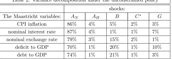
In order to understand nature of the optimal policy we investigate how the optimal policy responds to the shocks. Based on variance decomposition of the Maastricht variables (presented inT able2) we choose to analyze the impulse responses to a nontraded productivity shock.
Table 2: Variance decomposition under the unconstrained policy
shocks:
The Maastricht variables: AN AH B C G
CPI in‡ation 86% 4% 5% 2% 3%
nominal interest rate 87% 4% 1% 1% 7%
nominal exchange rate 79% 3% 15% 2% 1%
de…cit to GDP 70% 1% 20% 1% 10%
debt to GDP 74% 1% 21% 1% 3%
Similarly to Lipi´nska (2008), monetary instrument of the optimal policy - the nominal interest rate decreases in response to a positive nontraded productivity shock. This stabilizes the de‡ationary pressures in the domestic nontraded sector and at the same time supports increase in aggregate output. As a result, the nominal exchange rate depreciates (in accordance with the uncovered interest rate parity condition). Interestingly, …scal component of the policy is characterized by a countercyclical behaviour. Such a behaviour of taxes has its origin in a speci…c structure of the economy, i.e. openness and two domestic sectors. First of all, as already studied by Benigno and De Paoli (2006) an open economy nature of the economy gives the optimal policy maker an incentive to use taxes in the countercyclical way thanks to existence of terms of trade externality.27 By setting higher taxes in
the sector where the shock occurred the optimal policy maker can engineer a welfare-improving real exchange rate appreciation. Secondly, two sector structure creates important trade-o¤s for the optimal policy maker. This trade-o¤ was already studied by Gali and Monacelli (2005) in a model of monetary union, where monetary and …scal policy are set optimally under full coordination. In their model, each country’s …scal authority faces a trade-o¤ between stabilization of domestic in‡ation as opposed to output and …scal gap. Since the cost of in‡ation is higher than of the changes in distortionary taxation the optimal policy maker allows for ‡uctuations in the …scal instruments.28 As a result, in our model revenue taxes in the nontraded sector rise in order to
2 5This additional element is a bit ad-hoc although it is motivated by an idea of model stationarization by Schmitt-Grohe and
Uribe (2003). Alternatively, if one assumes that government debt is denominated in foreign currencies introduction of portfolio adjustment costs (presented by Schmitt-Grohe and Uribe (2003)) would also stationarize the model.
2 6For the purposes of sensitivity analysis we also present the results for
d= 10 5and also for the unconstrained policy d= 0: 2 7This incentive is present under an assumption of the substitutability between home and foreign goods.
2 8Notice however that on the contrary to our model Gali and Monacelli (2005) study a demand side …scal instrument, i.e.
[image:18.612.155.485.294.407.2]stabilize the nontraded output and de‡ation in the nontraded sector. At the same time, revenue taxes in the home traded sector decrease to stabilize the home traded output and in‡ationary pressures in this sector.
Consequently, as in Gali and Monacelli (2005) domestic in‡ation stabilizes. Moreover, output increases in both domestic sectors. Finally, since the overall tax revenues rise de…cit to GDP and debt to GDP decrease.
[F igure(1) about here]
Let us investigate now which Maastricht criteria are not satis…ed by the optimal policy. Under the optimal policy means of all the variables are zero so the reinterpreted Maastricht criteria can be reduced to the constraints that set upper bounds on the variances of the Maastricht variables, i.e.:
d
var(bt) (K 1)B2 (53)
d
var(Rbt) (K 1)CR2 (54)
d
var(Sbt) (K 1)D2S (55)
d
var(dfbt) (K 1)Fdf2 (56)
wherevard(xt)with xt=bt;Rbt;Sbt;dfbtis de…ned by (35).
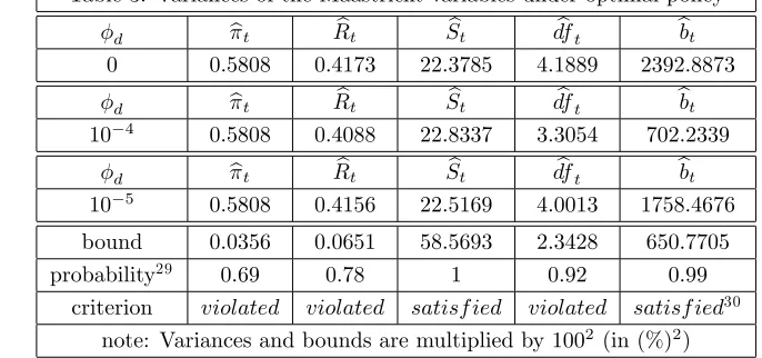
[image:19.612.138.481.470.631.2]In the table below (T able 3) we present the variances of the Maastricht variables together with the upper bounds implied by the Maastricht criteria. We also show variance of debt to GDP and a respective bound for this variables in accordance with the limit set out in the Maastricht Treaty. Let us note that although variances of debt and de…cit to GDP ratio do depend on the chosen value of the coe¢cient dvariances of other Maastricht variables do not.
Table 3: Variances of the Maastricht variables under optimal policy
d bt Rbt Sbt dfbt bbt
0 0.5808 0.4173 22.3785 4.1889 2392.8873
d bt Rbt Sbt dfbt bbt
10 4 0.5808 0.4088 22.8337 3.3054 702.2339
d bt Rbt Sbt dfbt bbt
10 5 0.5808 0.4156 22.5169 4.0013 1758.4676 bound 0.0356 0.0651 58.5693 2.3428 650.7705
probability29 0.69 0.78 1 0.92 0.99
criterion violated violated satisf ied violated satisf ied30
note: Variances and bounds are multiplied by1002 (in (%)2)
2 9Since debt follows a near nonstationary and also very persistent process we perform a Monte Carlo simulation exercise in which
we simulate our model forT = 50periods and repeat this simulationJ= 1000times. Based on this, we can calculate the average probabilities, for each of the Maastricht variables, of compliance with the criteria. We assume that a given criterion is not satis…ed if the probability for a given variable is lower than 95% (which is in accordance with the parameterk).
The optimal unconstrained policy does not satisfy three of the Maastricht criteria: the CPI in‡ation criterion, the nominal interest rate criterion and the de…cit to GDP criterion. As a result, the loss function of optimal policy that satis…es the Maastricht criteria has to have some additional elements.
6.3
The constrained optimal policy
6.3.1 The optimal policy constrained by monetary criteria
Now we analyze the policy constrained only by monetary criteria: CPI in‡ation rate and the nominal interest rate. In particular, we examine whether in the presence of the monetary criteria …scal policy can act as an additional stabilization tool.
First, we present parameters of the loss function associated with this constrained policy. The loss function takes the following form:
e
Lmt =Lst+
1
2 (
T
bt)2+
1
2 R(R
T Rb
t)2 (57)
where >0; R >0and T <0; RT <0:Similarly to the policy constrained only by the …scal criterion,
values of parameters( ; R; T; RT)can be obtained from the solution to the minimization problem of the loss
functionLs
t constrained by structural equations and also the monetary constraints. T able4provides the speci…c
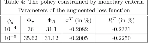
values for all the parameters for two di¤erent values of the penalty coe¢cient on debt ‡uctuations. It appears that values of the parameters of the constrained policy by monetary criteria do not depend to a great extent on the degree of debt stabilization ( d). Importantly, values of the penalty coe¢cients on the nominal interest
rate and CPI in‡ation rate are of the same magnitude as the penalty coe¢cients of the domestic in‡ation rates in the original loss function. Deterministic component of the constrained policy tells us that the policy maker constrained by monetary criteria should target CPI in‡ation rate and the nominal interest rate that are0:8%
[image:20.612.195.441.460.533.2]p:a:lower than in the countries of reference.
Table 4: The policy constrained by monetary criteria Parameters of the augmented loss function
d R T (in %) RT (in %)
10 4 36 31.1 -0.2082 -0.2331
10 5 35.62 31.12 -0.2005 -0.2250
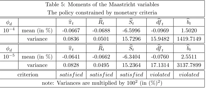
to shocks. Subsequently, surplus to GDP is characterized by much higher variance and so does de…cit to GDP and debt to GDP.
Table 5: Moments of the Maastricht variables The policy constrained by monetary criteria
d bt Rbt Sbt dfbt bbt
10 4 mean (in %) -0.0667 -0.0688 -6.5996 -0.0969 1.5020
variance 0.0836 0.0501 15.7296 15.9482 1419.7149
d bt Rbt Sbt dfbt bbt
10 5 mean (in %) -0.0641 -0.0662 -6.3404 -0.0760 2.5511
variance 0.0828 0.0495 15.2364 17.1314 3137.7899
criterion satisf ied satisf ied satisf ied violated violated
note: Variances are multiplied by1002 (in (%)2)
Third, we analyze how the policy constrained by monetary criteria di¤ers from the optimal unconstrained policy in the stabilization process of an economy hit by a shock. We choose the shock that explains the most of variability of the Maastricht variables (seeT able2 on variance decomposition).
[F igure(3) about here]
The policy constrained by monetary criteria aims at stabilizing CPI in‡ation and restricts the nominal interest rate movements. Accordingly, the monetary policy increases nominal interest rate on impact. Thanks to this, nominal exchange rate depreciates by less dampening the in‡ationary impact of the import sector on the aggregate CPI. However such a contractionary behaviour of the monetary policy leads to stronger de‡ationary pressures in the domestic sector. The domestic de‡ation is partly stabilized by the …scal component of the constrained policy which is more countercyclical than the unconstrained policy, i.e. revenue taxes rise in both domestic sectors. This leads to a much stronger decrease in de…cit to GDP, debt to GDP and also dampened increase in domestic aggregate output in comparison with the unconstrained policy.
6.3.2 The optimal policy constrained by …scal criterion
Let us now present the constrained policy by the …scal criterion: de…cit to GDP criterion. We concentrate on how the …scal criteria a¤ect the ability of …scal policy to stabilize business cycle ‡uctuations. The loss function of the policy constrained by the de…cit to GDP criterion can be represented in the following way:
e
Lft =Ls
t+
1
2 df(dfT dft)2 (58)
where Ls
t = Lt+ ddbt and df > 0 and dfT < 0: The solution to the minimization problem of the loss
functionLs
t constrained by structural equations and also the constraint on de…cit to GDP gives us values for
the parameters df and dfT: We present these values inT able 6 for two di¤erent values of the coe¢cient on
Table 6: The policy constrained by de…cit to GDP criterion Parameters of the augmented loss function
d df dfT (%)
10 4 0:0304 1:58
10 5 0:0219 6
Values of the penalty coe¢cient on the de…cit to GDP ‡uctuations are small in comparison with penalty coe¢cients associated with the variables present in the loss function. At the same time, deterministic component of the constrained policy involves targeting surplus to GDP equal to1:6%:The sensitivity analysis reveals that parameters of the augmented loss function do depend on the chosen value of d:However the general pattern of the constrained policy is the same. The goal of complying with the de…cit to GDP criterion is achieved rather through deterministic component than the stabilization one.
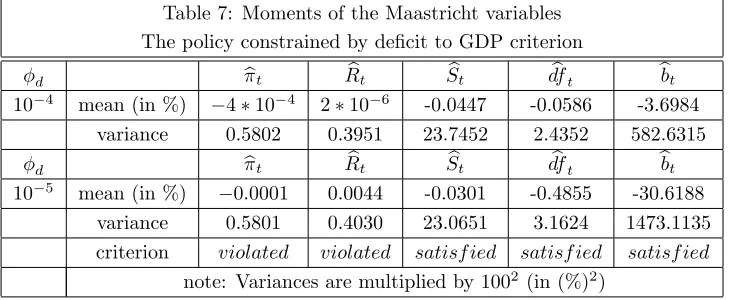
Let us now check how the optimal policy constrained by de…cit to GDP criterion a¤ects compliance of the monetary criteria. InT able7we present the means and variances of all the Maastricht variables and also report whether each of the criteria is satis…ed (based on the inequalities (30)–(33)).
Table 7: Moments of the Maastricht variables The policy constrained by de…cit to GDP criterion
d bt Rbt Sbt dfbt bbt
10 4 mean (in %) 4 10 4 2 10 6 -0.0447 -0.0586 -3.6984 variance 0:5802 0:3951 23.7452 2:4352 582.6315
d bt Rbt Sbt dfbt bbt
10 5 mean (in %) 0:0001 0.0044 -0.0301 -0.4855 -30.6188
variance 0.5801 0.4030 23.0651 3.1624 1473.1135 criterion violated violated satisf ied satisf ied satisf ied
note: Variances are multiplied by1002 (in (%)2)
Although the e¤ects of a nonzero target for de…cit to GDP are quantitatively small we can see that a negative target for de…cit to GDP results in smaller discounted means of in‡ation, the nominal exchange rate and (by de…nition) also of debt to GDP. On the other hand, mean of the nominal interest rate (and also of aggregate output) increases as a result of the smaller means of revenue taxes (to be seen later when analyzing the impulse responses). Moreover, a smaller variance in the de…cit to GDP triggers smaller variances of the CPI in‡ation and the nominal interest rate. At the same time, variance of the nominal exchange rate increases (this is in line with a higher variance of aggregate output - to be later seen in the analysis of impulse responses).
In order to understand how the nature of the policy constrained by de…cit to GDP criterion di¤ers from the optimal unconstrained policy, we analyze how both policies respond to the shocks. As previously, we concentrate on impulse responses to a positive nontraded productivity shock.
[F igure(2) about here]
[image:22.612.137.502.325.475.2]policy component of the constrained policy is more contractionary than under the unconstrained policy. Nominal interest rate decreases by less on impact than under the unconstrained policy leading to a smaller decline in debt interest payments. As a result, de…cit to GDP decreases by less (surplus to GDP increases by less) and so does the debt to GDP. Moreover, the constrained policy is characterized by higher on impact nominal exchange rate depreciation than under the unconstrained policy. This is consistent with a slightly higher aggregate output (due to lower taxes). Finally, a higher nominal exchange rate depreciation leads to a higher on impact CPI in‡ation under the constrained policy.
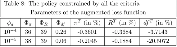
6.3.3 The optimal policy constrained by all the Maastricht criteria
Having analyzed the impact of monetary and …scal criteria separately on the optimal policy, we turn to the characterization of the optimal policy that complies at the same time with the monetary and …scal criteria. In particular, we analyze which criteria: put more constraints on the optimal policy.
Similarly to previous sections, we present the parameters of such a policy, its moments and also response of the constrained policy to a positive nontraded productivity shock. Apart from that, we analyze welfare losses associated with the constrained policy and compare them with the loss of the optimal unconstrained policy. We also analyze which criteria: monetary or …scal contribute the most to the generated loss under the constrained policy.
The loss function of the policy constrained by …scal criterion: de…cit to GDP and the monetary criteria: CPI in‡ation and the nominal interest rate can be represented in the following form:
e
Lt=Lst+
1
2 (
T
bt)2+
1
2 R(R
T Rb t)2+
1
2 df(df
T df
t)2 (59)
where >0; R>0; df >0and T <0; RT <0; dfT <0:Values of the parameters of such a constrained
policy are obtained from the solution to the minimization problem of the loss function(Ls
t)constrained by the
structural equations and …scal and monetary criteria. As can be seen inT able8; penalty coe¢cients of all the variables of interest are higher than under the policies that are only constrained by …scal or monetary criteria. This feature re‡ects con‡icting targets of each of the constrained stabilization policies. As far as targets are concerned we detect signi…cant di¤erences for de…cit to GDP. As previously, we observe that although targets of de…cit to GDP and debt do depend on the chosen value of the coe¢cient d values of the targets of the
[image:23.612.176.461.532.608.2]monetary variables are not so much sensitive.
Table 8: The policy constrained by all the criteria Parameters of the augmented loss function
d R df T (in %) RT (in %) dfT (in %)
10 4 36 39 0.26 -0.3601 -0.3684 -3.7143
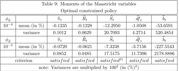
10 5 38 39 0.06 -0.2045 -0.1884 -20.5072
InT able9we show moments of the Maastricht variables under the optimal policy constrained by monetary