Monopoly, Diversification through Adjacent Technologies, and Market Structure

Munich Personal RePEc Archive

Monopoly, Diversification through

Adjacent Technologies, and Market

Structure

Karaaslan, Mehmet E.

Işık University

1 October 2007

Online at

https://mpra.ub.uni-muenchen.de/7607/

Monopoly, Diversification through Adjacent Technologies,

and Market Structure

Mehmet E. Karaaslan

Isik University,

Faculty of Economics and Administrative Sciences, Sile Istanbul, 34980, Turkey

E-mail:memin@isikun.edu.tr

WWW home page:http://iibf.isikun.edu.tr

Abstract. The theoretical literature on technological competition has been mostly concerned with various aspects of innovative activity in a single mar-ket. By contrast, this paper studies the adoption of a sequence of product innovations in two markets characterized by a common technology base, and illustrates the effects of technological rivalry and preemption. Under a perfect information scenario, it is shown in a two incumbent model that if the innovation is drastic (total replacement of the old product), under certain conditions the fear of being preempted by the entrant forces the firms to diversify their product lines by adopting the innovations across each other’s markets. On the other hand, with non-drastic innovation (partial re-placement of the old product), it is more likely for the firms to diversify in their own product lines. Out of a class of equilibria characterized un-der non-drastic innovation, one is optimal in which innovations are adopted in the firms’ own markets. In the Pareto inferior equilibria, the firms ei-ther adopt innovations in each oei-ther’s market so that incumbency changes hands or jointly adopt both innovations in two separate product lines. Perfect Bayesian equilibria are characterized under an asymmetric information sce-nario where one of the firms is assumed to have complete information about the relevant costs of adopting an innovation in a separate product line. If the priors are based on pessimism, it is more often subject to exploitation by the informed firm leading to pooling equilibrium, while optimistism more often leads to diversification and to a competitive market structure in both product lines under a separating equilibrium. In all the cases considered, both innovations are adopted, and in most cases they are adopted by the high cost entrant. The former is socially desirable, but the latter is not. More competitiveness necessarily implies wasteful expenditure by the high cost firm. Lack of competitiveness and technological rivalry, on the other hand, imply that maximum product diversity may not be achieved. Keywords: tehnological rivalry, preemption, adoption of innovations, up-grading.

1. Introduction

market, it is almost certain that successive generations of upgraded versions with additional features will follow. As successive innovations generate rich product di-versity in the marketplace, it is always those firms at the cutting edge of technology which persistently carry out R&D activity for upgrading and “perfecting” the prod-uct, to achieve or maintain a monopoly position that will skim the profits until a next generation product comes along. This, simply, is the Schumpeterian innovative process.

We also observe in the “sequences of innovations” process that the upgrad-ing products will incorporate developments and/or findupgrad-ings of other product lines. While the underlying basic science required for a certain product innovation in a sequence of innovations could be very distinct from another innovation in a sepa-rate product line, it is becoming more likely that both product lines will share and contain the latest developments in some other technology and R&D base. Examples of these innovations and ‘add ons’ are all around us in cell phones, digital cameras, pocket pcs (PDAs), portable audio, video, digital imaging, communiation and stor-age devices. We observe many other examples of technological convergence in recent product generations especially in consumer electronics industries that is fuelled by the shrinking size of semiconductors .

I call the process in which composite technologies are increasingly embodied in generations of successive product innovations “technological convergence”. For example, cameras and camcorders use the same optics technology base. As they become more ‘sophisticated’ we observe that microprocessors of various sort are being incorporated to increase their functions and capacity. VHS recorders followed by 8 mm camcorders which also function as players, are now being replaced with digital recording and digital cameras which all can be incorporated in a cell phone with still and movie camera features. This sequence illustrates the common practice of leading firms of technologically progressive industries diversifying their R&D base further from their initially established technological base, as the composite technology required to upgrade a product becomes increasingly diverse.

This aspect of increasing product diversification under technological convergence has been ignored in the theoretical R&D and innovation adoption literature. Ac-cording to the prevailing theory firms may diversify into multiple product lines in re-sponse to excess capacity of productive factors (Montgomery and Wernerfelt, 1988). Accordingly, technological scope economies embodied in the excess heterogeneous productive factors create incentives to diversify1_{. In this article I attempt to explain}

firm diversification based on strategic adoption of innovations and add on features. Specifically, I explore the effects of the strategic adoption of product innovations by separate monopolists on market structure. I conjecture that most innovations which are subject to strategic behavior on the part of the innovating or adopting firms are part of a sequence of innovations in a product line. By a “sequence of innovations” in a product line I mean a series of either qualitative (better functioning and/or more

1

durable, etc.)2_{or quantitative (with additional functions/features incorporated)}3 _,

or some combination of both, upgrading opportunities. Rosen calls this process‘add-on innovatiprocess‘add-ons,’ (Rosen, 1991) but emphasises process‘add-only the case of process innovatiprocess‘add-ons. I follow Reinganum’s (Reinganum, 1985) market driven definition of innovation, but focus only on the product innovations instead of process innovations. Reinganum calls an innovation “drastic” if the innovator becomes a monopolist in the post adoption market. I, instead, call an innovation drastic if the add-on technology that upgrades the product makes the previous version obsolete by completely replacing it. Hence, a drastic innovation that embodies an add-on technology can be adopted by more than one firm. Consider the audio cassette tapes that almost totally re-placed the earlier betamax tapes, or the color TV that in most part rere-placed the black and white TV which in turn will possibly be replaced by HDTV in the very near future. These are new products that use the same basic technology with the old products. Similarly, a non-drastic innovation that partly replaces the old prod-uct – in the sense of a demand shift – can make the adopting firm a monopolist in the upgraded product market. Sony, for example, used to be a monopoly in the ‘recordable CD player’ market in the early 1990’s while the ‘CD player’ market was competitive. Consequently, a single success does not mean that the successful firm reaps monopoly profits forever (Reinganum, 1985). Rather, monopoly profits are earned only until the next, better innovation is developed and successfully adopted by the innovative firm and is accepted by the consumers4

2

Examples to the idea of qualitative upgrading could be found in the innovations in pharmaceuticals industry (in headache pills and cold medicine market it would imply rapid effectiveness and fewer side effects), synthetics industry (in cassette/video tapes and photograph films/digital imagemaking industry it would imply higher resolution), and high definition TV (better picture quality).

3

Examples to the quantitative upgrading would be certain products in consumer elec-tronics industry (calculators, computers, DVD players, cell phones, cameras, and etc).

4

The idea of the models used in this paper is that each monopolist must choose either to preserve its own monopoly position by adopting an innovation in its prod-uct line or to challenge the incumbent monopolist in another market by adopting an innovation in that product line. Special features of the models arise from the differential costs in adopting innovations across separate product lines. Namely, if there is a product innovation to be adopted, any firm that is considering adoption is a potential entrant to the market which the adoption is expected to create. With the assumption that innovations have no patent protection and are common knowl-edge to all firms, the cost of entry to the potential market is the cost of adopting the innovation. I maintain that the cost of adoption would not be identical across existing firms considering undertaking R&D for this purpose. Unless the innovation is an original idea unrelated to any existing product market, the costs of adoption will be different across firms, depending on how suitable each firm’s R&D program is to the requirements of adoption and how close its existing product line(s) is to the innovation under consideration. If the innovation is part of a sequence of inno-vations in a product line, the existing firm(s) in that product line would have a cost advantage in adoption. This is due to the experience in production and learning by doing in R&D as well as the already established and technologically substitutable cospecialized assets which they might simply alter for the new product. This paper seeks to shed light on the importance of cost advantages in adoption and answers the question why firms sometimes give up these advantages and choose to enter a new market.

The theoretical literature on R&D and the adoption of new technologies has been concerned with different aspects of innovative activity in a single market. One main body of research concentrates on the incentives and the process of bring-ing about inventions. To cite a few representative contributions among many, see: (Dasgupta and Stiglitz, 1980), (Dasgupta, 1986) on the industrial structure, uncer-tainty and the speed of R&D; (Harris and Vickers, 1985), on patent races and per-sistence of monopoly (Gilbert and Newberry, 1982); and on licensing of innovations and network externalities (Katz and Shapiro, 1985).

Another line of research concentrates on the strategic aspects of the adoption of new technologies, again among the many, the following are few representative contributions: on the timing of innovation and the diffusion of new technology

(Reinganum, 1981); on rent dissipation (Fudenberg and Tirole, 1985, 1987); on market entry dynamics (Smirnov and Wait, 2007); on the sequence of innovations and industry evolution (Reinganum, 1985), (Vickers, 1986); and on divisionalization (Schwartz and Thompson, 1986).

The main effects governing R&D and technological rivalry have been mostly ana-lyzed using game theoretical tools. The results, with a few exceptions (Arrow, 1962), generally support Schumpeter’s (Schumpeter, 1942) thesis that monopoly situations and innovativeness are intimately related. Nevertheless, the focus has been on a sin-gle market where an incumbent and an entrant engage in some sort of technological supremacy game mostly for process innovations rather than product innovations.

The existing literature does not address the issues related to substitutability in basic science and technology when separate firms engage in strategic competition in R&D. That literature mostly treats an innovation as a generic idea unrelated to any existing product line. Furthermore, models which consider sequences of inno-vations (Reinganum, 1985), (Mclean and Riordan, 1989)) do not establish the links between the sequence of innovations in separate product lines. These links can be quite important depending on the technology and R&D base which is common knowledge to the firms sharing it. The knowledge of the common technology and R&D base enables firms considering adoption of an innovation to recognize their po-tential challengers and their relative strengths and weaknesses. The empirical work of Cockburn and Henderson (1994) is an exception to this. The authors studied research activity by 10 major pharmaceutical companies in pursuit of the discovery of ethical drugs over 17 years and have found the presence of complementarities and spillovers between firms leading to multiple prizes out of a single R&D race. Hence, the authors show that the implication of the early theoretical ”racing” models are inconsistent with the causal facts and their empirical results.

Of the product innovations mentioned earlier, I first focus on the drastic inno-vations using the perfect information framework. Following the general structure of the basic model, strategic competition for the new product markets are analyzed under three separate cases. Using the competitive payoffs as a benchmark for classi-fying the type of innovations, the Nash equilibrium points (NEP) are characterized. Under high cost drastic innovations the model is shown to represent a prisoner’s dilemma situation where the firms only diversify, and hence switch their product lines. Under medium cost drastic innovations where pure strategy equilibrium does not exist, the mixed strategy equilibrium is characterized using a theorem. Follow-ing this, an example of mixed strategy equilibrium is presented which satisfies the criteria developed in the theorem.

2. Drastic Innovation Under Perfect Information

The following model assumes that there is no uncertainty related with post-adoption market conditions, and that a firm will successfully replace the old product if it adopts the innovation in that product line. Total replacement of the old product by making it obsolete is the ’drastic’ nature of the innovation. Secondly, it is assumed that all agents involved in the innovative process are perfectly informed about all payoff relevant parameters of all agents, and that this perfect information is common knowledge to all agents.5

Consider a two period game with two identical firms sharing the closest technol-ogy base in two separate markets. In period one, assume that two separate products are exclusively and successfully produced by the two firms. Let firm 1 be the mo-nopolist producing a1, and firm 2 be the monopolist producing a2. Both firms are

earning monopoly profits equal toπm_{. Firm 1, (2) can adopt a}′

1, (a′2) (the innovation

in its own product line) with a costc , and it can adopt a′

2, (a′1) (the innovation in

the other firm’s product line) with a costkcwherek >1, or adopt both innovations with a cost c(1 +k), where c(1 +k)≤πm_.

Firms can adopt four strategies in this non-cooperative, one shot game : adopt a′

1, adopt a′2, adopt botha′1& a′2, or adopt neither (stick with the existing product).

If they both adopt either a′

1 or a′2 they compete as Cournot duopolists in that

product line. Both firms earn Cournot profits equal toπc _{in this case. If only one}

firm adopts, it totally replaces the old product and becomes a monopolist earning monopoly profits equal to πm _{in that product line. Symmetry assumptions about}

period two profits and markets are restrictive but they focus the analysis on the role that incumbency plays in the adoption of new technologies. The assumption of equal profits in period one is also due to the same consideration. I introduce the following notation:

πm

ij: Per period monopoly profit of firmi in marketj ,{i,j = 1,2}

πc

ij: Per period Cournot profit of firm i in market j, if it shares the market with

the other firm.

ciu: Cost to firmiof upgrading its product line by adopting the innovation in own

marketi

c_id: Cost to firmi of diversifying into another market by adopting the innovation in marketj .

Following restrictions are consistent with our discussion above.

πm

ij > π1jc +πc2j ; πmij > πi1c +πi2c ; πc1d=π2dc (i)

cid=kciu , k >1 (ii)

πm

ij ≥cid ∀ i, j= 1,2 (iii)

Inequalities in equation (i) are a general result of Cournot model (Tirole, 1988), (Shy, 2000), and symmetry assumptions imposed on the firms and markets. Accord-ingly, monopoly profits in one market strictly exceed the total Cournot profits of both firms in that market. Alternately, the total of Cournot profits any firm can

5

earn in two separate markets is strictly less than monopoly profits it can earn in one market.

Equation (ii) states that the cost of adopting the innovation in any firm’s product line is strictly less than the cost of adopting the innovation in the other product line. In other words, diversifying is costlier than upgrading.

Equation (iii) imposes the restriction that payoffs to being a monopolist in any market are non-negative. If the inequality holds for the incumbent but not for the entrant, lacking any threat of entry, there would be no incentive for the incumbent to adopt the innovation in its own product line since it would simply be replacing itself as a monopolist. Thus the restriction eliminates only a trivial case.

The following notation is introduced to simplify the characterization and man-ageability of the model. Accordingly the pure strategies for firm i are denoted by:

si1: no action (stick with the existing product)

si2: upgrade only (adopt the innovation in own product line)

si3: diversify only (adopt the innovation in the competitor’s product line)

si4: upgrade and diversify (adopt both innovations)

Payoffs of the game are defined in terms of period 2 flow profits minus the cost of adoption. I use the following notation to denote the payoffs:

πm

i : monopoly profits of firmi in own marketi when no upgrading and entry has

taken place

Vm

id : monopoly profits in other marketj , (requires i to adopt an innovation that

allows it to diversify into marketj)

Vm

iu : monopoly profits in own marketi , (requires i to adopt an innovation that

allows it to upgrade its product)

Vc

iu : profits in own marketi when product is upgraded but competitor has

diver-sified and entered marketi

Vc

id : profits in other marketj wheni has diversified but incumbent has upgraded.

πc

ii : profits of firm i in own market i when no upgrading has taken place and

entrant has diversified in the upgraded product, (by definition,πc

ii = 0 for

drastic innovations)

For example, suppose in period two, firm 1 decides to stick with its existing product a1, and firm 2 diversifies by adopting a′1. Since by definition of drastic

innovations, a′

1totally replaces the market for a1, firm 1 (the incumbent) is preyed

upon by firm 2 (the entrant) in its own market. Firm 1 becomes a monopolist in both product lines producing a′

1 and a2. Thus, the payoffs to firm 1 and 2 respectively

are{0, πm

22+ Vm2d}.

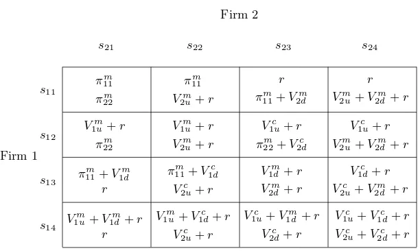
Firm 1

Firm 2

s21 s22 s23 s24

s11 πm 11 πm 22 πm 11 Vm 2u 0

π22m+V2md

0

V2mu+V2md

s12 Vm 1u πm 22 Vm 1u Vm 2u

V1cu

πm

22+V2cd

V1cu

Vm

2u+V2md

s13 π

m

11+V1md

0

πm11+V

c

1d

Vc

2u

V1md

V2md

V1cd

V2cu+V2md

s14 V

m

1u+V1md

0

V1mu+V1cd

V2cu

V1cu+V1md

V2cd

V1cu+V1cd

V2cu+V2cd

Table 1.Strategic game with drastic innovations under perfect information.

The solution concept employed is payoff dominance. This method assumes eco-nomic agents behave rationally and it is common knowledge to the players that each player would play rationally. When players consider any two strategies , they would compare their payoffs in each cell of the corresponding strategies of the normal form. If in all pairwise comparisons one strategy yields payoffs that are strictly greater than the other, at least in one comparison and are equal in all the others, then it is said that the first strategy weakly dominates the second one. After players eliminate all dominated strategies, the game is then played on the remaining undominated strategies. Finally, Nash equilibrium point(s) (NEP) are searched.

Nash equilibrium points (NEP’s) are strategy combinationss∗

1i, s∗2i, that are

best replies to each other, such that E1(s∗1, s∗2,) = max_s11

i

E1(s1, s∗2)and E2(s∗1, s∗2) =

max

s2i

E2(s∗1, s2) where (si, sj) is the combination of thei’ th strategy of firm 1 and

j’ th strategy of firm 2.

Differences in the cost of adopting an innovation for the incumbent and the entrant result in three separate cases to consider.

Case 1 : πc

ij≤ciu<cid, ∀i,j = 1,2{Viuc ≤0, Vidc <0}

Case 2 : ciu<cid≤πcij, ∀i,j = 1,2{Viuc >0, Vidc ≥0}

Case 3 : ciu< πijc <cid, ∀i,j = 1,2{Viuc >0, Vidc <0}

2.1. High Cost Drastic Innovations

The conditions used in classifying an innovation as high-cost are (i) diversifying with an upgraded product is not profitable (Vc

id < 0), and (ii) competition in

an upgraded product is not profitable either (Vc

iu≤0). Next, the payoff dominant

strategies -if they exist- are searched for, and after eliminating all possible dominated strategies the NEP’s in pure strategies are found. If pure strategy NEP’s do not exist, equilibrium in mixed strategies is characterized.

Lemma 1. Supposeπc

ij≤ciu<cid,∀i,j = 1,2{Viuc ≤0 ;Vidc <0}. Then,

(a)π1(s1, s)≥π1(s2, s) andπ2(s, s1)≥π2(s, s2) ∀s

(b)π1(s3, s)≥π1(s4, s)andπ2(s, s3)≥π2(s, s4) ∀s,

whereπi(sk, sl)isi’ s payoff when firm 1 chooses skand firm 2 chooses sl.

(proof: see the appendix for all proofs not given in the main body of the text.)

Proposition 1. Under drastic innovation whereπc

ij ≤ iu < cid, the NEP is the

strategy combination{s3, s3} with payoffs (V1dm;V2dm). Thus the monopolists cross

over and diversify into the other firm’s market.

Remark 1. Since innovations are drastic, there is a one-hundred percent replace-ment of the incumbent’s product line. From the firms’ point of view (s1, s1) may be

the “better” outcome; yet it is not self-enforcing and therefore not “stable”. They are facing a classic ’prisoner’s dilemma’ situation. Thus, each incumbent is pre-empted by the other monopolist, so that the monopolists switch markets. Although both innovations are adopted, the outcome is sub-optimal not only from the firms’ viewpoint but also from a social standpoint since high cost entrants rather than the low cost incumbents are undertaking the adoption of innovations.

Example: πm

i = 10, ciu = 4, cid= 5 , Vium = 6, Vidm= 5, Viuc =−1, Vidc =

−2. It is a simple exercise to plug in the values above into the generalized normal form given in table 1 and see that{s3, s3} is the NEP with corresponding payoffs

of (5,5). High Cost Drastic Innovations:πc

ij<ciu < cid (Viuc <0 ; Vidc <0)

Example:πm

i = 10 ,ciu= 4 , cid= 5 ,Vium=6 , Vidm=5 ,V c

iu=-1 , Viuc =-2 .

Firm 1

Firm 2

s21 s22 s23 s24

s11 10 , 10 10 , 6 0 ,15 0 ,11

s12 6 , 10 6 , 6 −1 , 8 −1 , 4

s13 15 , 0 8 ,−1 5 , 5∗ −2 , 4

s14 11 , 0 4 ,−1 4 , 2 −3 ,−3

Example

2.2. Low Cost Drastic Innovations

I say the innovations are low cost when both the diversification to compete with an upgraded product, and the competition in an upgraded product are profitable (

Vc

iu>0;Vidc ≥0). In other words, no matter what the rival firm does, undertaking

an innovation is profitable for both the entrant firm and the incumbent firm.

Lemma 2. Supposeciu<cid≤πcij ,∀i, j= 1,2,{Viuc >0 ,Vidc ≥0}. Then

(a)π1(s3, s)≥π1(s1, s) ,π2(s, s3)≥π2(s, s1) ∀s

(b)π1(s4, s)≥π1(s2, s),π2(s, s4)≥π2(s, s2) ∀s

whereπi(sk, sl)isi’ s payoff when firm 1 chooses sk and firm 2 chooses sl.

Proposition 2. Under drastic innovation where ciu <cid ≤πcij , the NEP is the

strategy combination {s4, s4} with payoffs (V1uc +V1dc ; V2uc +V2dc). Thus, the

mo-nopolists upgrade and diversify in both product lines by adopting both innovations.

Remark 2. Since competitive payoffs following a joint adoption of an innovation are greater than or equal to zero in each market, the monopolists upgrade and di-versify in order to avoid being preempted by the entrant. The outcome is clearly pro competitive even though the monopolists spend greater portion of their resources for a product innovation in which they have a comparative disadvantage. Their monopoly positions are replaced with Cournot Competition. Notice that in the re-duced game the firms face a prisoner’s dilemma situation as in the previous case of high cost innovations.

Example: πm

i = 10, ciu= 2 , cid = 3 Vium = 8, Vidm= 7 , Viuc = 2 , Vidc = 1

It is a simple exercise to plug in the values above into the generalized normal form given in table 1 and see that {s4, s4} is the only NEP with corresponding payoffs

of (3,3).

Firm 1

Firm 2

s21 s22 s23 s24

s11 10 , 10 10 , 8 0 , 17 0 , 15

s12 8 , 10 8 , 8 2 , 11 2 , 9

s13 17 , 0 11 , 2 7 , 7 1 , 9

s14 15 , 0 9 , 2 9 , 1 3 , 3∗

Example

Fig. 2.Low cost drastic innovations.

2.3. Medium Cost Drastic Innovations

Innovations are classified as medium cost under the following assumptions. The first is the condition that diversifying to compete with an upgraded product is not profitable, i.e., Vc

product is profitable, i.e.,Vc

iu>0. These conditions. together with case 1 and case

2 exhaust the payoff spectrum under all possible strategy combinations chosen by the incumbent and the entrant. The idea of ’medium cost’ embodies within it the concept of comparative advantage of being established in a product line. All else being equal, if the incumbent has to compete with an entrant in a product that it has upgraded, the incumbent will prevail and prey upon the entrant. Knowing its comparative disadvantage, the entrant will enter only if can secure a monopoly on the product line it is diversifying into. On the other hand, the incumbent monopolist is reasoning that if it does not adopt the innovation and upgrade its product, it will be preyed upon by a successful entrant -no matter how much a cost disadvantage exists. Because of the drastic nature of the innovation, no matter who adopts it, the existing product will be obsolete.

It is easy to see that there are not any payoff dominated strategies that can be eliminated to simplify the solution. It is also straightforward to verify that there are no NEP in pure strategies in this game either. Therefore, the NEP’s has to be characterized using mixed strategies.

Letα= (α1, α2, α3, α4) denote firm 1’s mixed strategy and β = (β1, β2, β3, β4)

denote firm 2’s mixed strategy. Then, write the expected payoffs for each firm as follows:

E1(α, β) =α1(β1+β2)π11m+α2{(β1+β2)V

m

1u+ (β3+β4)V

c

1u}

+α3{(β1+β2)πm11+ (β1+β3)V

m

1d+ (β2+β4)V

c

1d}

+α4{(β1+β2)V

m

1u+ (β1+β3)V

m

1d+ (β2+β4)V

c

1d+ (β3+β4)V

c

1u}

E2(α, β) =β1(α1+α2)π22m+β2{(α1+α2)V

m

2u+ (α3+α4)V

c

2u}

+β3{(α1+α2)π22m+ (α1+α3)V

m

2d+ (α2+α4)V

c

2d}

+β4{(α1+α2)V

m

2u+ (α1+α3)V

m

2d+ (α2+α4)V

c

2d+ (α3+α4)V

c

2u}

Proposition 3. Assume Vium< πmii,Viuc >0,Vidc <0 ∀ i= 1,2. Then, any NEP

in mixed strategies must satisfy the following :

(β1+β3)V1dm+ (β2+β4)V1dc = 0 (1)

(α1+α3)V

m

2d+ (α2+α4)V

c

2d= 0 (2)

Proposition 4. Under the assumptions of Proposition 3, any NEP in mixed strate-gies must satisfy the following :

(α1+α2)π22m = (α1+α2)V2um+ (α3+α4)V

c

2u (3)

(β1+β2)πm11= (β1+β2)V1um+ (β3+β4)V

c

Theorem 1. ∀πc

ij andπiic such that,ciu< πijc<cid,V

m

iu < πmii {i,j=1,2} holds, the

set of all mixed strategy NEP’s satisfies:

(β1+β3)V1dm+ (β2+β4)V1dc = 0

(β1+β2)(πm11−V1um)−(β3+β4)V1uc = 0

β1+β2+β3+β4= 1, βi≥0

(α1+α3)V

m

2d+ (α2+α4)V

c

2d= 0

(α1+α2)(πm22−V2um)−(α3+α4)V

c

2u= 0

α1+α2+α3+α4= 1, αi ≥0

whereαandβ are firm 1’s and firm 2’s mixed strategies respectively.

Proof of Theorem 1: This theorem is a consequence of the definition of medium cost drastic innovations, and of Propositions 3 and 4.

The corresponding expected payoffs are:

E1(α, β) =α1(β1+β2)πm11+α2{(β1+β2)V1um+ (β3+β4)V

c

1u}+α3(β1+β2)πm11

+α4{(β1+β2)V1um+ (β3+β4)V

c

1u}

E2(α, β) =β1(α1+α2)πm22+β2{(α1+α2)V

m

2u+ (α3+α4)V

c

2u}+β3(α1+α2)π22m

+β4{(α1+α2)V

m

2u+ (α3+α4)V

c

2u}.

Simplifying the equations inNEP* we obtain:

(α1+α2) =

V2uc

πm

22−V2um+V

c

2u

(5)

(α3+α4) =

πm 22−V

m

2u

πm 22−V

c

2u

(6)

(α1+α3) =

V_2dc Vm

2d −V

c

2d

(7)

(α2+α4) =

V_2dm Vm

2d −V

c

2d

Remark 3. From (5) we note that the lower is the cost of upgrading , the more likely is that the incumbent will stay in own product line and upgrade its product . Similarly, from (6) we note that the higher is the cost of upgrading , the more likely is that the entrant will either cross over to a separate product line or diversify into both product lines.

In the following numerical example I find the range of individual probabilities for mixed strategy NEP’s.

Example : πm

ij=10, πijc=4 ∀ i,j = 1,2 ; ciu=3, cid=5 Vium = 7 , Vidm =

5, Vc

iu= 1, Vidc =−1

The following table depicts the normal form representation of this example.

Firm 1

Firm 2

s21 s22 s23 s24

s11 10 , 10 10 , 7 0 , 15 0 , 12

s12 7 , 10 7 , 7 1 , 9 1 , 6

s13 15 , 0 9 , 1 5 , 5 −1 , 6

s14 12 , 0 6 , 1 6 ,−1 0 , 0

Example

Fig. 3.Medium cost drastic innovations.

Let A1,...,A4 be the expected payoffs firm 1 will receive if firm 2 plays the mixed strategies (β1, ..., β4) and let B1,...,B4 be the expected payoffs firm 2 will receive if

firm 1 plays the mixed strategies (α1, ..., α4). Then, using the payoffs in the example,

the following linear equation systems are set up for firm 1 and firm 2 respectively.

A1=π1(s1, β) = 10β1+ 10β2

A2=π1(s2, β) = 7β1+ 7β2+β3+β4

A3=π1(s3, β) = 15β1+ 9β2+ 5β3−β4

A4=π1(s4, β) = 12β1+ 6β2+ 6β3

B1=π2(α, s1) = 10α1+ 10α2

B2=π2(α, s2) = 7α1+ 7α2+α3+α4

B3=π2(α, s3) = 15α1+ 9α2+ 5α3−α4

B4=π2(α, s4) = 12α1+ 6α2+ 6α3

Equating A1=A4 , A2=A4 , A3=A4 and using the constraint that the sum of the probabilities of random strategies is equal to oneP4

i=1βi = 1, I proceed to find

2β1−4β2+ 6β3= 0 (i)

5β1−β2+ 5β3−β4= 0 (ii)

−3β1−3β2+β3+β4= 0 (iii)

β1+β2+β3+β4= 0 (iv)

We also want to place the restriction thatβ1, β2, β3, β4≥0 . Note that (i) - (ii)

= (iii). Therefore, we eliminate (i). From (iii) we have,

(β1+β2) =(β3+β4)

3 .

Substituting this into (iv) we obtain,

(β3+β4)

3 + (β3+β4) = 1 or,

(β3+β4) =

3 4

= π

m 11−V

m

1u

πm 11−V

m

1u+V

c

1u

(9)

It follows that,

(β1+β2) = 1

4 = V c 1u πm 11−V

m

1u+V

c

1u

. (10)

From (ii) we have,

5(β1+β3) = (β2+β4).

Substituting this into (iv) we obtain,

β1+β3+ 5(β1+β3) = 1

or,

(β1+β3) =

1 6

= − V

c

1d

Vm

1d−V

c

1d

. (11)

It follows that,

(β2+β4) =

5 6 = V m 1d Vm

1d−V

c

1d

. (12)

We have shown that equations (9) through (12) satisfy equations (5) through (8) respectively. It is also immediate that, from equations (9) through (12) we can write the following conditions:

0≤β1≤

1

6 , 0≤β2≤ 1

4 , 0≤β3≤ 1

6 , 0≤β4≤ 3

Hence, it is seen that, in this example, any interior solution for the mixed strategy equilibria must satisfy (13). Simulations show that one solution that satisfies the non-negativity constraints are the followingβi values:β1= 0, β2= 0.25, β3 =

0.17, β4= 0.58.

2.4. Summary of Results

If the innovation is drastic, i.e., that it would totally replace the existing product in that product line, then the firms would: (i) diversify into the incumbent’s product line only and in the process switch markets as monopolists if and only ifπc

ij≤ciu<

cid; (ii) upgrade in own product line and diversify into the competitor’s product line

and compete as Cournot competitors by adopting the innovations in both product lines if and only if ciu <cid < πijc : and (iii) use a mixed strategy equilibrium in

deciding which innovation(s) they would adopt if and only if, ciu< πijc <cid.

Under the first type of equilibrium with “drastic” innovation we find that firms diversify their product lines by crossing over markets and totally replace the in-cumbents, if payoffs from the competitive outcome are non-positive (i.e., if the innovations are high cost) for both the entrant and for the incumbent. This type of equilibrium where the monopolists switch markets develops as a dominant ‘defen-sive’ strategy because under drastic innovation firms do not undertake adoptions in their own product lines, since it would only mean replacing themselves as incum-bents. It can be concluded that, because competition reduces profits, each firm’s incentive to become a monopolist is greater than its incentive to become a duopolist by jointly adopting the high cost innovation.

Under the second type of equilibrium, firms upgrade products not only in their own product line but also in the incumbent’s product line. This type of total di-versification arises when competitive payoffs from diversifying into the competitor’s product line is non-negative, i.e., when the innovations are low cost.

We also observe that under some boundary values of cost of adoption and Cournot profits, firms may use mixed strategy equilibrium. We get mixed strat-egy equilibrium with drastic innovation if the profits from Cournot competition in any market strictly cover the cost of adoption for the incumbent, but are strictly less than the cost of adoption for the entrant, i.e., if the innovations are medium cost. Both innovations are adopted, however, either through switching of incumbency, or by the incumbent itself, or by joint adoption in both product lines, as demonstrated with a numerical example.

3. Non-drastic Innovation Under Perfect Information

With non-drastic innovation (or partial replacement of the old market) we mean that successful adoption of the innovation: (i) suppresses the demand for the old product but does not make it completely obsolete, and (ii) generates new demand so that the total demand in that product line is growing. In this model, up to 4 product markets (2 in each product line) can coexist in the second period. If both innovations are adopted exclusively, either by the incumbent or by the entrant, the payoff that can be earned from each new product market is Vm

i The costs of

adoption, suppressed inVm

i , are ci where cid>ciu, for alli=1,2.

The profits incumbent firms earn from their respective old markets, if the inno-vation is adopted, are denoted by a parameter ri, where 0<ri ≤πim. ri = 0 would

imply a drastic innovation where the old product market is totally replaced by the new one. On the other hand, ri =πim implies that adoption of the innovation has

no effect on the old product market. While this is an extreme case of non-drastic innovation, no replacement indicates that the two products are possibly unrelated or not considered to be on the same product line on the demand side.

I modify the notation used for drastic innovations to simplify the characteri-zation of the model.

The pure strategies for firmi are denoted by: The pure strategies of firmi are denoted by:

si1 : no action (stick with the existing product)

si2 : upgrade only (adopt the innovation in own product line, and continue

produc-ing the old product ifr >0 .

si3 : diversify only (adopt the innovation in the competitor’s product line)

si4 : upgrade and diversify (adopt both innovations, and continue producing the

old product ifr >0.

Payoffs to firmi are denoted by:

πm

i : pre-innovation monopoly profits in own marketi (when firmi sticks with its

old product and no upgrading has taken place )

πc

ij : Cournot profits of firm i when both firms jointly adopt the innovation in

marketj

ri : post-innovation monopoly profits the incumbent earns from its old product

marketi, (requires upgrading by the incumbent and/or diversification through adoption of an innovation by the competitor into marketi)

Vm

id : monopoly profits in other market j, (requires i to adopt an innovation that

allows it to diversify into marketj, but the incumbent does not upgrade)

Vm

iu : profits from having the monopoly of the new product in own marketi,

(re-quiresi to adopt an innovation that allows it to upgrade its product)

Vc

iu : profits from the new product in own marketi when product is upgraded but

competitor has diversified and entered marketi

Vc

id : profits in other marketj whenihas diversified by adopting an innovation but

incumbent has upgraded.

πmij >2π c

ij ∀ i, j= 1,2 (i)

cid > ciu ∀ i, j= 1,2 (ii)

Vm iu, V

m

id >0 ∀ i, j= 1,2 (iii)

0≤r≤πm. (iv)

Recall that (i) states that the total of Cournot profits any firm can earn in two separate markets is strictly less than the monopoly profits it can earn in a single market. Hence, monopoly is always a preferred status by both firms.

Equation (ii) states that the cost of adopting the innovation in any firm’s prod-uct line is strictly less than the cost of adopting the innovation in the competitor’s product line capturing the idea of comparative cost advantage obtained by being an established firm in a product line. It implies6_Vm

iu > V m id, andV

c iu> V

c

id ∀i= 1,2

meaning’upgrading to keep monopoly is better than diversifying to obtain monopoly’ for the former, and ’divesifying to compete with an upgraded product is less prof-itable than upgrading to compete with an entrant that has diversified in the upgraded product’ for the latter.

Equation (iii) imposes the restriction that payoffs to being a monopolist in any market are non-negative. If not, it is either too costly for both the entrant and the incumbent to earn positive profits following an adoption, or it is too costly only for the entrant to earn positive profits even if it became a monopolist in the incumbent’s product line. It implies that πm _{> c}

iu, cid ∀ i = 1,2. If the

inequality holds for the incumbent (Vm

iu > 0), but not for the entrant (Vidm < 0),

then, under drastic innovation (r= 0) there would be no reason for the incumbent to adopt the innovation in its own product line since it would be replacing itself as a monopolist (Vm

iu =πm). Thus, this restriction not only eliminates a trivial case but

also captures the idea of technological closeness and rivalry. When (iii)holds, firms find themselves within the technological boundaries of one another; hence, they see themselves as potential challengers and entrants in the incumbent’s product line.

Note that (ii) and (iii) together imply the following: First, upgrading to obtain monopoly is better than diversifying into another market to obtain monopoly,Vm

iu >

Vm

id ∀i= 1,2.

Second, diversifying to compete with an upgraded product is less profitable than upgrading to compete with an entrant that has diversified in the upgraded product,

Vc

iu> Vidc ∀i= 1,2.

Inequality (iv) captures the degree of replacement of the old product market by the adopted innovation. A drastic innovation where the old product market is totally replaced by the new one will be denoted byr= 0. On the other hand,r=πm

implies that adoption of the innovation has no effect on the old product market since the incumbent can earn the same amount of profits from its old product market. While this is an extreme case of drastic innovation, no replacement indicates that the two products are possibly unrelated.

6

However, it should be noted that Eq.(ii) does not imply eitherc1u> c2u, orc1d> c2d

Finally, note that using Equation (iv), together with (ii) and (iii) we require:

Vm

id +r > π

m _{∀i= 1,2 & 0≤r≤π}m_.

Hence, for a drastic innovation where r = 0, we require that Vm

iu, Vidm > π m_.

This defines the lower bound for profits so that the firms would not be worse off as monopolists if they considered upgrading and/or diversifying their product lines. I assume equal replacement in the two product lines, i.e., r1 =r2, without loss of

generality, to simplify the notation, as this does not change the results. AssumeVm

iu+ ri> πmi as a proxy that the total demand following adoption of an

innovation in a product line is growing7_{Next assumeV}m

iu > Vidmupgrading to obtain

a monopoly is better than diversifying into another market to obtain monopoly. Finally, assumeVc

iu> Vidc, diversifying to compete with an upgraded product is less

profitable than upgrading to compete with an entrant that has diversified in the upgraded product.

Table 2 depicts the normal form representation of the general model. For exam-ple, if the firms exclusively adopt the innovations in their own product lines, the strategy combination for firm 1 and firm 2 would be denoted by (s2, s2), respectively.

In this case, each firm maintains its monopoly position for both the old and the new markets in its product line. This strategy yields payoffs ofπi(s2, s2) =Vium+ ri

and it is the maximum that can be earned as a monopolist in a single product line. The strategy combination (s4, s4) means that the firms both adopt the innovations

in their product lines and across product lines while continuing to produce their original products. Thus, the firms become Cournot competitors in the new product markets and maintain their monopoly positions in the old product markets which is suppressed by the new products. In this case, payoffs to firm 1 and firm 2, in respective order, are as follows.

π1(s4, s4) =V1uc +V1dc + r1;π2(s4, s4) =V2uc +V2dc + r2.

Similar to the case of drastic innovations, differences in the cost of upgrading and diversification result in three separate cases to consider under this scenario also.

Case 1 : πc

ij<ciu<cid, ∀i,j = 1,2{Viuc <0 ; Vidc <0}

Case 2 : ciu<cid< πcij, ∀i,j = 1,2{Viuc >0 ; VidcA >0}

Case 3 : ciu≤πijc ≤cid, ∀i,j = 1,2{Viuc ≥0 ; Vidc ≤0}

I label the above cases as high cost, low cost and medium cost respectively.

3.1. High Cost Non-drastic Innovations

If competitive payoffs to both the incumbent firm and the entrant firm following a joint adoption of an innovation in any market are strictly negative, I call them high cost innovations:8 (Viuc <0 ; Vidc <0) .

7

Vium+ ri=πm_i , implies the innovation is non-drastic, but it has simply generated new

demand and revenues enough to compensate exactly for the cost of its adoption.

8

Recall that high cost innovations were defined as (Vc iu≤0 ; V

c

id<0) earlier. I ignore the

Firm 1

Firm 2

s21 s22 s23 s24

s11

πm11

πm22

πm11

V2mu+r

r π11m+V2md

r V2mu+V2md +r

s12

V1mu+r

πm

22

V1mu+r

Vm

2u+r

V1cu+r

πm22+V2cd

V1cu+r

V2mu+V2md +r

s13 π

m

11+V1md

r

πm

11+V1cd

Vc

2u+r

V1md +r

Vm

2d +r

V1cd+r

Vc

2u+V2md+r

s14 V

m

1u+V1md+r

r

Vm

1u+V1cd+r

V2cu+r

Vc

1u+V1md+r

Vc

2d+r

Vc

1u+V1cd+r

Vc

2u+V2cd+r

Table 2.Strategic game with non-drastic innovations under perfect information.

Lemma 3. Supposeπc

ij<ciu<cid, (Viuc , Vidc <0) i = j. Then, (a)π1(s1, s4)> π1(s, s4)andπ2(s1, s4)> π2(s1, s)∀ s. (b)π1(s2, s2)> π1(s, s2)andπ2(s2, s2)> π2(s2, s)∀ s. (c)π1(s3, s3)> π1(s, s3)andπ2(s3, s3)> π2(s3, s)∀ s. (d)π1(s4, s1)> π1(s, s1)andπ2(s4, s1)> π2(s4, s)∀ s.

whereπi(sk, sl) is i”s payoff when firm 1 choosessk and firm 2 chooses sl.

Proposition 5. Under high-cost non-drastic innovation whereπc

ij<ciu<cid, the

pure strategy NEP’s are the strategy combinations {s1, s4}, {s1, s2}, {s3, s3}, and

{s4, s1}with payoffs(r1; V2um+V2dm+ r2),(V1um+ r1; V2um+ r2),(V1dm+ r1; V2dm+ r2),

and(Vm

1u+V1dm+ r1; r2)respectively.

Remark 4. Under two of the four equilibria, and , we observe a passive incumbent and an aggressive entrant. The entrant monopolist diversifies across both its own product line and the entrant’s product line, whereas the incumbent sticks with the old product and is partly preyed upon and replaced by the aggressive entrant. In the other two equilibria, and , both firms are actively involved in diversification and specialization process. In the former equilibrium, firms stay in their own market and upgrade in their own product lines. In the latter equilibrium, they diversify only in the incumbent’s product line; and in this process of switching, they partly replace the incumbent and are partly replaced by the entrant in their old markets.

Example:πm

i = 10, ciu = 4, cid = 5, Vium = 6, Vidm= 5 , Viuc =−1, Vidc =

−2 , r1 = r2 = 6. It is a fairly easy exercise to plug in the values above into the

{s4, s1} are the NEP’s with corresponding payoffs of (6,17), (12,12), (11,11), and

(17,6) respectively. r1and r2, are given equal values to make the payoffs symmetric.

Their equality is not necessary to drive the results.

Firm 1

Firm 2

s21 s22 s23 s24

s11 10 , 10 10 , 12 6 , 15 6 , 17∗

s12 12 , 10 12 , 12∗ 5 , 8 5 , 8

s13 15 , 6 8 , 5 11 , 11∗ 4 , 10

s14 17 , 6∗ 10 , 5 10 , 4 3 , 3

Example

Fig. 4.High cost non-drastic innovations.

Lemma 4. Supposeciu≤ πijc ∀ i, j= 1,2 {Viuc ≥0}. Then,

(a)π1(s2, s)≥π1(s1, s)andπ2(s, s2)≥π2(s, s1) ∀s

(b)π1(s4, s)≥π1(s3, s)andπ2(s, s4)≥π2(s, s3) ∀s

whereπi(sk, sl)is i’s payoff when firm 1 choosessk and firm 2 chooses sl.

3.2. Low Cost Non-drastic Innovations

I classify the non-drastic innovations as low cost if the competitive payoffs the entrant and the incumbent would separately earn in any market following a joint adoption of an innovation are strictly positive (Vc

iu>0, V c id >0).

Proposition 6. Under low-cost non-drastic innovations where ciu < cid < πijc,

{Vc

iu>0 ; Vidc >0}the NEP is the strategy combination{s4, s4}with payoffs(V c

1u+

Vc

1d+r1; V c

2u+ Vc2d+r2). Thus, each monopolist upgrades both in its own product

line and diversifies into the competitor’s product line while keeping the monopoly position in the old product market which is partly replaced by the innovation.

enters the incumbent’s market. Although the incumbent can not prevent entry, it avoids being partly preyed upon by the entrant, through upgrading its own product. Monopoly is replaced by competition in both of the new product markets since each monopolist both upgrades its own product line and diversifies into the competitor’s product line. However, each firm maintains the monopoly position in the old product market which, in part, is replaced by the innovation. The costly diversification may be justified for the presumably lower prices that would result under competition.

Example : πm

i = 10 , ciu = 2 , cid = 3 , Vium = 8 , Vidm = 7 , Viuc = 2 , Vidc =

1, r1= r2= 6.

Firm 1

Firm 2

s21 s22 s23 s24

s11 10 , 10 10 , 14 6 , 17 6 , 21

s12 14 , 10 14 , 14 8 , 11 8 , 15

s13 17 , 6 11 , 8 13 , 13 7 , 15

s14 21 , 6 15 , 8 15 , 7 9 , 9∗

Example

Fig. 5.Low cost non-drastic innovations.

When the above values are inserted into the generalized normal form given in table 2 we see that the NEP is{s4, s4}, and the corresponding payoffs are (9,9).

3.3. Medium Cost Non-drastic Innovations

Medium cost innovations are defined such that competition with an upgraded prod-uct is profitable (Vc

iu≥0) but diversifying to compete with an upgraded product is

not (Vc id≤0).

Proposition 7. Under medium-cost non-drastic innovation where ciu ≤ πijc ≤

cid {Viuc >0 ; Vcid>0}, the NEP is the strategy combination {s2, s2} with payoffs

(Vm_1u+r1; Vm2u+r2). Thus, the monopolists stay in their product lines and upgrade

Remark 6. Since innovations are non-drastic each firm stays as a monopolist in the old product market and also guarantees a non-negative payoff by upgrading its own product even if the competitor diversifies. On the other hand, diversifying yields a non-positive competitive payoff. Thus, each incumbent effectively prevents entry by adopting only those innovations in its own product line and maintains its monopoly position. This is the optimal outcome from both the firms’ and the soci-ety’s standpoint. Both innovations are undertaken by the low cost firms established in those product lines. The threat of an incumbent prevents costly diversification which is desirable. Yet, both innovations are adopted through low cost upgrading by the incumbent firms which maintain their monopoly positions in their respective product lines.

Example: πm

i = 10 , ciu = 3 , cid = 5 , Vium = 7 , Vidm = 5 , Viuc = 1 , Vidc =

−1, r1= r2= 6

Firm 1

Firm 2

s21 s22 s23 s24

s11 10 , 10 10 , 13 6 , 15 6 , 18

s12 13 , 10 13 , 13∗ 7 , 9 7 , 12

s13 15 , 6 9 , 7 11 , 11 5 , 12

s14 18 , 6 12 , 7 12 , 5 6 , 6

Example

Fig. 6.Medium cost non-drastic innovations.

A simple inspection upon plugging the values above into table 2 shows that (s2, s2) is the NEP, with the corresponding payoffs of (13,13).

3.4. Summary of Results

Multiple equilibria arises with non-drastic innovation if competitive payoffs of both the entrant and the incumbent are strictly negative (πc

ij<ciu <cid); in other

words if the innovations are high cost type. Under this scenario a multiplicity of best reply strategies for each monopolist range from adopting both innovations, to not adopting any of the innovations. Both innovations are adopted, however, under any of the possible Nash equilibria. An interesting point is that, under two of the four possible equilibria, we observe a passive incumbent and an aggressive entrant. The entrant monopolist diversifies across both its own product line and the entrant’s product line, whereas the incumbent sticks with the old product and is partly preyed upon and replaced by the aggressive entrant. In the other two multiple equilibria both firms are actively involved in diversification and specialization process. In one of the equilibrium, firms stay in their own market and diversify in their own product lines. In the other equilibrium, they diversify only in the incumbent’s product line; and in this process of switching, they partly replace the incumbent and are partly replaced by the entrant in their old markets.

Under the second type of equilibrium with low cost innovations, firms upgrade products not only in their own product line but also in the incumbent’s product line. This type of total diversification arises when competitive payoffs from diversifying into the competitor’s product line is non-negative (ciu < cid < πcij). This latter

result is obtained under both the drastic and non-drastic low cost innovations. Under the third type of Nash equilibrium, monopolists stay in their own markets and increase their specialization and upgrading of existing products. We get this result under Nash equilibrium with medium cost non-drastic innovations (ciu ≤

πc

ij ≤ cid), i.e., when the cost of diversifying in another product line exceeds the

flow profits of a possible competitive outcome.

The main tendency is that if the firms are facing non-drastic innovations, then, they would either upgrade in their own product lines only, or upgrade and diversify into both product lines. Unlike the case of drastic innovation, firms do have the incentive to upgrade their own products even without the technological rivalry. The existence of a potential threat of entry into the incumbent’s product line enhances the process of diversification and the firms might find themselves with excessive diversification across all possible product lines within their technological reach. The optimal outcome from both the society’s and the firms’ standpoints dictates that the firms adopt innovations in their own product lines since the same maximum product diversity could be achieved by the least cost monopolist. However, not only that this can not be enforced as a credible commitment, but it would also imply that the incumbents’ monopoly positions would have to remain unchallenged. Clearly, this process of strategic inventiveness is in accord with the Schumpeterian concept of “creative destruction”.

4. A Model of Innovation Adoption under Asymmetric Information

would enable the uninformed firm to form conjectures, update its prior beliefs and make assessments.

In this section I work with the non-drastic innovation case and consider the drastic innovation as a special case.(Refer to Table 2. for the generalized normal form game.)

Payoffs are as defined in the base model of section 3. I shall, however, suppress the first subscript of the above notation when writing the payoffs under different strategy combinations. For example, the payoff to firm 2 unders12ands22strategy

combinations will be denoted byπ2(s2, s2) =V2mu+r, and the strategy combination

(s4, s4) now means that the firms adopt the innovations both in their product lines

(upgrading) and across product lines (diversifying) while continuing to produce the old products. Thus, the firms become Cournot competitors in the new product markets and maintain their monopoly position in the -now suppressed-old product markets. In this case, the payoffs to firm 1 and firm 2, in respective order, are as follows:

π1(s4, s4) =V1cu+V c

2d+r

π2(s4, s4) =V2cu+V c

2d+r

Next, recall that there are types of the players determined by 3 possible cost structures defined with respect to the competitive payoffs of each firm. I identify each cost structure with a possible firm type, denoted by Nij(jthtype of firm i).

These firm types are given as follows:

(i) Ni1:Viuc ≤0, V c

id <0 (π c_≤c

iu < cid)

(ii) Ni2:Viuc >0, V c

id <0 (ciu< πc < cid)

(iii) Ni3:Viuc >0, Vidc ≥0 (ciu< cid≤πc)

From the incumbent’s point of view, the competitor’s type is an indicator of whether it is a low cost, medium cost, or a high cost entrant. From the entrant’s point of view, the incumbent’s type is an indicator of whether it would fight back to block entry, accommodate the entrant and share the new product market, or yield the monopoly position in its product line.

Suppose, firm 1 has private information about his own type and that of firm 2, but firm 2 does not.–throughout this paper we shall assume that firm 1 is the informed player, and first mover. Firm 1 observes both its own type (N1j) and its

competitor’s type (N2j).

Firm 2, on the other hand, knows only the adoption costs in its own product line,c2u , which enables it to conclude whetherV2cu≤0 orV2cu>0. If, in fact,c2uis

too high such thatVc

2u≤0, then it follows thatV2cu<0since by initial condition(ii)

we have c2u < c2d. This enables firm 2 to conclude that his type is (N21). Firm 2

does not need additional information to decide whether its type is (N21)or not.

When firm 2 is of type (N21), her best reply to the strategy played by firm 1

the informed player and has complete information about the types of both firms. This information advantage enables firm 1 to be the first mover regardless of his own type, and firm 2 accepts its leadership.

Lemma 5. For the uninformed firm, its best reply to s11is given as follows:

s24=b2(s11) ∀ N2j, j= 1,2,3.

Proof (of lemma). From Table 1 we immediately see that,

π2(s1, s4|N2j)−π2(s1, s3|N2j) = (V2mu+V2md +r)−πm+V2md)

=Vm

2u + r−π m_≥0

π2(s1, s4|N2j)−π2(s1, s2|N2j) = (V2mu+V m

2d +r)−(V m

2u+r)

=Vm

2u>0

π2(s1, s4|N2j)−π2(s1, s1|N2j) = (V2mu+V m

2d +r)−(π m₎

= (V2mu + r−π m

) +V2md >0 ⊓⊔

We denote firm 2’s best reply to the strategysplayed by firm 1 byb2(s):

b2(s) = arg max

s′

π2 π2(s, s′)

Then, a Stackelberg equilibrium is a pair of strategies (s∗_{, b}

2(s∗)) such that,

s∗= arg max

s π1(s

∗_{, b}

2(s∗)).

Next, the following lemma is used to construct normalized strategies of firm 2 as a function of her type,N2j

Lemma 6. For the uninformed firm, its best replies given that it knows its type, are given as follows:

(a) s22=b2(s12) if f N2=N21, N22

s24=b2(s12) if f N2=N23

(b) s23=b2(s13) if f N2=N21

(c) s21=b2(s14) if f N2=N21

s22=b2(s14) if f N2=N22

s24=b2(s14) if f N2=N23.

Table 3 summarizes firm 2’s best reply strategies as a function of her type and the corresponding payoffs to both firms.

F irm 1′_s

Leader Strategy

F irm2′_s

Best Reply

F irm 1′_s

P ayof f

F irm 2′_s

P ayof f

s1 s4 r V2mu+V2md +r

s2 s2, if V2cd<0

s4, if V2cd>0

Vm

1u+r

V1cu+r

Vm

2u+r

V2mu+V c

2d+r

s3 s3, if V2cu<0

s4, if V2cu≥0

V1mu+r

Vc

1d+r

V2md+r

Vc

2u+V2md+r

s4 s1, if V2cu<0, V2cd<0

s2, if V2cu>0, V2cd<0

s4, if V2cu>0, V2cd>0

Vm

1u+V1md+r

V1mu+V1cd+r

Vc

1u+V1cd+r

r V2cu+r

Vc

2u+V2cd+r.

Table 3.Stackelberg equilibria and payoffs under perfect information.

Lemma 7. For the informed firm, the following payoff dominance relationships hold if the uninformed firm is of typeN2J{J = 2,3}

(a)

(a) π1(s2, s2|N11)> π1(sk, s2|N11) ∀ k= 1,3,4

π1(s1, s4|N11)> π1(sk, s4|N11) ∀ k= 2,3,4

(b) π1(s2, s2|N12)> π1(s, s2|N12)

π1(s2, s4|N12)> π1(s, s4|N12)

(c) π1(s4, s2|N13)> π1(s, s2|N13)

4.1. Stackelberg Equilibria

It should be noted that only in the case where firm 1 leads by playing itss11strategy,

is firm 2’s best reply not a function of its type; i.e., firm 2 does not need to know its type to play its best reply strategy,s24. Consequently we can write the following

proposition.

Proposition 8. If firm 1 has perfect information, then (s4, s1) is a Stackelberg

equilibrium if and only if firm 2’s type isN21.

Proof (of proposition).

Proposition 8 can be easily proved by inspecting Table 2 :

If (s4, s1) is a Stackelberg equilibrium, then from the last part of table 3,s1 =

b2(s4) if V2cu >0,V1cd <0, i.e., firm 2 s type is N21. Conversely, suppose firm 2’s

type isN21..

Then, consider each strategy of firm 1:

s4=b2(s1)⇒π1(s1, b2(s1)) =r

s2=b2(s2)⇒π1(s2, b2(s2)) =V1mu+r

s3=b2(s3)⇒π1(s3, b2(s3)) =V1mu+r

s1=b2(s4)⇒π1(s4, b2(s4)) =V1mu+V1md +r

From this we see thats4= arg maxsπ1(s, b2(s)) ands1=b2(s4).

Thus, (s4, s1)is a Stackelberg equilibrium. ⊓⊔

Remark 7. Under (N11, N21), (N12, N21)and(N13, N21) the uninformed player can

deduce that it is a high cost firm without further information or signaling by firm 1, the informed player. Under the above states of the world, firm 2 need not know which type of a competitor (high cost/medium cost/low cost) it is facing. Firm 2’s best response solely depends on its own type,N21. Firm 1 benefits from its information

advantage only because it is the first mover. An interesting aspect of the NEP is that it is determined without any reference to the leader’s type. Firm 1 might be a high cost or medium cost firm(N₁₁orN12). But this is irrelevant for the particular

NEP obtained, as long as firm 1 is the first mover. Firm 1 uses the first mover advantage; it upgrades and diversifies to obtain monopoly position in both the old and the new product markets. Firm 2, on the other hand, continues to produce the old product and exploits the residual demand as a declining monopolist.

Proposition 9. The following strategy combinations obtain under the following states of the world9_{when firm 1 is the Stackelberg leader, and firm 2 is the follower.}

If(N11, N22), then the Stackelberg equilibrium is(s2, s2);

If(N12, N22), then the Stackelberg equilibrium is(s2, s2);

If(N13, N22), then the Stackelberg equilibrium is(s4, s2);

If(N11, N23), then the Stackelberg equilibrium is(s1, s4);

If(N12, N23), then the Stackelberg equilibrium is(s2, s4);

If(N13, N23), then the Stackelberg equilibrium is(s4, s4);

Proof. Analogous to the proof of Proposition 8 as it is seen from Table 3.

9

4.2. Perfect Bayesian Equilibrium with a medium/low cost follower The Solution Concept:

To firm 2, firm 2 is either typeN22or N23; firm 1 can be any of N11,N12,N13.

Being uninformed, firm 2 assigns prior probabilities Pr(N22) = φ, Pr(N23) =

1−φ; Pr(N11) =θ1; Pr(N12) =θ2; and Pr(N13) =θ3,φ≥0,θj ≥0,θ1+θ2+θ3=1

These prior beliefs are common knowledge, i.e., they are known to both firms. Firm 2 knows that firm 1 knows her prior beliefs, and firm 1knows that firm 2 knows that he knows her beliefs, and so on. Firm 2 has to update its beliefs after observing certain strategies played by firm 1.

Suppose for example, that firm 2 observess12 being played by firm 1. Her type

might be either N22 or N23. Seeing s12 should make firm 2 update the posterior

belief, Pr(N22|s12) . The natural method is to use Bayes’s rule, which shows how

to revise the prior belief in the light of data. It uses two pieces of information that firm 2 knows: the likelihood of seeing s12 given that the state of the world

is N22, Pr(s12|N22), and the likelihood ofs12 given that the state of the world

is, N23, Pr(s12|N23). Since there are only 2 alternatives to firm 2’s type, the

marginal likelihood of seeings12 as a result of one or another possible types of

firm 2, (N22or N23) is given by,

Pr(s12) = Pr(s12|N22) Pr(N22) + Pr(s12|N23) Pr(N23).

The probability that both the strategys12played and the state of the worldN22

occurs is:

Pr(s12, N22) = Pr(s12|N22) Pr(N22)

= Pr(N22|s12) Pr(s12)

Firm 2’s new belief -its posterior- is calculated using Pr(s12), which yields the

following Bayes Rule.

Pr(N22|s12) =

Pr(s12|N22) Pr(N22)

Pr(s12)

The term Bayesian equilibrium is used to refer to Nash equilibrium when players update their beliefs according to Bayes’s rule (Rasmussen, 1989). Perfect Bayesian equilibrium point (PBEP) is a Stackelberg equilibrium (s*,β2(s∗)) whereβ2(s∗)is

the Bayesian best reply to to s* such that ,

β2(s) = arg max

s′

π2Eπ2(s, s′)

s∗= arg max

s′

π1(s, β2(s))

4.3. Characterization of Equilibrium

Theorem 2. Under asymmetric, imperfect and incomplete information where firm 1 is the informed player and where the states of the world are (N1j, N2l), ∀ =

1,2,3, l = 2,3, the perfect Bayesian equilibrium points are the following strategy combinations:

(a) :(s1, s4)iff (−)(

Vc

2d|,N22)

(Vc

2d|,N23) ≤

θ2(1−φ)

(θ1+θ2)φ andN1=N11

(b) :(s2, s4) iff(−)(V

c

2d|,N22)

(Vc

2d|,N23) ≤

θ2(1−φ)

(θ1+θ2)φ andN1=N12

(c) :(s4, s4) iff(−)(V

c

2d|,N22)

(Vc

2d|,N23) ≤

(1−φ)

φ andN1=N13

(d) :(s2, s2)iff (−)(V

c

2d|,N22)

(Vc

2d|,N23) ≥

θ2(1−φ)

(θ1+θ2)φ andN1=N11, N12

(e) :(s4, s2) iff(−)(V

c

2d|,N22)

(Vc

2d|,N23) ≤

(1−φ)

φ andN1=N13

First, recall from weak dominance firm 2’s dominant strategies are

s22 and s24when it is either medium or low cost (see table 4.2). Hence, firm 1

effectively faces a normal form game of dimension (4x2) if firm 2 is of eitherN22or

N23 type (see Table 4. for the reduced normal form).

Firm 1

Firm 2

s22 s24

s11 πm11 , V2mu+r r , V2mu+V2md+r

s12 V1mu+r , V2mu+r V1cu+r , V2mu+V2md +r

s13 π11m+V1cd , V c

2u+r V1cd+r , V c

2u+V2md+r

s14 V1mu+V c

1d+r , V c

2u+r V c

1u+V c

1d+r , V c

2u+V c

2d+r

Table 4.Reduced strategic game with non-drastic innovations under imperfect informa-tion.

I assume that firm 1, being an informed player, will always strive to reach the Stackelberg equilibrium that corresponds with its observed state. This assumption allows us to derive firm 2’s conjectures of observing a strategys1kconditional on her

Lemma 8. For the uninformed firm the following conjectures hold.

(a) : P r(s11, N22) = 3

X

i=1

Pr(s11|N1i, N22) Pr(N1i)

= Pr(s11|N11, N22) Pr(N11) + Pr(s11|N12, N22) Pr(N12)

+ Pr(s11|N13, N22) Pr(N13)

= 0

Pr(s11, N23) = 3

X

i=1

Pr(s11|N1i, N23) Pr(N1i)

= Pr(s11|N11, N23) Pr(N11) + Pr(s11|N12, N23) Pr(N12)

+ Pr(s11|N13, N23) Pr(N13)

= Pr(N11) =θ1

(b) : Pr(s12, N22) = 3

X

i=1

Pr(s12|N1i, N22) Pr(N1i)

= Pr(s12|N11, N22) Pr(N11) + Pr(s12|N12, N22) Pr(N12)

+ Pr(s12|N13, N22) Pr(N13)

= Pr(N11) + Pr(N12) =θ1+θ2

Pr(s12, N23) = 3

X

i=1

Pr(s12|N1i, N23) Pr(N1i)

= Pr(s12|N11;N23) Pr(N11) + Pr(s12|N12, N23) Pr(N12)

+ Pr(s12|N13, N23) Pr(N13)

= Pr(N12) =θ2

(c) : Pr(s14, N22) = 3

X

i=1

Pr(s12|N1i, N22) Pr(N1i)

= Pr(s14|N11, N22) Pr(N11) + Pr(s14|N12, N22) Pr(N12)

+ Pr(s14|N13, N22) Pr(N13)

= Pr(N13) =θ3

Pr(s14, N23) = 3

X

i=1

Pr(s14|N1i, N23) Pr(N1i)

= Pr(s14|N11, N23) Pr(N11) + Pr(s14|N12, N23) Pr(N12)

+ Pr(s14|N13, N23) Pr(N13)

= Pr(N13) =θ3

Remark on Separating and Pooling Equilibria:

Suppose part(d)of Theorem 2 holds, so that firm 2’s best reply tos12iss22We

note that under (d)firm 1 can be either a high cost type or a medium cost type. Clearly, by deciding on a best reply of s22 under (d) firm 2 can not differentiate

From lemma 7(b), recall that a medium cost firm 1’s best reply to eithers22 or

s24 iss12. From lemma 7(a), also recall that a high cost type firm 1’s best reply to

s22is alsos12. This indicates that under(d)an informed high cost firm successfully

pretends that it is medium cost type. Under(d) we obtain a pooling equilibrium. Next, suppose(a)holds. Notice that (a)is a perfectly symmetric condition to (d). In this case, firm 2’s best reply to s12is s24 . But(a) holds only if firm 1 is

high cost type so that his best reply to s24 is s11. In this case, a high cost firm

1 is successfully differentiated from a medium cost one. Under (a) we obtain a separating equilibrium.

Rational Priors at a Boundary Payoff :Vc id = 0

Recall that a firm is defined as medium cost -typeNi2−ifV_iuc >0 andV_idc <0

hold; and it is defined as low cost-type Ni3− ifV_iuc > 0 and V_idc ≥0 hold. Hence,

note that the lower bounds of Vc

id under the two types are given by the following

equations:

(Vc

id |Ni2) =−cid

(Vc

id |Ni3) = 0

Corollary 1. Suppose the uninformed firm’s competitive payoff is given by,(Vc

id |N23) =

0. Then, a separating equilibrium is obtained if and only if the following priors hold: 1−φ= 1,and/orθ3= 1

Proof. Suppose firm 2 observess12. Then, from the proof of Theorem 2 part (b) we

note that firm 2’s best reply tos12 iss24if and only if:

0≤θ2(1−φ)(V2cd|N23) + (θ1+θ2)φ(V2cd|N22)

Substituting (Vc

2d|N23) = 0, into the above equation we obtain,

0≤(θ1+θ2)φ(V2cd |N11, N22). (14)

But, since (Vc

2d |N22)<0 then, we require eitherθ1+θ2= 0 , and/or φ=

0 for (14) to hold. Hence, it is easily seen that:

1−φ= 1,and/orθ3= 1. ⊓⊔

Remark 8. If (Vc

2d|N23) then from theorem 2(b) we require (14) to hold for a

separating equilibrium (s2, s4). But, it is immediate that if there is a slight deviation

in the priors so that the reverse inequality to (14) holds then, we obtain the condition in part(d) which gives s22 as a Bayesian best reply to s12. Therefore, a pooling

equilibrium shall be obtained under part (d). Obviously, firm 2 would prefer a separating equilibrium to a pooling equilibrium as opposed to firm 1 who would rather have a pooling equilibrium. This clearly requires (14) to hold, enabling firm 2 to derive the range of her rational priors as defined in the corollary.

4.4. A Proposed Equilibrium Using “Equally Likely” Assumption A reasonable way to form priors for firm 2 is to conjecture that her type beingN22