Munich Personal RePEc Archive
Panel Cointegration and the Monetary
Exchange Rate Model
Basher, Syed A. and Westerlund, Joakim
12 September 2008
Online at
https://mpra.ub.uni-muenchen.de/10453/
Panel Cointegration and the Monetary Exchange
Rate Model
∗Syed A. Basher† Joakim Westerlund‡
September 12, 2008
Abstract
This paper re-examines the validity of the monetary exchange rate model during the post-Bretton Woods era for 18 OECD countries. Our analysis simultaneously considers the presence of both cross-sectional dependence and multiple structural breaks, which have not received much attention in previous studies of the monetary model. The empiri-cal results indicate that the monetary model emerges only when the presence of structural breaks and cross-country dependence has been taken into account. Evidence is also pro-vided suggesting that the breaks in the monetary model can be derived from the underlying purchasing power parity relation.
JEL Classification: C32; C33; F31; F41.
Keywords: Monetary exchange rate model; Purchasing power parity; Panel cointegra-tion; Structural break; Cross-section dependence.
1
Introduction
Lately, there has been renewed interest in the monetary model of exchange rate determina-tion, which states that the nominal exchange rate between two countries is determined by their relative levels of money supply and output. The by far most scrutinized proposition of this model is that exchange rates, relative money supply and relative output should be nonstationary and cointegrated.
∗We thank one anonymous referee for helpful comments and suggestions. Westerlund is grateful for financial
support from the Jan Wallander and Tom Hedelius Foundation under research grant number W2006–0068:1. The views expressed here are those of the authors and do not reflect the official view of the Qatar Central Bank. The usual disclaimer applies.
†Department of Economic Policies, Qatar Central Bank. E-mail:
‡Corresponding author: Department of Economics, Lund University, P. O. Box 7082, S-220 07, Lund,
Despite its strong theoretical appeal, however, the empirical success of the monetary model on an individual country-by-country basis has been rather limited, to say the least. For instance, Sarantis (1994) examines whether the monetary model holds for a collection of four countries between 1973 and 1990, and is unable to reject the null hypothesis of no cointegration. Recently, Rapach and Wohar (2002) employ annual data over the period 1880 to 1995 for 14 industrialized countries, and find that although there are some evidence of cointegration for eight of the countries, for the remaining six, there are no such evidence.
Thus, the empirical performance of the monetary model on an individual country-by-country basis has not been very convincing. But as Taylor and Taylor (2004) point out, time series results of this kind should not be taken too seriously, as the failure to reject the null hypothesis of no cointegration is more likely to reflect the low power of the tests employed rather than the failure of the monetary model.
One way to increase the power of such tests is to use not just one time series but a panel of multiple series. The panel data framework not only provides more data, which is a prerequisite for any sound empirical work, but also increases the power and accuracy of conventional time series unit root and cointegration tests, see Breitung and Pesaran (2008) for a recent overview of the literature. Two of the earliest studies within this field are those of Groen (2000) and Mark and Sul (2001). Groen (2000) employs a panel of quarterly data covering 14 OECD countries between 1973Q1 and 1994Q4. He finds evidence of cointegration for his G10 and full samples for both United States dollar and German mark numeraire currencies. Mark and Sul (2001) employ quarterly data for 18 countries spanning the period 1973Q1 to 1997Q1. They also find evidence of a cointegrating relationship consistent with the monetary model, regardless of the choice of numeraire currency considered. Hence, based on these pieces of evidence, the panel approach seems very promising indeed.
to fulfill the restrictions of the monetary model, which can very well explain the findings of Mark and Sul (2001).
Another shortcoming of the early panel studies mentioned above is that they are based on the assumption of cross-section independence among the countries in the panel. This as-sumption is problematic in general, and it is violated almost surely in the current application, as the use of a common numeraire country makes the remaining countries correlated.1
Yet another example of the restrictiveness of earlier studies is that the possibility of structural breaks is almost always ignored, which is likely to be particularly relevant when testing the monetary model because of different exchange rate regimes. It is a well-known fact that erro-neously omitted breaks can cause deceptive inference in time series testing, and it is expected to materialize in the panel context too. The effects of structural breaks do not disappear simply because one uses panel data.
In this paper, we simultaneously consider heterogeneity, cross-sectional dependence and structural breaks, which have not received much attention in previous panel based studies of the monetary exchange rate model. We accomplish this by applying two recently developed panel tests to the same data used by Mark and Sul (2001). To test the order of integration of the variables, we apply the panel stationarity test developed by Carrion-i-Silvestre et al. (2005), which is flexible enough to account for a large amount of heterogeneity, cross-section dependence and multiple unknown structural breaks. As a test for cointegration, we apply the test of Westerlund (2005), which can be seen as a residual-based version of the Carrion-i-Silvestre et al. (2005) test. Our results indicate that there is little evidence in favor of the monetary model when the analysis does not account for the effects of cross-country dependence and structural breaks. This conclusion is reversed when these features are taken into account. In an attempt to bring some light on the origin of the estimated structural breaks, we take a closer look at the purchasing power parity (PPP) relationship, which is one of the fundamental building blocks of the monetary model. Numerous studies have documented the presence of breaks in the PPP relation during the recent float era considered in this paper.2
Here, we follow Hegwood and Papell (1998) and permit for the possibility of structural breaks in both the level and trend of the PPP relation for each country. The results show that most
1
Indeed, as O’Connell (1998) notes, exchange rates constructed for instance using the United States as the numeraire country contains two common components, namely the variation in the value of the dollar and the variation in the corresponding price index. These two common components can be interpreted as common shocks affecting all exchange rates in the panel.
2
of the breaks in the monetary model can be attributed to breaks in the underlying PPP relation.
The rest of the paper is organized as follows. Section 2 briefly outlines the monetary model, while Section 3 discusses the econometric methodology. Section 4 presents the empirical results. Section 5 concludes.
2
The monetary exchange rate model
We focus our attention to a slightly modified version of the monetary model adopted by Groen (2002). Consider a panel comprised of t = 1, ..., T time series observations on i = 1, ..., N countries. The United States is treated as the reference country and is henceforth denoted by an asterisk. The monetary model is based on three important assumptions. The first assumption is that the following real money demand relation holds for all countries
mit−pit = ηi+φiyit−γiiit+vit, (1)
wheremit,pit,yitandiitare the logarithm of money supply, aggregate price level, real income
and nominal interest rate, respectively. The parametersφi andγi are the income and interest
rate elasticities, respectively, and ηi is a country specific intercept. The disturbance vit is
modelled as stationary and mean zero.
The second assumption is that the following version of PPP holds for each country
pit = µij+τijt+p∗t +sit+eit, (2)
where j = 1, ..., Mi + 1, p∗t is the logarithm of the United States aggregate price index, sit
is the logarithm of the nominal exchange rate between the domestic country and the United States, andeit is a mean zero stationary disturbance. Moreover, as in Hegwood and Papell
(1998), and Papell and Prodan (2006), we allow the country specific intercept and trend terms, here denoted by µij and τij, respectively, to vary over time. In particular, we allow
for the possibility of Mi structural breaks, or Mi+ 1 regimes, as indicated by the index j.
Thus, there areMi+ 1 regimes for each countryiwith thejth regime running formTij−1 to
Tij time series observations. In the terminology of Hegwood and Papell (1998), and Papell
depreciation rather than by discrete mean jumps. In addition, besides its better ability to explain the observed data, the allowance of the trend makes the model robust against possible Balassa-Samuelson effects.3
Now, by combining equations (1) and (2), we obtain the following solution for the nominal exchange rate
sit = αij+τijt+ (mit−m∗t)−φi(yit−y∗t) +γi(iit−i∗t) +uit, (3)
whereαij =η∗−ηi−µij and uit=vt∗−vit−eit. The final assumption is that the following
uncovered interest parity condition holds
Et(∆sit+1) = (iit−i∗t), (4)
where the operators ∆ andEt signify the first difference and the expectation conditional on
the information set available at timet, respectively. By direct substitution of (4) into (3), it is not difficult to see that
sit = αij+τijt+ (mit−m∗t)−φi(yit−y∗t) +wit, (5)
wherewit =γiEt(∆sit+1) +uit should be stationary since Et(∆sit+1) anduit are stationary
by construction. Therefore, since both empirical and theoretical work suggest that exchange rates, relative money supply and output are nonstationary, the monetary model necessi-tates thatsit is cointegrated with (mit−m∗t) and (yit−y∗t) forming the cointegrating vector
(1, −φi)′.4
3
Econometric methodology
In this section, we briefly describe the panel stationary test of Carrion-i-Silvestre et al. (2005) and the panel cointegration test of Westerlund (2005). We begin by considering the simple case when the countries are assumed to be independent, and then we continue to explain how
3
The Balassa-Samuelson effect embodies the idea that divergent international productivity levels can, via their effect on wages and home good prices, lead to permanent deviations from the no trend version of PPP. The argument is based on the fact that if PPP holds for traded goods, then productivity differentials between countries determine the domestic relative prices of non-tradables, leading in the long run to trend deviations from PPP.
4
the bootstrap procedure can be used to obtain valid tests when the members of the panel are dependent.
3.1 The tests
We begin by considering the cointegration test. As mentioned in the previous section, when exchange rates, relative money supply and relative output are nonstationary, the monetary model requires these variables to be cointegrated. To this end, consider the following empirical specification of our theoretical model
sit = αij +τijt+βi(mit−m∗t) +φi(yit−y∗t) +wit, (6)
whereβi and φi are country specific slope parameters that are assumed to be constant over
time, while αij and τij are again country specific intercept and trend parameters that are
subject toMi structural breaks. The errorwit is assumed to be generated as wit=git+εit,
where
git = git−1+ρiεit
with εit having a mean zero and stationary distribution that is independent across i. The
fact thatεit is only assumed to be stationary means that it can be both heteroskedastic and
serially correlated. That is, not only is the cointegration vector permitted to differ across both regimes and countries, the long-run variance ofεitis also permitted to vary freely across
countries. The assumption thatεit is independent acrossi is restrictive but will be relaxed
later on.
The essential insight that underlies this error structure is that if ρi is zero, git vanishes
under the assumption of zero initiation, in which case (6) is a cointegrated regression, asεitis
stationary by assumption. In other words, the value ofρi can be used to determine whether
Westerlund (2005), who develops a panel Lagrange multiplier test for cointegration that allows for multiple structural breaks.
The null hypothesis of interest is that all the countries in the panel are cointegrated, while the alternative is that there is a non-vanishing fraction of countries that are not cointegrated. This testing problem can be formulated in terms ofρiasH0 :ρi = 0 for alli, versusH1:ρi 6= 0
fori= 1, ..., N1 andρi= 0 fori=N1+1, ..., N, whereN1 is such that NN1 →0 asN1, N → ∞.
The Lagrange multiplier test statistic for this particular null hypothesis is given by
Z(M) = 1 N
N
X
i=1
MXi+1
j=1
Tij
X
t=Tij−1+1
S2
it
(Tij−Tij−1)2bσi2
,
where Sit = Pts=Tij−1+1wbst, wbit is the regression residual obtained by using any efficient
estimator of the cointegration vector such as the fully modified least squares estimator of Phillips and Hansen (1990), and σb2
i is the usual Newey and West (1994) long-run variance
estimator based on wbit. Note how the statistic is written as an explicit function of M, the
vector of break locations. This is to indicate that it has been constructed for a certain break structure, and that its asymptotic distribution depends on it. Note also that althoughZ(M) might look complicated at first, closer inspection reveals that it is actually nothing more than the cross-sectional average of the sum ofMi+ 1 regime-specific statistics
Tij
X
t=Tij−1+1
S2
it
(Tij −Tij−1)2σb2i
,
which are computed for subsamples of length Tij −Tij−1. These regime specific statistics
are in turn nothing but the usual Kwiatkowski et al. (1992) stationarity test applied to the estimated regression residuals.
Now, given that the errorεit satisfies the conditions mentioned above, Westerlund (2005)
shows thatZ(M) reaches the following sequential limit as T → ∞ and then N → ∞ under the null hypothesis √
N(Z(M)−E(Z(M)))
p
var(Z(M)) ⇒ N(0,1),
that the right tail of the normal distribution should be used to reject the null. Thus, the critical value at the five percent significance level is 1.645.
The test of Carrion-i-Silvestre et al. (2005) is constructed in an analogous fashion, and details are therefore omitted. The essential difference is that since this test takes stationarity and not cointegration as the null hypothesis, it is based on raw data and therefore does not require an efficient estimator of the cointegration vector under the null. The Carrion-i-Silvestre et al. (2005) test can actually be viewed as a restricted version of theZ(M) test. The restriction being that the slopes βi and φi in (6) are zero, in which case wbit in Z(M)
can be replaced with the demeaned and detrended counterpart ofsit. Given this similarity in
construction, it should not come as a surprise that the Carrion-i-Silvestre et al. (2005) test is also asymptotically normal under the null hypothesis of stationarity.
Another similarity is that both tests use the same procedure to estimate the number of breaks and their locations. This procedure, initially developed by Bai and Perron (1998, 2003), begins by estimating the breakpoints by minimizing the sum of squared residuals for all permissable values ofMi. The resulting breakpoint estimates are then used together with
the associated sum of squares to estimate the number of breaks using an information criterion. This procedure is then repeatedN times to obtain the estimated number of breaks and their locations for each country. Thus, in agreement with the overall unrestricted flavor of this paper, the breaks are permitted to be fully heterogeneous. Moreover, sinceMi may be zero,
a model with no breaks is also possible.
3.2 The bootstrap
As the above section makes clear, the tests of Carrion-i-Silvestre et al. (2005) and Westerlund (2005) are very similar in many respects. Yet another similarity of the two studies is that both suggest using bootstrap methods to handle the impact of cross-section dependence, which, as argued earlier, is very likely to be present in the type of data considered here. The particular method opted for in this paper uses the sieve scheme of Westerlund and Edgerton (2007), who propose a bootstrap panel cointegration test that is appropriate in the absence of breaks, but that can be easily generalized to permit for such breaks.
is stationary and therefore admits to the following autoregressive representation
εit =
∞
X
j=1
φiεit−j+ǫit, (7)
whereǫit is serially uncorrelated but potentially cross-correlated. The idea is to approximate
(7) by a model of finite orderpi, which can then form the basis of a bootstrap plan that
resam-ples theN-dimensional vectorǫt, thereby preserving the cross-sectional correlation structure.
Ifpi is allowed to increase withT at a certain rate, the model in (7) will be exactly matched
asymptotically asT → ∞.
The first step is to replaceεit withwbit, and to compute the least squares residuals
bǫit = wbit− pi
X
j=1
b
φijwbit−j, (8)
which are then stacked into theN-dimensional vectorbǫt.
In the second step, a random sampleǫ∗t is taken from the empirical distribution that puts mass 1
T on each of the centered residuals bǫt−
1
T
PT
j=1bǫj. We then generate the bootstrap
samplew∗
it recursively fromǫ∗it using (8) withw∗it and ǫ∗it in place ofwbit andbǫit, respectively.
In the third and final step,w∗itis used to generate via (6) a bootstrap version ofsit, where
the parameters are replaced by their estimates, while the regressors are replaced by their bootstrapped counterparts, see Westerlund and Edgerton (2007) for more details. Having obtained the bootstrapped sample, it is now possible to obtain the bootstrapped cointegration test. Repeating this procedure a large number of times gives the empirical distribution of the test, which can be used to obtain bootstrappedp-values. Bootstrapping the Carrion-i-Silvestre et al. (2005) test is even simpler, as now there are no slopes to estimate and no regressors to bootstrap.
4
Empirical results
4.1 Data
We use the same data set as Mark and Sul (2001).5
It consists of quarterly observations for the nominal exchange rate, money supply and real GDP from 1973Q1 to 1997Q1 for 19 countries, namely Australia, Austria, Belgium, Canada, Denmark, Finland, France, Germany, Greece, Italy, Japan, Korea, the Netherlands, Norway, Spain, Sweden, Switzerland, United Kingdom and the United States. All variables are constructed with the United States as numeraire country, meaning that the effective number of cross-sectional units in our panel is 18. The data originate with the International Monetary Fund database International Financial Statistics, see Mark and Sul (2001) for further details.
4.2 Stationary tests
We begin by considering the integratedness of the nominal exchange rate, relative money supply and relative output using the stationary test of Carrion-i-Silvestre et al. (2005). In so doing, we follow the recommendation of for example Papell (2002) and Harris et al. (2005), and allow for a maximum of three breaks, which seem sufficient to capture all major changes in the data. Also, sinceT is quite small in our panel, having more than three breaks will only lead to imprecise break estimates. The exact number of breaks for each country is estimated using the Schwartz information criterion. Also, to ensure that the break date estimator work properly, we restrict the length of each regime to at least 15 percent of the total number of time series observations, T. The bootstrap is implemented using 1,000 replications and a sieve order of 4¡ T
100
¢2 9.
As for the deterministic specification of the monetary relationship, two models are consid-ered. The first allows for both a constant and trend but no structural breaks, and constitutes the most basic form of the monetary model that we consider. The second model generalizes the first one by allowing for breaks in both intercept and trend, which if omitted can cause deceptive inference. Thus, given the episodic behavior of the dollar in the 1980’s, the break model stands out as the most natural one.
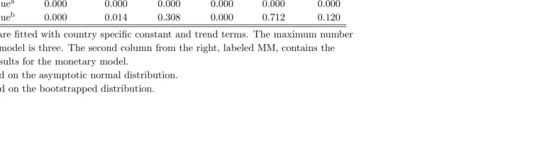
Table 1 shows the panel stationary test results for each variable. For each model, the first row contains the test value, the second row contains the asymptotic p-value, and the third row contains the bootstrappedp-value. The test results for the no break model suggest
5
that the null hypothesis of stationary can be safely rejected, since the asymptotic p-value is zero for all variables. However, these p-values are computed under the assumption of cross-section independence, which is unlikely to hold in this particular context. Therefore, in order to account for this dependence, we use the bootstrappedp-values. As can be seen, the conclusions are not altered by taking the cross-sectional correlation into account, at least not at the 10 percent level.
Turning now to the model with breaks, we see that both the asymptotic and bootstrapped p-values indicate that the presence of structural breaks does not interfere with the results obtained from the no break model. One exception is relative output, for which we are unable to reject the null of stationarity at the 10 percent level. However, if we omit the trend and only allow for a breaking intercept, then the null is again strongly rejected. Therefore, since the overall evidence in favor of a rejection is quite overwhelming, we choose to proceed as if all the variables are in fact nonstationary.
4.3 Cointegration tests
The second step in our analysis is to test whether the variables are cointegrated, as predicted by the monetary model. The bulk of the existing evidence based on panel data indicate that cointegration, and thus also the monetary model, holds. However, as pointed out in the introduction, most existing studies are generally quite restrictive in nature, which greatly increases the risk of misleading conclusions.
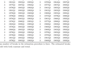
The leftmost panel of Table 2 reports the estimated breakpoints obtained as a bi-product when applying the Z(M) test to the model with breaks. With the exception of Australia, we see that three breaks are found for all countries. Thus, for all countries but Australia, we end up estimating the maximum number of breaks. This is in agreement with the results of Perron (1997), who point out that the type of information criteria used here cannot take into account the effect of different distributions of the data and possible serial correlation in the regression errors. In fact, as Perron (1997) showed in simulations, although most criteria perform reasonably well when the errors are not correlated, they have a strong tendency to overestimate the number of breaks when serial correlation is present. Of course, the purpose in this paper is not the correct estimation of the number of breaks per se but rather the accounting of the effects of these breaks. Thus, overestimation is not a serious problem in the sense that the model is still free to estimate the associated break parameters to zero.
Looking at Table 2 we see that there is a preponderance of breaks located around the middle of the sample, which seem very reasonable from an historical point of view with events such as oil price shocks, the formation of European Monetary System and, in particular, the rise and fall of the dollar. Specifically, while the breaks found in the late 1970’s agree with the oil price shocks of that period, the breaks in the early 1980’s are more likely to reflect the start of appreciation of the dollar, with the breaks in the middle of the 1980’s reflecting the subsequent transition from dollar appreciation to dollar depreciation. The breaks in the early 1990’s can be attributed to the formation of European Monetary System when most European countries abolished their capital controls. Another possibility is that these breaks reflect the end of the dollar depreciation in 1987.
Thus, we see that the break date estimator is able to correctly identify most of the major structural events in the sample. Interestingly, these are exactly the events thought to have shifted the PPP relation during this period, see Papell (2002) for a more thorough discussion. This is important because it suggests that the observed breaks in the monetary model may well be due to breaks in the underlying PPP relation. We will elaborate on this in the next section.
4.4 The PPP relationship
period. A natural way to test this hypothesis is to estimate and test the PPP relationship for structural breaks. If our story is correct, the estimated breakpoints should match those presented for the monetary model in Table 2. In order to perform this test, we follow the recommendation of Papell (2002) and Papell and Prodan (2006), and estimate the following model with breaks in both the intercept and trend
sit = µij+τijt+δi(pit−p∗t) +eit, (9)
whereδi is a country specific slope. As before, the indexj indicates the breaks. If the trend
qualified version of PPP holds, then the disturbance eit should be stationary so that the
[image:14.595.103.496.359.631.2]nominal exchange rate and the relative price level are cointegrated. To test whether this is in fact the case, we again employ theZ(M) test.
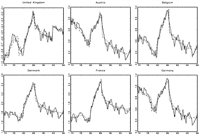
Figure 1: Nominal dollar exchange rates with fitted trend functions.
Similar to the results of the monetary model, the results reported in Table 1 suggest that the PPP relation emerges only once the presence of cross-country dependence and structural breaks has been taken into account.6
These results are consistent with Papell (2002) and
6
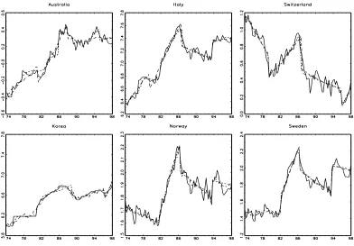
Figure 2: Nominal dollar exchange rates with fitted trend functions.
[image:15.595.104.496.453.726.2]Papell and Prodan (2006), who also find that PPP must be rejected unless the possibility of structural breaks is entertained.
In view of this, we now proceed to examine the estimated PPP breaks reported in the rightmost panel of Table 2. It is seen that, within a few quarters accuracy, almost all of the breaks in the monetary model can be derived from breaks in the underlying PPP relationship. Hence, it appears as that the instability of the monetary model can be largely explained by an instable PPP relation.
To further illustrate the connection between the monetary model and PPP relation, Fig-ures 1 to 3 plot the nominal exchange rates together with the fitted trend functions for the model with breaks in both constant and trend. The solid line represents the nominal ex-change rate, the semisolid line represents the monetary model, and the dashed line represents the PPP relation. It can easily be seen that nearly all exchange rates exhibit several breaks in the 1980’s, most of which seem to reflect the appreciation and depreciation of the dollar. More importantly, we see that the trend lines for both the monetary and PPP models seem to provide a very good fit to the nominal exchange rate for all 18 countries. The fact that the two trend lines appear to follow each other so closely gives an indication as to the importance of the PPP relation in the monetary model.
5
Conclusions
This paper reconsiders the possibility of cointegration between the nominal exchange rate and its fundamentals, as specified by the monetary exchange rate model. The methodological approach used for this purpose is flexible enough to accommodate a large degree of country specific heterogeneity, cross-country dependence as well as multiple structural breaks.
Based on data for 18 industrialized countries between 1973Q1 and 1997Q1, we find that the evidence in favor of the monetary model depends upon whether cross-country dependence and structural breaks are considered or not. When the effects of cross-country dependence and breaks are ignored, the monetary model fails, whereas when these effects are taken into account, the monetary model seems to hold. Consistent with other studies, we find that three breaks are sufficient to capture the episodic behavior of the dollar exchange rates in the 1980’s, and that the locations of the estimated breaks correspond well with the structural shifts in the underlying PPP relationship.
can be improved by allowing for breaks in the forecasting regression. Thus, the poor forecast-ing performance noted by Meese and Rogoff (1983) and the subsequent literature on exchange rate predictability may simply be due to the fact that the parameters in the estimated model have not been stable.7
As we have demonstrated, one possible explanation for this instability is that the underlying PPP relation may have been unstable too.
7
References
Bai, J., and Perron, P. (1998). Estimating and testing linear models with multiple structural changes. Econometrica 66, 47–78.
Bai, J., and Perron, P. (2003). Computation and analysis of multiple structural change models. Journal of Applied Econometrics 18, 1–22.
Basher, S.A. and Carrion-i-Silvestre, J. L. (2008). Price level convergence, purchasing power parity and multiple structural breaks in panel data analysis: An application to US cities. Forthcoming in Journal of Time Series Econometrics.
Breitung, J., and Pesaran, M. H. (2008). Unit roots and cointegration in panels. In Matyas, L., and Sevestre, P. (Eds.), The Econometrics of Panel Data. Third edition, Ch. 9, 279–322. Kl¨uwer Academic Publishers.
Carrion-i-Silvestre, J. L., Del Barrio-Castro, T., and L´opez-Bazo, E. (2005). Breaking the panels: An application to the GDP per capita. Econometrics Journal 8, 159–175.
Goldberg, M.D. and Frydman, R. (1996). Empirical exchange rate models and shifts in the co-integrating vector. Journal of Structural Change and Economic Dynamics7, 55–78.
Groen, J. J. J. (2000). The monetary exchange rate model as a long-run phenomenon.
Journal of International Economics 52, 299–319.
Groen, J. J. J. (2002). Cointegration and the monetary exchange rate model revisited.
Oxford Bulletin of Economics and Statistics 64, 361–380.
Harris, D., Leybourne, S., and McCabe, B. (2005). Panel stationarity tests for purchas-ing power parity with cross-sectional dependence. Journal of Business and Economic Statistics 23, 395–409.
Hegwood, N. D., and Papell, D. H. (1998). Quasi purchasing power parity. International
Journal of Finance and Economics 3, 279–289.
Im, K.-S., Lee, J., and Tieslau, M. (2005). Panel LM unit-root tests with level shifts. Oxford
Bulletin of Economics and Statistics 67, 393–419.
Mark, N. C., and Sul, D. (2001). Nominal exchange rates and monetary fundamentals: Evidence from a small post-Bretton Woods panel. Journal of International Economics 53, 29–52.
Meese, R. A., and Rogoff, K. (1983). Empirical exchange rate models of the seventies: Do they fit out of sample? Journal of International Economics 14, 3–24.
Newey, W., and West, K. (1994). Autocovariance lag selection in covariance matrix estima-tion. Review of Economic Studies 61, 631–653.
O’Connell, P. G. J. (1998). The overvaluation of purchasing power parity. Journal of
Papell, D. (2002). The great appreciation, the great depreciation, and the purchasing power parity hypothesis. Journal of International Economics 57, 51–82.
Papell, D., and Prodan, R. (2006). Additional evidence of long run purchasing power parity with restricted structural change. Journal of Money, Credit and Banking 38, 1329– 1349.
Perron, P. (1997). L’estimation de mod`eles avec changements structurels multiples. Actualit
conomique 73, 457–505.
Phillips, P. C. B., and Hansen, B. E. (1990). Statistical inference in instrumental variables regression withI(1) process. Review of Economics Studies 57, 99–125.
Rapach, D. E., and Wohar, M. E. (2002). Testing the monetary model of exchange rate de-termination: New evidence from a century of data. Journal of International Economics 58, 359–385.
Rapach, D. E., and Wohar, M. E. (2004). Testing the monetary model of exchange rate determination: A closer look at panels. Journal of International Money and Finance 23, 867–895.
Sarantis, N. (1994). The monetary exchange rate model in the long run: An empirical investigation. Weltwirtschaftliches Archive 130, 698–711.
Taylor, A. M., and Taylor, M. P. (2004). The purchasing power parity debate. Journal of
Economic Perspectives 18, 135–158.
Westerlund, J. (2005). Testing for panel cointegration with multiple structural breaks. Ox-ford Bulletin of Economics and Statistics 68, 101–132.
Table 1: Panel stationarity and cointegration tests.
Stationarity tests Cointegration tests Model Test sit (mit−m∗t) (yit−yt∗) (pit−p∗t) MM PPP
No breaks Value 17.310 22.403 12.308 27.456 16.641 16.125
p-valuea
0.000 0.000 0.000 0.000 0.000 0.000
p-valueb
0.090 0.012 0.098 0.000 0.002 0.008
Breaks Value 10.781 9.582 4.346 11.625 12.288 10.478
p-valuea
0.000 0.000 0.000 0.000 0.000 0.000
p-valueb
0.000 0.014 0.308 0.000 0.712 0.120
Notes: The models are fitted with country specific constant and trend terms. The maximum number breaks in the break model is three. The second column from the right, labeled MM, contains the cointegration test results for the monetary model.
a
Thep-value is based on the asymptotic normal distribution. b
Thep-value is based on the bootstrapped distribution.
Table 2: Estimated breaks.
Monetary model PPP
Country No. Break 1 Break 2 Break 3 No. Break 1 Break 2 Break 3
Australia 2 1980Q2 1987Q1 − 3 1985Q1 1990Q2 1994Q2
Austria 3 1981Q1 1984Q4 1987Q2 3 1980Q4 1985Q4 1995Q1 Belgium 3 1980Q4 1985Q4 1995Q1 3 1981Q1 1985Q4 1995Q1 Denmark 3 1981Q1 1985Q4 1995Q1 3 1978Q4 1984Q4 1987Q2 Canada 3 1977Q1 1987Q1 1992Q1 3 1977Q1 1987Q1 1992Q1 Finland 3 1979Q3 1985Q3 1992Q4 3 1981Q1 1985Q4 1992Q3 France 3 1981Q1 1985Q3 1992Q4 3 1981Q1 1985Q3 1988Q2 Germany 3 1978Q3 1985Q3 1988Q2 3 1980Q4 1985Q4 1995Q1 Greece 3 1979Q3 1986Q1 1992Q4 3 1975Q3 1979Q4 1986Q2 Italy 3 1978Q3 1985Q4 1992Q4 3 1981Q1 1986Q1 1992Q4 Japan 3 1978Q1 1986Q1 1995Q1 3 1977Q4 1986Q1 1995Q1 Korea 3 1982Q3 1989Q1 1995Q2 3 1980Q1 1988Q1 1995Q3 Netherland 3 1978Q4 1985Q3 1988Q2 3 1980Q4 1985Q4 1995Q1 Norway 3 1980Q4 1985Q3 1992Q4 3 1980Q4 1985Q3 1992Q4 Spain 3 1979Q1 1983Q3 1992Q4 3 1979Q1 1985Q3 1992Q4 Switzerland 3 1978Q3 1986Q1 1995Q1 3 1978Q3 1985Q4 1995Q1 Sweden 3 1981Q2 1985Q3 1992Q4 3 1981Q2 1985Q3 1992Q4 United Kingdom 3 1979Q1 1985Q3 1992Q4 3 1980Q2 1985Q2 1992Q4
Notes: The maximum number of breaks in the estimation procedure is three. The estimated breaks are based on the model with both constant and trend.