http://dx.doi.org/10.4236/ojms.2014.41004
Modeling Ocean Chlorophyll Distributions by
Penalizing the Blending Technique
Mathias A. Onabid1, Simon Wood2 1
Department of Maths-Computer Science, Faculty of Sciences, University of Dschang, Dschang, Cameroon 2
Department of Mathematical Sciences, University of Bath, Bath, UK Email: mathakong@yahoo.fr, s.wood@bath.ac.uk
Received September 6, 2013; revised October 19, 2013; accepted November 12, 2013
Copyright © 2014 Mathias A. Onabid, Simon Wood. This is an open access article distributed under the Creative Commons Attribu- tion License, which permits unrestricted use, distribution, and reproduction in any medium, provided the original work is properly cited. In accordance of the Creative Commons Attribution License all Copyrights © 2014 are reserved for SCIRP and the owner of the intellectual property Mathias A. Onabid, Simon Wood. All Copyright © 2014 are guarded by law and by SCIRP as a guar- dian.
ABSTRACT
Disparities between the in situ and satellite values at the positions where in situ values are obtained have been the main handicap to the smooth modeling of the distribution of ocean chlorophyll. The blending technique and the thin plate regression spline have so far been the main methods used in an attempt to calibrate ocean chlorophyll at positions where the in situ field could not provide value. In this paper, a combination of the two techniques has been used in order to provide improved and reliable estimates from the satellite field. The thin plate regression spline is applied to the blending technique by imposing a penalty on the differences between the satellite and in
situ fields at positions where they both have observations. The objective of maximizing the use of the satellite
field for prediction was outstanding in a validation study where the penalized blending method showed a re- markable improvement in its estimation potentials. It is hoped that most analysis on primary productivity and management in the ocean environment will be greatly affected by this result, since chlorophyll is one of the most important components in the formation of the ocean life cycle.
KEYWORDS
In Situ, Satellite; Ship and Buoy; Penalized Regression Spline; Penalty; Penalized Blending
1. Introduction
A detailed study of the ocean environment and its con- stituent elements are of utmost importance in guiding decision-makers on policies regarding marine activities such as fishing and their consequences for human life and society as a whole. In the ocean food chain, phytop- lankton, which are found in the upper layer of the ocean, are of extreme importance. Indeed, aquatic life and pro- duction revolve about the distribution and biomass of these unicellular algae. Thus, to better understand the ocean food chain, it is necessary to track their existence and monitor their population distribution in the ocean environment. To measure their population by cell counts is very difficult, because of their resemblance to other non-algae carbon rich particles. An alternative method of doing this is in terms of their photosynthetic pigment
content, chlorophyll, which is endemic across all tax-
data obtained by ship and buoy (in situ) and the noisiness of the satellite field [7]. These factors have been the main handicap to the smooth calibration of ocean chlorophyll estimates from the satellite observations. The penalized re- gression splines are a technique that could be used to model noisy data [8]. The use of this statistical technique in the calibration of ocean chlorophyll was also suggested by [1].
The objective of this article, therefore, is to demon- strate how the principles of penalized regression could be applied to the blending process in order to obtain better estimate of ocean chlorophyll from the satellite data field. The approach would mainly address the noisiness of the data fields by introducing a penalty on the differences between their observations at positions where both fields have values. The belief is that, by penalizing the differ- ences between the satellite and the in situ fields, the sa- tellite will become closer to the in situ field and can thus be used to sufficiently estimate ocean chlorophyll values at positions where the in situ field could not provide val- ues. Since the process of penalization involves smooth- ing, the efficiency of the technique will depend on the choices of the smoothing parameters.
Inspiration to this was drawn from the interpolation equation
(
)
(
)
(
)
blend , sat , 1 ,
n k k
f x y = f x y
∑
= g x y (1)found in Onabid (2011) in the section dealing with the proof as to why results from the corrector factor and the smooth in-fill methods should coincide. From this equa- tion, the term of interest is
(
)
1
,
n k k
g x y
=
∑
which is the sum of the solution to the partial differential
equation obtained at each boundary point k where there is
a difference between the satellite and in situ value. In
order to penalize these differences, the interpolation Eq- uation (1) had to be represented using basis functions. Consider the equation
( )
( )
( )
blend sat
1
, , , ,
n k k
f x y f x y g x y
=
=
∑
where g k is actually the solution to
2 2
2 2 0,
g g x y
∂ ∂
+ =
∂ ∂ (3)
subject to the boundary conditions
{
0; ;x y ii i: =1;;k−1;k+1;; ;n∆k;x yk; k}
. This Equation (2) can be re-written with each of thek
g separately as
( )
( )
( )
blend sat
1
, , , ,
n k k k
f x y f x y β x y
=
=
∑
∆ (4)where βk is set to the difference between the in situ and
satellite values at boundary point k and Δk(x; y) repre-
senting the basis function is the solution to
2 2
2 2 0
g g x y
∂ ∂
+ =
∂ ∂ (5)
with external boundary points set to zero and the internal
boundary points set to zero everywhere except at the kth
position where it is set to 1.0, that is the knot of the basis. What this means is that, for each internal boundary
point (knot), the blending process is performed to esti-
mate the entire blended field with that particular boun- dary point acting as the only boundary point for the pro- cess. During the process, the value of this boundary point equals 1.0 and the resulting field is the basis for this knot.
The blended field corresponding to this particular knot is
obtained by multiplying the original knot value with its
basis. Blended fields obtained from each of the knots are summed up. This sum is then added to the satellite field
to obtain the final blended field which we call the basis
blend.
2. Penalizing the Blending Process
For the penalized regression spline to be applied, it was necessary to represent the term of interest in the blending process as a regression equation.
Representing Blending as a Regression Equation
Considering the Equation (4) which is the interpolation form of the blending process represented using basis functions, also consider the fact that the objective is to
control the differences between the satellite and the in
situ fields, it is obvious that focus here should be on the
term
( )
1
, ,
n k k k
x y
β
=
∆
∑
from where the βkss′ could be estimated by penalized
least squares in order to minimize the effect of these dif- ferences and consequently maximize the use of the sate- llite field as estimate to ocean chlorophyll at points
where in situ could not provide observations
Let
(
)
(
)
log insitu log satellite ;
k k k
Z = −
be calculated for each point it K, where satellite and in
situ have observations. This can be written as a regres-
sion equation of the form,
(
)
1
,
n
k j j j j k
j
Z β x y ε
=
=
∑
∆ + (6)and εk the error term. This expression is equal to
(
,)
k k k k k k
Z =β ∆ x y +ε
Thus if Zkis expressed using the basis space, one ob-
tains this model;
(
)
(
)
(
)
(
)
1 1 1 1 2 2 2 2 3 3 3 3
k
n n n n k
Z x y x y x y
x y
β β β
β ε
= ∆ + ∆ + ∆
+ + ∆ +
Fitting this model by least squares will simply result in the interpolation scheme since there is exactly one para- meter per datum, thus nonparametric techniques were then explored. The thin plate regression spline was then used to introduce a penalty to this blending regression equation.
3. Penalizing the Blending Regression
Equation
From Equation (6), the control of the smoothness of the differences can be achieved by either altering the basis dimension, that is changing the number of selected knots or keeping the basis dimension fixed and then adding a
penalty term to the least squares objective. The later was used. Therefore the penalized least squares objective will be to minimize
(
)
2(
(
)
)
1
, ,
n
k k k k k k k k k
k
Z β x y λ β x y
=
− ∆ + ∆
∑
J (7)where J is a penalty function which penalizes model
wiggliness while model smoothness is controlled by the
smoothing parameter λ, as described by [9]. As a first
step in estimating the penalized least squares objective, the simple penalized least squares technique of ridge regression was used. In this process, the intention is to penalize each of the parameters separately by introducing a penalty to each of the estimated parameters. Following this method, the penalized least squares objective will be to minimize
( )
(
)
2 21 , 1
n n
p k k k k k k k k k
Q β =
∑
= Z − ∆β x y +λ∑
= β (8)with respect to βks′: The penalty is represented by the
term λk
∑
nk=1βk2 with λ being the smoothing para- meter to control the trade off between model fit and model smoothness. Thus the problem of estimating the degree of smoothness of the model is now the problem ofestimating the smoothing parameter λ.
Assuming that the smoothing parameter is given, how
then can the βks′ be estimated in this penalized least
squares objective?
From Equation (8), the term Δk(xk; yk) reduces to a n×n
identity matrix. Now, define an augmented Z, say Z; as
[
]
T1 n 0 0
Z Z
=
Z (with n zeroes) which can
also be augmented directly in the objective.
When this is done, Equation (8) could now be written as
( )
2 0 n p n I Z Q I β β λ = − From here, ˆβ can be calculated as follows:
(
)
1 1 ˆ 0 1 nn n n n
n n
I Z
I I I I
I
I Z
β λ λ
λ λ − − = = +
with ˆ 1
1
Z β
λ
=
+ ; this implies that,
2 2 2 2 2 1 ˆ 1 1 1
Z I Z Z Z
Z λ β λ λ λ λ = − = − = + + +
3.1. Choosing How Much to Smooth
This refers to the selection of the smoothing parameter
λ. This must be done with care such that the selected
value should be suitable, so much so that if the true
smooth function is f the estimated smooth function ˆf ,
should be as close as possible to it. The reason being if
λ is too high, the data will be over-smoothed and if it is
too low, the data will be under-smoothed hence the re- sulting estimate will not be close to the true function. The
aim as described by [9] will be to select a λ which will
minimize the difference between ˆf and f that is to say
if M is the difference, then λ should minimize
(
)
2 01 n ˆ
i i i f f n = =
∑
− MThis could have been easier if the true values for f ex-
isted already. Because this is not the case, the problem
was approached by deriving estimates of M plus some
variation. This was achieved by making use of the ordi- nary cross validation (OCV) technique. In this technique, a model is fitted to the rest of the data, when a datum is left out. The squared difference between the datum and its predicted value from the fitted model is calculated. This is done for all the points and the mean taken over all the data. Thus the ordinary cross validation criterion is written as
[ ]
(
)
2 00 1 n ˆ
i i i i f Z n − = =
∑
− Vwhere fˆi[ ]i −
is the estimate from the model fitted to all data except Zi. The idea of calculating V0 each time leav-
(
)
20 2
0
ˆ 1
(1 )
n i i
i ii
f Z n = A
− =
−
∑
V
where ˆf is the estimate from fitting to all the data and
A is the corresponding influence matrix.
[9] Emphasizes the fact that though OCV is a reasona- ble way of estimating smoothing parameters, it has the drawbacks of being computationally expensive to mi- nimize in the case of additive models where there could be many smoothing parameters and secondly it has a slightly disturbing lack of invariance. Thus in practice,
the weights 1−Aiiare often replaced by the mean weight
tr(I − A)/n in order to arrive at the generalized cross validation (gcv) score given as
(
)
(
)
2 0
g 2
ˆ
I A
n
i i
i
n Z f
tr
= −
=
−
∑
V
This has the computational advantage over OCV and can also be argued to have some advantages in terms of invariance. Therefore, an easy way to look for the best smoothing parameter would be to search through a se-
quence of λ′s, each time fitting a penalized regression
model with the new λ value and calculating the gcv
score. At the end, the λ value corresponding to the
lowest gcv score will be the optimal smoothing parame- ter.
3.2. Calculating the gcv Score
Amongst the techniques of ridge regression, integrated least squares, integrated squared derivatives and efficient method used in computing the gcv score, only the effi- cient method herein described provided and better esti- mate for the gcv score.
Efficient Calculation of the gcv Score
The idea here is to provide a means of obtaining opti- mum values for the gcv score, the degree of freedom tr(A)
and the smoothing parameter λ which will minimize
the gcv score. These will be very important since the objective is to build a model that will produce estimates in the blended field which are as close as possible to the true field. The QR decomposition described in [10] will be used because it is believed that QR is more stable than the Cholesky decomposition. This was achieved as fol- lows.
The objective is to minimize
2 T
y−Xβ +λβ βS
with respect to β .
ˆ
Xβ Ay
⇒ =
where
(
T)
1 T.
A=X X X+λS − X
The corresponding gcv score for the given λ is then
given as
( )
( )
2 2
n y Ay V
n tr A
λ = −
−
In order to calculate the efficient gcv score, let X = QR
where R is the upper triangle and Q consist of the col-
umns of an orthogonal matrix such that QTQ = I but
T
QQ ≠I
(
T)
1 T T(
T 1)
1 TA QR R R λS − R Q Q I λR SR− − − Q
⇒ = + = +
From an eigen-decomposition
T 1 T
R SR− − =UDU
where D is a diagonal matrix of eigen values, the col-
umns of U are eigenvectors and U is orthogonal.
(
)
( )
1 T T
1 1
i ii
A QU I D U Q tr A
D
λ
λ
−
⇒ = +
⇒ =
+
∑
(9)(
)
(
)
2 T T T
1 2
T T T
2
ˆ ˆ ˆ ˆ
2
y Ay y y y Ay y AAy
y y y I λD − y y I λD − y
− = − +
= − + + + (10)
where yˆ=U Q yT T .
From Equations (9) and (10) it follows that V
( )
λcould be evaluated very cheaply for each new λ since
the QR and eigen-decompositions are only needed once.
The smoothing parameter
( )
λ corresponding to eachof these lowest gcv scores were then use in fitting the penalized regression models. The results obtained are then compared to those from the other techniques.
4. Validating the Blended Fields Obtained
from the Various Blending Methods
The strength of this method in predicting existing in situ
observation was compared to that of the normal blending method. Because penalizing the blending method had to make use of the basis function, the blended field obtained from the basis function method was also compared. Since the basis function method works by the use of a basis set (knots), after the selection of the validation data set the
remaining in situ observations were then used as knots
for the basis function blending method. The penalized blended field was obtained by using parameters obtained from the efficient method of calculating gcv as described in Section 3.2.1. Randomly selected validation data sets
each containing 175 observations from the observed in
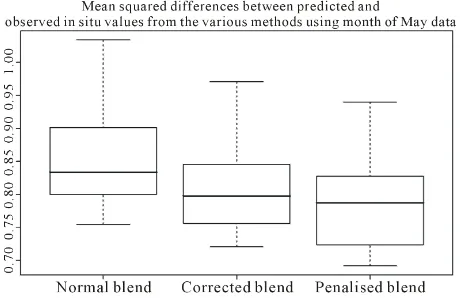
ber of observations in the in situ field. The mean squared
differences between the predicted and the observed in
situ values were computed and plotted (Figure 1). There was not so much difference between predictions from the basis and the penalized. Though most of the times the differences are visible only after the third or fourth decimal place, there are a few times where the dif- ferences appear very distinct between the two in favour of the penalized blending method. Penalized models are always expected to perform better than non penalized ones. The poor performance here could have been caused by the choice of the smoothing parameter which is being obtained in this case by cross validation.
5. Discussions
We have been able to successfully establish a procedure for implementing smoothing on the blending process by making use of corrector factor blending technique model of [7]. This was achieved by expressing the interpolation formula used by the corrector factor blending technique in a form making use of the basis function. The aim of expressing the blending process using basis functions was to pave the way to implement penalization. This was implemented by adding a penalty term to the least squares objective. This term contained the penalty func- tion which penalizes the model and a smoothing parame- ter to control the smoothness of the model. The main issue here was to be able to choose the right smoothing parameter such that the estimated smooth function should be as close as possible to the true function. Cross valida- tion technique was used to obtain the smoothing parame- ter. To obtain the cross validation score three techniques were used, namely ridge regression, integrated least squares and the integrated squared derivative.
[image:5.595.58.288.552.701.2]Calculating the cross validation score using ridge re- gression failed because the final expression for calculat- ing the score did not depend on the smoothing parameter.
Figure 1. A box plot of the mean squared differences be-
tween predicted and observed in situ values from the dif- ferent blending methods.
As described by [9], this is not surprising since if a Zkis
dropped from the model sum of squares term in equation
(8), the only thing influencing the estimate of βk would
be the penalty term, which will be minimized by setting 0
k
β = ,whatever positive value the smoothing parame-
ter takes. This complete decoupling will cause cross- validation to fail. Thus, if a datum is left out, its corres- ponding estimate will always be zero since no other data has influence on it. This behavior occurs for any possible value of the smoothing parameter.
Making use of the cross-validation score calculated from the integrated least squares did not improve on the results in this research. This again, according to [9], is not surprising because if one considers any three equally spaced points x1, x2, x3 with corresponding f(xi) values to
be µ1, µ2 and µ3. Also, if µ1 µ3 µ
∗
= = then in or-
der to minimize
( )
3 12 d
x
x µ x x
∫
one should set µ2 µ 2
∗
= . This condition does not hold
for the data fields used in this research since the data fields were sparse, and the missing values were replaced by pseudo zeroes, so it was not uncommon to find a set of three adjacent points with similar values. In a situation like this, [9] states that, if the middle point is omitted from the fitting, the action of the penalty will send its estimate to the other side of zero from its neighbors. Meaning that a better prediction of the omitted datum will only be possible with a high smoothing parameter and this will be closer to zero since the high smoothing parameter will tend to shrink the values of the other in- cluded points towards zero and hence the omitted point. With this, cross validation will also have the tendency to always select an estimate for the omitted points closer to zero from the model. This could have been the cause of the poor results obtained. The integrated squared deriva- tive penalty is not expected to suffer from the same problems faced by the previous methods. This is because the action of the penalty is simply to try and flatten the smooth function around the vicinity of the omitted datum. If the smoothing parameter is large, it will increase the flattening and consequently pulls the estimate far away from the omitted datum. The penalty obtained by this technique had very little or no effect on the smoothing function hence the equality in results from the penalized and the basis function model.
6. Conclusion
blending method. The penalized model was obtained by first representing the blending method by making use of the basis function which was also considered as a model on its own. Even though the results from the basis func- tion and penalized model were relatively identical since most differences occurred at the third or fourth decimal place, it is important to know that the difference between these methods and the normal blending method is quite
alarming (Figure 1) and therefore should be encouraged
especially if more data could be obtained from ship and buoy. With the emergence of this result, it is hoped that most of the analysis on primary productivity and man- agement in the ocean environment will be greatly af- fected, since chlorophyll is one of the most important components in the formation of the ocean life cycle.
Future Work
The failure of the penalized blending regression models to perform better than the basis function model could have been because the right penalty was not obtained. Therefore, more work could be done towards obtaining other penalties. Maybe, an integrated squared second derivative could be tried or one could try a combination of the first and second derivatives (double penalization). To enable the blending process to be very close to reality, the possibility of extending it to three dimensions could be looked into.
REFERENCES
[1] E. Clarke, D. Speirs, M. Heath, S. Wood, W. Gurney and S. Holmes, “Calibrating Remotely Sensed Chlorophyll-a Data by Using Penalized Regression Splines,” Journal of Royal Statistics Society,Series C, Vol. 55, No. 3, 2006,
pp. 331-353.
[2] R. W. Eppley, E. Stewart, M. R. Abbott and U. Heyman, “Estimating Ocean Primary Production from Satellite Chlorophyll. Introduction to Regional Differences and Statistics for the Southern California Bight,” Journal of Plankton Research, Vol. 7, No. 1, 1985, pp. 57-70. http://dx.doi.org/10.1093/plankt/7.1.57
[3] D. A. Flemer, “Chlorophyll Analysis as a Method of Eva- luating the Standing Crop Phytoplankton and Primary Productivity,” Chesapeake Science, Vol. 10, No. 3-4, 1969, pp. 301-306.http://dx.doi.org/10.2307/1350474
[4] A. H. Oort, “Global Atmospheric Circulation Statistics,” NOAA Prof Paper 14 180pp Nat. Oceanic and Atmos- pheric Administration Silver Spring, Maryland, 1983. [5] R. W. Reynolds, “A Real-Time Global Sea Surface Tem-
perature Analysis,” Journal of Climate, Vol. 1, No. 1, 1988, pp. 75-87.
http://dx.doi.org/10.1175/1520-0442(1988)001<0075:AR TGSS>2.0.CO;2
[6] W. W. Gregg and M. E. Conkright, “Global Seasonal Climatologies of Ocean Chlorophyll: Blending in Situ and Satellite Data for Coastal Zone Colour Scanner Era,” Journal of Geophysical Research, Vol. 106,No. C2, 2001, pp. 2499-2515.http://dx.doi.org/10.1029/1999JC000028 [7] M. A. Onabid, “Improved Ocean Chlorophyll Estimate
from Remote Sensed Data: The Modified Blending Tech- nique,” African Journal of Environmental Science and Technology, Vol. 5, No. 9, 2001, pp. 732-747.
[8] S. N. Wood, “Thin Plate Regression Splines,” Royal Sta- tistical Society, Series B, Vol. 65, No. 1, 2003, pp. 95-114. http://dx.doi.org/10.1111/1467-9868.00374
[9] S. N. Wood, “Generalized Additive Models: An Introduc- tion with R,” Chapman and Hall/CRC, London, 2006. [10] R. Scraton, “Further Numerical Methods in Basic,” Ed-