Time phase bispectral analysis

Time-phase bispectral analysis

Janez Jamsˇek,1,2,3,*Aneta Stefanovska,1,3,†Peter V. E. McClintock,3,‡and Igor A. Khovanov3,4,§ 1

Group of Nonlinear Dynamics and Synergetics, Faculty of Electrical Engineering, University of Ljubljana, Trzˇasˇka 25, 1000 Ljubljana, Slovenia

2_{Department of Physics and Technical Studies, Faculty of Education, University of Ljubljana, Kardeljeva plosˇcˇad 16,} 1000 Ljubljana, Slovenia

3_{Department of Physics, University of Lancaster, Lancaster LA1 4YB, United Kingdom} 4_{Laboratory of Nonlinear Dynamics, Saratov State Unversity, 410026 Saratov, Russia}

共Received 8 January 2003; published 3 July 2003兲

Bispectral analysis, a technique based on high-order statistics, is extended to encompass time dependence for the case of coupled nonlinear oscillators. It is applicable to univariate as well as to multivariate data obtained, respectively, from one or more of the oscillators. It is demonstrated for a generic model of interacting systems whose basic units are the Poincare´ oscillators. Their frequency and phase relationships are explored for different coupling strengths, both with and without Gaussian noise. The distinctions between additive linear or quadratic, and parametric共frequency modulated兲, interactions in the presence of noise are illustrated.

DOI: 10.1103/PhysRevE.68.016201 PACS number共s兲: 05.45.Df, 02.70.Hm, 05.45.Xt

I. INTRODUCTION

Most real systems are nonlinear and complex. In general, they may be regarded as a set of interacting subsystems; given their nonlinearity, the interactions can be expected to be nonlinear too.

The phase relationships between a pair of interacting os-cillators can be obtained from bivariate data 共i.e., where the coordinate of each oscillator can be measured separately兲by use of the methods recently developed for analysis of syn-chronization, or generalized synsyn-chronization, between cha-otic and/or noisy systems. Not only can the interactions be detected关1兴, but their strength and direction can also be de-termined 关2兴. The next logical step in studying the interac-tions among coupled oscillators must be to determine the nature of the couplings: the methods developed for synchro-nization analysis are not capable of answering this question. Studies of higher-order spectra, or polyspectra, offer a promising way forward. The approach is applicable to inter-acting systems quite generally, regardless of whether or not they are mutually synchronized. Following the pioneering work of Brillinger and Rosenblatt 关3兴, increasing applica-tions of polyspectra in a diversity of fields have appeared, e.g., telecommunications, radar, sonar, speech, biomedical, geophysics, imaging systems, surface gravity waves, acous-tics, econometrics, seismology, nondestructive testing, oceanography, plasma physics, and seismology. An extensive overview can be found in Ref.关4兴. The use of the bispectrum as a means of investigating the presence of second-order nonlinearity in interacting harmonic oscillators has been of particular interest during the last few years 关5– 8兴.

Systems are usually taken to be stationary. For real sys-tems, however, the mutual interaction among subsystems

of-ten results in time variability of their characteristic frequen-cies. Frequency and phase couplings can occur temporally, and the strength of coupling between pairs of individual os-cillators may change with time. In studying such systems, bispectral analysis for stationary signals, based on time av-erages, is no longer sufficient. Rather, the time evolution of the bispectral estimates is needed.

Priestley and Gabr关9兴were probably the first to introduce the time-dependent bispectrum for harmonic oscillators. Most of the subsequent work has been related to the time-frequency representation and is based on high-order cumu-lants 关10兴. The parametric approach has been used to obtain approximate expressions for the evolutionary bispectrum

关11兴. Further, Perry and Amin have proposed a recursion method for estimating the time-dependent bispectrum 关12兴. Dandawate´ and Giannakis have defined estimators for cyclic and time-varying moments and cumulants of cyclostationary signals 关13兴. Schack et al. 关14兴 have recently introduced a time-varying spectral method for estimating the bispectrum and bicoherence: the estimates are obtained by filtering in the frequency domain and then obtaining a complex time-frequency signal by inverse Fourier transform. They assume, however, that the interacting oscillators are harmonic.

Millingen et al. 关15兴introduced the wavelet bicoherence and were the first to demonstrate the use of bispectra for studying interactions among nonlinear oscillators. They used the method to detect periodic and chaotic interactions be-tween two coupled van der Pol oscillators, but without con-centrating on time-phase relationships, in particular.

In this paper we develop an approach关16兴that introduces time dependance to the bispectral analysis of univariate data. We focus on the time-phase relationships between two 共or more兲 interacting systems. As we demonstrate below, the method enables us to detect that two or more subsystems are interacting with each other, to quantify the strength of the interaction, and to determine its nature, whether additive lin-ear or quadratic, or parametric in one of the frequencies. It yields results that are applicable quite generally to any sys-tem of coupled nonlinear oscillators. Our principal motiva-*Electronic address: [email protected]

†_{Electronic address: [email protected]}

‡_{Electronic address: [email protected]}

§_{Electronic address: [email protected]}

press Gaussian noise of unknown spectral form, and to detect and characterize signal nonlinearities关5兴. In what follows we extend bispectral analysis to extract useful features from nonstationary data, and we demonstrate the modified tech-nique by application to test signals generated from coupled oscillators.

The bispectrum involves third-order statistics. Spectral es-timation is based on the conventional Fourier type direct approach, through computation of the third-order moments which, in the case of third-order statistics, are equivalent to third-order cumulants 关5,18 –21兴.

The classical bispectrum estimate is obtained as an aver-age of estimated third-order moments 共cumulants兲Mˆ₃i(k,l),

Bˆ共k,l兲⫽1 K

兺

K

Mˆ₃i共k,l兲, 共1兲

where the third-order moment estimate Mˆ₃i(k,l) is performed by a triple product of discrete Fourier transforms共DFTs兲 at discrete frequencies k, l, and k⫹l:

Mˆ3

i_共

k,l兲⫽Xi共k兲Xi共l兲Xi*共k⫹l兲, 共2兲

with i⫽1, . . . ,K segments into which the signal is divided to try to obtain statistical stability of the estimates, see the Appendix.

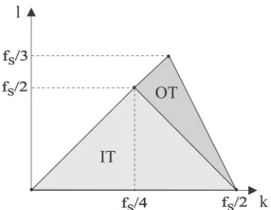
Just as the discrete power spectrum has a point of sym-metry at the folding frequency fs/2, the discrete bispectrum

has many symmetries in the (k,l) plane 关22兴. Because of these, it is necessary to calculate the bispectrum only in the nonredundant region, or principal domain, as shown in Fig. 1. The principal domain can be divided into two triangular regions in which the discrete bispectrum has different prop-erties: the inner triangle 共IT兲 and the outer one关23兴. In the current work it is the IT that is of primary interest. Thus, it is sufficient to calculate the bispectrum over the IT of the prin-cipal domain defined in Refs.关5,7兴: 0⭐l⭐k, k⫹l⭐fs/2.

The bispectrum B(k,l) is a complex quantity, defined by magnitude A and phase␾,

B共k,l兲⫽兩B共k,l兲兩ej⬔B(k,l)⫽Aej␾. 共3兲

Consequently, for each (k,l), its value can be represented as a point in a complex space, Re关B(k,l)兴 versus Im关B(k,l)兴,

thus defining a vector. Its magnitude共length兲is known as the biamplitude. The phase, which for the bispectrum is called the biphase, is determined by the angle between the vector and the positive real axis.

The bispectrum quantifies the relationships among the un-derlying oscillatory components of the observed signals. Specifically, bispectral analysis examines the relationships between the oscillations at two basic frequencies, k and l, and a harmonic component at the frequency k⫹l. This set of three frequencies is known as a triplet (k,l,k⫹l). The bispectrum B(k,l), a quantity incorporating both phase and power information, can be calculated for each triplet.

A high bispectrum value at bifrequency (k,l) indicates that there is at least frequency coupling within the triplet of frequencies k, l, and k⫾l. Strong coupling implies that the oscillatory components at k and l may have a common gen-erator. Such components may synthesize a new component at the combinatorial frequency k⫾l if a quadratic nonlinearity is present.

B. Time-phase bispectral analysis

The classical bispectral method is adequate for studying stationary signals whose frequency content is preserved over time. We now wish to encompass time dependance within the bispectral analysis. In analogy with the short-time Fou-rier transform, we accomplish this by moving a time window w(n) of length M across the signal x(n), calculating the DFT at each window position

X共k,n兲⬵ 1 M n

兺

M⫺1

x共n兲w共n⫺␶兲e⫺j2␲nk/ M. 共4兲

Here, k is the discrete frequency, n the discrete time, and ␶ the time shift. The choice of window length M is a compro-mise between achieving optimal frequency resolution and optimal detection of the time variability. The instantaneous biphase is then calculated: from Eqs.共2兲and共3兲, it is

If the two frequency components k and l are frequency and phase coupled,␾k⫹l⫽␾k⫹␾l, it holds that the biphase is 0

(2␲) radians. For our purposes the phase coupling is less strict because dependent frequency components can be phase delayed. We consider phase coupling to exist if the biphase is constant共but not necessarily⫽0 radians兲for at least several periods of the lowest frequency component. Simultaneously, we observe the instantaneous biamplitude from which it is possible to infer the relative strength of the interaction. We thus hope to be able to observe the presence and persistence of coupling among the oscillators.

III. ANALYSIS

To illustrate the essence of the method, and to test it, we use a generic model of interacting systems whose basic unit is the Poincare´ oscillator:

x˙i⫽⫺xiqi⫺␻iyi⫹gx_i,

y˙_i⫽⫺y_iq_i⫹␻_ix_i⫹g_y

i, 共6兲

qi⫽␣i共

冑

2_⫹

y_i2⫺ai兲.

Here x and y are vectors of the oscillator state variables,␣_i, ai and␻i are constants, and gy( y ) and gx(x) are coupling

vectors. The activity of each subsystem is described by the two state variables x_iand y_i, where i⫽1, . . . ,N denotes the subsystem.

The form of the coupling terms can be adjusted to study different kinds of interaction among the subsystems, e.g., additive linear or quadratic, or parametric frequency modu-lation. Examples will be considered both without and with a zero-mean white Gaussian noise to obtain more realistic con-ditions.

Different cases of interaction are demonstrated for signals generated by the proposed model. In each case we analyze the x1variable of the first oscillator, recorded as a continuous time series. For the first 400 s, the interoscillator coupling strength was zero. It was then raised to a small constant value. After a further 400 s, it was increased again. The first 15 s and corresponding power spectrum for each coupling strength are shown in the figures for each test signal, in order to demonstrate the changes in spectral content and behavior caused by the coupling. For bispectral analysis the whole signal is analyzed as a single entity, but the transients caused by the changes in coupling strength are removed prior to processing. First the classical bispectrum is estimated. Biquencies where peaks provide evidence of possible fre-quency interactions are then further studied by the calcula-tion of the biphase and biamplitude as funccalcula-tions of time. They were calculated using a window of length 100 s, moved across the signal in 0.3 s steps.

A. Linear couplings

Let us start with the simplest case of a linear interaction between coupled oscillators. We suppose model共6兲to consist of only two oscillators, i⫽1,2. The parameters of the model are set to␣1⫽1, a1⫽0.5 and␣2,a2⫽1. The coupling term is unidirectional and linear

gx₁⫽␩2x2, gy₁⫽␩2y2. 共7兲

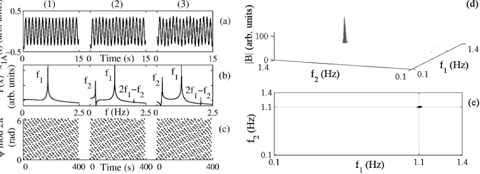
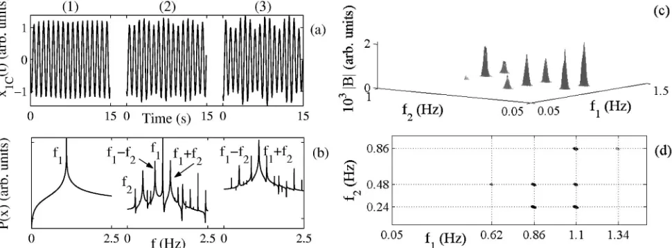
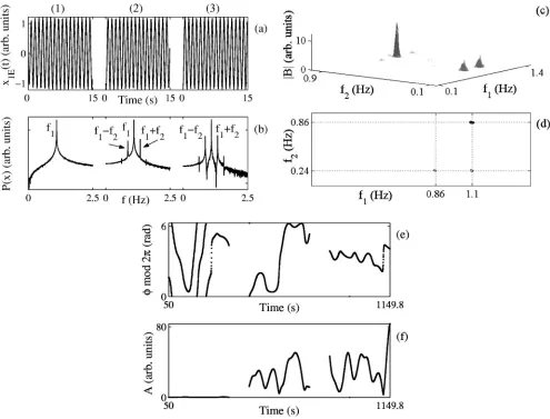
The test signal x1A(t) is the variable x1of the first oscillator. It is presented in Fig. 2共a兲 with the corresponding power spectrum for three different coupling strengths: no coupling ␩2⫽0 and weak couplings␩2⫽0.1,0.2. The peaks labeled as f₁⫽1.1 Hz and f₂⫽0.24 Hz are the independent har-monic components of the first and the second oscillator. These frequencies are deliberately chosen to approximately have a noninteger ratio. There is also at least one peak

FIG. 2. Results in the absence of noise. 共a兲 The test signal x1A(t), variable x1 of the first oscillator with characteristic frequency f1

⫽1.1 Hz. The characteristic frequency of the second oscillator is f2⫽0.24 Hz. The oscillators are unidirectionally and linearly coupled with

three different coupling strengths:␩2⫽0.0共1兲, 0.1共2兲, and 0.2共3兲. Each coupling lasts for 400 s at sampling frequency fs⫽10 Hz. Only the

first 15 s are shown in each case. 共b兲 The power spectrum and共c兲 synchrogram.共d兲 The bispectrum兩B兩, using K⫽33 segments, 66% overlapping, and the Blackman window to reduce leakage and共e兲its contour view.

present at the harmonically related position f₃⫽2 f₁⫺f₂ at-tributable to interaction between the two oscillators. It arises from the nonlinearity of the first oscillator, but is caused by the forcing of the second oscillator.

The principal domain of the bispectrum for the test signal x1A, Fig. 2共d兲, shows one peak at the bifrequency 共1.1 Hz, 1.1 Hz兲, the so-called self-coupling. No other peaks are present. Bispectral analysis examines the relationships be-tween oscillations at the two basic frequencies f1 and f2, and a modulation component at the frequency f1⫾f2, which is absent from the power spectra in Fig. 2共b兲. Therefore, no peak is present at bifrequency 共1.1 Hz,0.24 Hz兲. Thus, the method as it stands is incapable of detecting the presence of linear coupling between the oscillators by analysis of the test signal x_1A. Nonetheless, we still suggest the use of bispec-tral analysis to investigate the presence of nonlinearity, but based on an adapted way of calculating the bispectrum.

In general, the bispectral method can be used to examine phase and frequency relationships at arbitrary time. It is thus well suited for detecting the presence of quadratic couplings and frequency modulation, since they both give rise to fre-quency components at the sum and difference of the inter-acting frequency components.

To be able to detect linear couplings using the bispectral method, as proposed, it is necessary to change the frequency relation. Study of coupled Poincare´ oscillators demonstrate the presence of a component at frequency 2k⫺l as a conse-quence of nonlinearity. This component was detected nu-merically, and is not necessarily characteristic of all nonlin-ear oscillators. By modifying the bispectral definition to

Ba共k,l兲⫽E关X共k兲X共l兲X*共2k⫺l兲兴, 共8兲

the biphase turns into

␾a共k,l兲⫽␾k⫹␾l⫺␾2k⫺l⫺␾c, 共9兲

where index a is introduced and will be used in what follows to indicate that the values are obtained using the adapted method. To obtain 0 radians in the case of phase coupling we have to correct the adapted biphase expression 共9兲 by sub-tracting ␾c⫽2␾l⫺␾k. In the presence of a harmonically

related frequency component and phase coupling, the bi-phase will then be 0 radians.

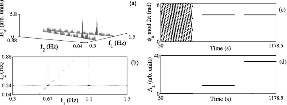
The adapted bispectrum 兩Ba兩 for the signal x_1A exhibits several peaks, as shown in Fig. 3共a兲. It peaks where f1 ⫽f2; a triple product ( f1, f2, f3) of power at frequencies f1 ⫽f2⫽f , and also f3⫽2 f1⫺f2⫽f , raises a high peak at the bifrequency ( f , f ). The self-coupling peak is physically meaningless, and it is therefore cut from the adapted bispec-trum. It can be used for additional checking, since it strongly implies nonlinearity 关6兴.

The peak of primary interest is at bifrequency 共1.1 Hz, 0.24 Hz兲. There is also a high peak positioned at bifrequency

共0.67 Hz,0.24 Hz兲lying on the line where the third frequency in the triplet is equal to the frequency of the first oscillator and is therefore a consequence of the method. The small peaks present in the adapted bispectrum are the result of numerical rounding error and leakage effects due to the DFT calculation.

The peak 共1.1 Hz,0.24 Hz兲 indicates that oscillations at those pairs of frequencies are at least linearly frequency coupled. Frequency coupling alone is sufficient for a peak in the bispectrum to occur. Although the situation can in prin-ciple arise by coincidence, frequency and phase coupling to-gether strongly imply the existence of nonlinearities. To be able to distinguish between different possible couplings, we calculate the adapted biphase Fig. 3共c兲.

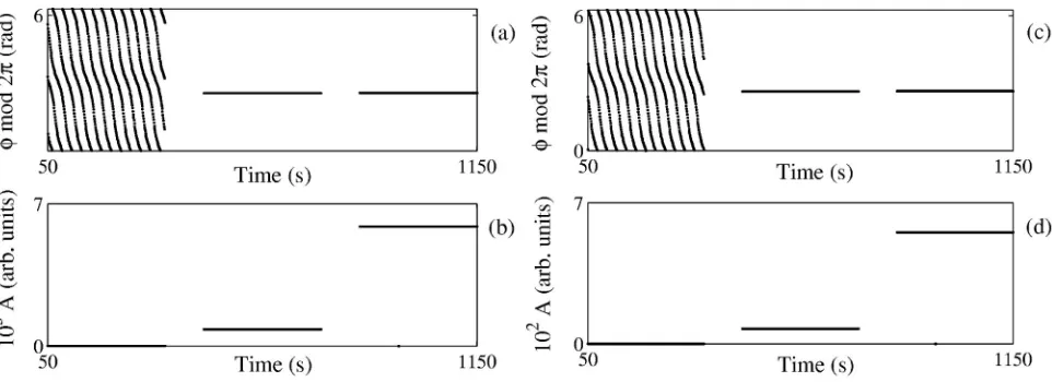
During the first 400 s of test signal x1A, where no cou-pling is present, the adapted biphase changes continuously between 0 and 2␲ radians. For the same time of observation it can be seen that the adapted biamplitude is 0, Fig. 3共d兲. During the second and third 400 s of the signal x1A, a con-stant adapted biphase can be observed indicating the

pres-FIG. 3. 共a兲Adapted bispectrum兩Ba兩, calculated from the test signal x1A using K⫽34 segments, 80% overlapping, and the Blackman

window and共b兲its contour view. Regions of the adapted bispectrum above f2⬎0.88 Hz and below f1⬍0.3 Hz are cut, because the triplets 共1.1 Hz,1.1 Hz,1.1 Hz兲and共0.24 Hz,0.24 Hz,0.24 Hz兲produce high peaks that are physically meaningless.共c兲Adapted biphase␾aand共d兲

ence of linear coupling. The value of the adapted biamplitude is higher in the case of stronger coupling. The coupling con-stant ␩2 can be obtained by normalization, and we are thus able to define the relative strengths of different couplings.

When the oscillators are coupled bidirectionally the fre-quency content of each of them changes and components 2 f1 and 2 f₂ are generated. Both of these characteristic frequen-cies can be observed in the time series of each oscillator. Two combinatorial components are also present in their spec-tra, 2 f1⫺f2 and f1⫺2 f2, assuming that f1⬎f2. In analyz-ing bidirectional couplanalyz-ing, the procedure described above can be extended and two combinatorial components should be analyzed in the same way.

Making use of the calculated instantaneous phases of both oscillatory components we also construct a synchrogram

关Fig. 2共c兲兴, as proposed by Scha¨fer et al.共see Ref.关1兴and the references therein兲, and can immediately establish whether or not the coupling also results in synchronization.

The instantaneous phases can also be used to calculate the direction and strength of coupling, using the methods re-cently introduced by Schreiber, Rosenblum et al., and Palusˇ et al.关2兴.

B. Linear couplings in the presence of noise

We now test the method for the case where noise is added to the variable x₁ of the first oscillator:

x˙1⫽⫺x1q1⫺␻1y1⫹gx₁⫹␰共t兲,

共10兲 y˙₁⫽⫺y₁q₁⫹␻₁x₁⫹g_y

1.

Here ␰(t) is zero-mean white Gaussian noise,

具

典

具

典

FIG. 4. Results in the presence of additive Gaussian noise. 共a兲 Test signal x1B, variable x1 of the first oscillator with characteristic

frequency f1⫽1.1 Hz. The characteristic frequency of the second oscillator is f2⫽0.24 Hz. The oscillators are unidirectionally and linearly

coupled with three different coupling strengths;␩2⫽0.0共1兲, 0.1共2兲, and 0.2共3兲. Each coupling lasts for 400 s at a sampling frequency fs⫽10 Hz. Only first 15 s are shown in each case. 共b兲 Its power spectrum and 共c兲 synchrogram.共d兲Adapted bispectrum 兩Ba兩 using K

⫽33 segments, 66% overlapping, and the Blackman window and共e兲its contour view. The parts of the兩Ba兩 above f2⬎0.79 Hz and below f1⬍0.3 Hz are omitted because the triplets共1.1 Hz,1.1 Hz,1.1 Hz兲and共0.24 Hz,0.24 Hz,0.24 Hz兲produce a high peak that is physically

meaningless. 共f兲 Adapted biphase␾a and 共g兲 adapted biamplitude Aa for bifrequency 共1.1 Hz,0.24 Hz兲, using a 0.3-s time step and a

100-s-long window for estimating the DFT using the Blackman window.

For nonzero coupling strength ␩2, the component at fre-quency position f3 can still be seen in the power spectrum, despite the noise, Fig. 4共b兲. The adapted biphase关Fig. 4共f兲兴 can clearly distinguish between the presence and absence of coupling. When coupling is weaker, the adapted biamplitude

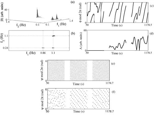
关Fig. 3共g兲兴is lower and the adapted biphase is less constant. The bispectrum for the signal x_1B, shown in Fig. 5共a兲, differs from that in the case of zero noise, Fig. 2共d兲. Noise raises two additional peaks positioned at 共1.1 Hz,0.24 Hz兲 and 共0.86 Hz,0.24 Hz兲. The former could be the result of interaction; the latter is due to the method: the sum of the frequencies in this bifrequency pair gives the frequency of the first oscillator.

Close inspection of the共0.24 Hz,1.1 Hz兲peak by calcula-tion of the biphase gives Fig. 5共c兲. When coupling is present, the characteristic frequency of the second oscillator appears in the power spectrum 关Fig. 4共b兲兴. Two frequencies of high amplitude result in a small peak even if no harmonics are present at the sum and/or difference frequencies. The second

peak is not of interest to us. It can easily be checked whether a phase coupling exists among the bifrequencies from the time evolution of the biphase.

In general, besides estimating bispectral values, one can also observe the time dependences of the phase and ampli-tude for each frequency component and their phase relation-ships. This applies particularly to frequencies that form a bifrequency giving a high peak in the bispectrum or adapted bispectrum. Synchrograms, Figs. 2共c兲and 4共c兲, are obtained by first calculating the instantaneous phase of each oscillator and then their phase difference 关1兴. The phase difference in this case is between two fixed frequencies. We do not calcu-late their instantaneous frequencies, although it is possible to follow the frequency variation by calculating the phase dif-ference at neighboring bifrequencies around the observed one and showing them simultaneously on the same plot. Ex-amples of the phase difference ␺⫽␾1⫺␾2 between the phases of the first␾₁ and the second␾₂ interacting oscilla-tors are shown in Figs. 5共e兲and 5共f兲.

FIG. 5. Bispectrum 兩B兩, calculated from the signal x1B presented in Fig. 4共a兲, using K⫽33 segments, 66% overlapping, and the

Blackman window to reduce leakage and共b兲its contour view.共c兲Biphase␾and共d兲biamplitude A for bifrequency共1.1 Hz,0.24 Hz兲, using a 0.3-s time step and a 100-s-long window for estimating the DFTs using a Blackman window.共e兲Phase difference␺ between␾1of the

characteristic frequency component f1of the first oscillator and␾2of the characteristic frequency component f2of the second oscillator, for

time step 1/fsand共f兲at each period of lowest frequency 1/f2in the bifrequency pair共1.1 Hz,0.24 Hz兲, using interpolation and 100-s-long

C. Quadratic couplings

We now assume that two Poincare´ oscillators can interact with each other nonlinearly. A quadratic nonlinear interaction generates higher harmonic components in addition to the characteristic frequencies 关5兴. In order to study an example where the first f1⫽1.1 Hz and second f2⫽0.24 Hz oscilla-tors are quadratically coupled, we change the coupling terms in model共6兲to quadratic ones

gx₁⫽␩2共x1⫺x2兲2, gy₁⫽␩2共y1⫺y2兲2. 共11兲

Clearly, the test signal x1C presented in Fig. 6共a兲 for three different coupling strengths 关no coupling ␩₂⫽0 共1兲 and weak couplings␩2⫽0.05共2兲,␩2⫽0.1共3兲兴has a richer har-monic structure. In addition to the characteristic frequencies, it contains components with frequencies 2 f1, 2 f2, f1⫹f2, and f1⫺f2 关Fig. 6共b兲兴. Equation 共11兲 also indicates that, as well as having a particular harmonic structure, the compo-nents of the signal x1C also have related phases, 2␾1,2␾2,␾1⫹␾2, and␾1⫺␾2.

We expect several peaks 关24兴to arise in the bispectrum. The peak of principal interest is at bifrequency 共1.1 Hz,0.24 Hz兲. As before, the self-coupling peaks are at共1.1 Hz,1.1 Hz兲 and共0.24 Hz,0.24 Hz兲are of no interest, so they are cut from the bispectrum. Additional peaks appear at the bifrequencies

共0.86 Hz,0.24 Hz兲, 共0.62 Hz,0.48 Hz兲, 共0.86 Hz,0.48 Hz兲,

共1.1 Hz,0.48 Hz兲,共1.1 Hz,0.86 Hz兲, and共1.34 Hz,0.86 Hz兲. The triplet of harmonically related frequency components ( f1, f2, f3) would peak in the bispectrum when the power for all these frequencies differs from zero. The components 0.48 Hz,0.86 Hz,1.34 Hz, and 2.2 Hz resulting from quadratic couplings form such triplets that peak in the bispectrum:

共0.86 Hz,0.24 Hz,1.1 Hz兲,共0.86 Hz,0.48 Hz, 1.34 Hz兲, and

共1.34 Hz,0.86 Hz,2.2 Hz兲. Besides these, there are also other peaks, e.g., that at the bifrequency共0.62 Hz, 0.48 Hz兲arising

from the triplet共0.62 Hz,0.48 Hz,1.1 Hz兲; the sum-difference combination of such frequencies always give the character-istic frequency, or one that results from quadratic coupling. The existence of such peaks has no other meaning than as a strong indicator of second-order nonlinearity. Consequently, the biphase for all peaks due to possible nonlinear mecha-nisms in the bispectrum must have the same value, and same behavior, as shown, e.g., in Figs. 7共a兲and 7共c兲. The biphase is constant in the presence of quadratic coupling. From the biamplitude, the coupling constant can be determined by nor-malization.

In the power spectrum there is a component at frequency 2 f1⫺f2, even although linear coupling is absent. It arises from nonlinearity in the Poincare´ oscillator. The adapted bispectrum for the signal x1C shows a peak at bifrequency

共1.1 Hz,0.24 Hz兲, but the adapted biphase varies continu-ously: we may therefore exclude the possibility of linear cou-pling being present.

D. Quadratic couplings in the presence of noise

As in the case of linear coupling 共Sec. II B兲 we add a noise term to the quadratic coupling g_x

1 and obtain the test

signal x_1D, presented in Fig. 8共a兲.

Using the bispectral and adapted bispectral methods, we find that we obtain results very similar to those in the ab-sence of noise. The method is evidently noise robust. The results for nonzero coupling are quite different from those where coupling is absent, Fig. 8共e兲.

E. Frequency modulation in the presence of noise

We are also interested of being able to detect parametric frequency modulation and to distinguish it from quadratic coupling. Parametric modulation produces frequency compo-nents at the sum and difference of the characteristic

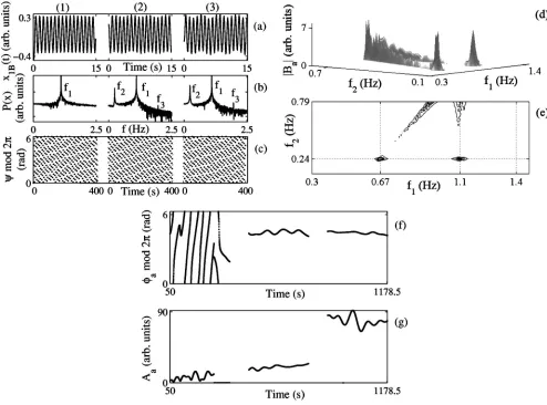
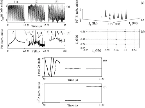
fre-FIG. 6. Results for quadratic coupling in the absence of noise.共a兲The test signal x1C, variable x1of the first oscillator with characteristic

frequency f1⫽1.1 Hz. The characteristic frequency of the second oscillator is f2⫽0.24 Hz. Oscillators are unidirectionally and quadratically

coupled with three different coupling strengths:␩2⫽0.0共1兲, 0.05共2兲, and 0.1共3兲. Each coupling lasts for 400 s at sampling frequency fs

⫽10 Hz. Only the first 15 s are shown in each case.共b兲 The power spectrum. 共c兲 The bispectrum兩B兩, using K⫽33 segments, 66% overlapping, and the Blackman window to reduce leakage and共d兲 its contour view. The part of the bispectrum above f2⬎1.0 Hz is cut,

because triplet共1.1 Hz,1.1 Hz,1.1 Hz兲produces a high peak that is not physically significant.

quency and the modulation frequency, i.e., the same two fre-quency components that can also result from quadratic coupling. Let us now consider an example where the first oscillator f1⫽1.1 Hz is frequency modulated by the second one f2⫽0.24 Hz. For this purpose the equations of the first oscillator become

x˙₁⫽⫺x₁q₁⫺y₁共␻₁⫹␩_mx₂兲⫹␰共t兲,

共12兲

y˙₁⫽⫺y₁q₁⫹x₁共␻₁⫹␩_my₂兲.

The model parameters ␣1,2, a1,2 and the noise intensity D are chosen to be the same as in the previous examples.

We thus obtain a test signal x1E. It is the time evolution of the variable x1of the first oscillator, presented in Fig. 9共a兲 with the corresponding power spectrum 9共b兲for three differ-ent parametric frequency modulation strengths: no modula-tion␩m⫽0; and modulation␩m⫽0.1,0.2. The bispectrum of

the test signal x_1E, Fig. 9共c兲, exhibits several high peaks. The highest are at bifrequencies共1.1 Hz,0.86 Hz兲,共0.86 Hz, 0.24 Hz兲, and共1.1 Hz,0.24 Hz兲, in addition to the共1.1 Hz, 1.1 Hz兲peak. They also appear in the case of quadratic cou-pling. In general, however, the other peaks that appear for quadratic coupling are absent. The reason is that although the component of the second oscillator f2共one component of the triplet兲is not present in the power spectrum, its value is not not exactly zero.

Observing the biphase, no epochs of constant biphase can be observed, although for strong frequency modulation the biphase is less variable. In the power spectrum, Fig. 9共b兲, no component rises above the noise level at frequency f₂, of the bifrequency pair, where the bispectrum peaks. This is an in-dication that there is parametric coupling between the oscil-lators, as there is a high value of biamplitude. The biphase changes runs between 0 and 2␲, and is modulated in the absence of noise. There are also no rapid 2␲ phase slips of the kind that are normal if no modulation is present. In the

absence of couplings and modulation, but in the presence of noise, there would be no such peaks in the power spectrum or bispectrum.

IV. SUMMARY AND CONCLUSIONS

We have extended the bispectral method to encompass time dependence and have demonstrated the potential of the extended technique to determine the type of coupling among interacting nonlinear oscillators. Time-phase couplings can be observed by calculating the bispectrum and adapted bispectrum and by obtaining the time-dependent biphase and biamplitude. The method has the advantage that it allows an arbitrary number of interacting oscillatory processes to be studied.

Recently introduced methods for synchronization analysis among chaotic and noisy oscillations共see Ref.关1兴and refer-ences therein兲 have stimulated applications to a variety of different systems. Methods for quantifying the strength and identifying the direction of couplings, based on nonlinear dynamic or information theory approaches, have recently been proposed关2兴. Here we have addressed the question of the type of coupling that may result in synchronization, and we have proposed a method for its analysis. It is applicable to both univariate data 共a single signal from the coupled system兲 or multivariate data 共a separate signal from each oscillator兲.

Millingen et al. 关15兴 have analyzed multivariate data us-ing a combined wavelet and bispectral method, and have discussed its application in the field of chaos analysis. Here we have concentrated on univariate data and illustrated the potential of the time-phase bispectral method for the detec-tion of higher-order couplings in the presence of noise. The possibility of using univariate data is of particular impor-tance when dealing with real signals, as in practice we often cannot observe and measure the separate subsystems directly, but only their combination, which is intrinsically difficult. Most of the methods proposed so far for synchronization analysis and detection of the direction of couplings are based

FIG. 7. 共a兲The biphase␾ and共b兲 biamplitude A for the test signal x1Cfor bifrequency共1.1 Hz,0.24 Hz兲, using 0.3-s time step and

on bivariate or multivariate data 关1,2兴. In conjunction with frequency or time-frequency filtering 关27兴 or mode decom-position关28兴to obtain two or more ‘‘separate’’ signals, these methods can be used for univariate data as well. Synchroni-zation can also be detected in univariate data through an analysis of angles and radii关29兴in return time maps关30兴.

The time-phase bispectral method proposed in this paper is not only applicable to the synchronization analysis of univariate data but also, at the same time, allows one to determine the nature of the couplings among the interacting nonlinear oscillators. Its benefits include共1兲the possibility of observing the whole frequency domain simultaneously; 共2兲 detecting that two or more subsystems are interacting with each other; 共3兲 quantification of the strength of the interac-tion; and 共4兲determination of whether the coupling is addi-tive linear or quadratic, or parametric in one of the

frequen-cies. We have shown the method to be suitable for the analysis of noisy signals.

Although we have shown that the technique works effec-tively on a well-characterized simple model, there will be some difficulties to be faced and overcome in applying it to real problems, e.g., to data from the cardiovascular system. Understanding the content of the bispectrum and identifica-tion of the peaks of interest are not always straightforward. To appreciate which peaks are those to focus on, one has to be aware of the basic properties of the system and its funda-mental frequencies. Distinguishing a quadratic interaction from parametric frequency modulation may be easy when the coupling 共modulation兲 is relatively strong, but becomes more difficult in the case of relatively weak coupling共 modu-lation兲. In the latter case, observing each phase in the triplet separately can be helpful. Also it is not always an easy task

FIG. 8. Results for quadratic couplings in the presence of additive Gaussian noise. 共a兲 The test signal x1D, variable x1 of the first

oscillator with characteristic frequency f1⫽1.1 Hz. The characteristic frequency of the second oscillator is f2⫽0.24 Hz. The oscillators are

unidirectionally and quadratically coupled with three different coupling strengths:␩2⫽0.0共1兲, 0.05共2兲, and 0.1共3兲. Each coupling lasts for

400 s at a sampling frequency fs⫽10 Hz. Only the first 15 s are shown in each case.共b兲The power spectrum.共c兲The bispectrum兩B兩

calculated with K⫽33 segments, 66% overlapping, and using the Blackman window to reduce leakage and共d兲its contour view. The part of the bispectrum above f2⬎1.0 Hz is cut, because the triplet共1.1 Hz,1.1 Hz,1.1 Hz兲produce a high peak that is physically meaningless.共e兲

The biphase␾and共f兲biamplitude A for bifrequency共1.1 Hz,0.24 Hz兲, with a 0.3-s time step and a 100-s-long window for estimating DFTs using the Blackman window.

to distinguish between quadratic interaction and parametric frequency modulation in the cases when both of them occur simultaneously. Further, where the possible basic frequencies are relatively close, it will be hard to detect them separately. This could cause particular problems in the detection of qua-dratic phase couplings where frequency pairs are close to-gether. Although it is possible in principle to study an arbi-trary number of interacting oscillators, it is advisable in practice to study them in pairs: a knowledge of the basic frequency of each is necessary.

The time-dependent biphase-biamplitude estimate was es-timated with a short-time Fourier transform共STFT兲, using a window of constant length. The optimal window length de-pends, however, on the frequency being studied. The effec-tive length of the window used for each frequency can be varied by applying the wavelet transform, or the selective Fourier transform. For demonstration purposes above, the natural frequencies of the oscillators were chosen to lie

within a relatively narrow frequency interval. A STFT was therefore sufficient for good time and phase 共frequency兲 lo-calization. With a broader frequency content, however, the wavelet transform or selective Fourier transform will need to be applied.

Higher-order spectral methods can be used to study arbi-trary interactions among coupled oscillators: of quadratic, cubic, or even higher order. In this paper we have concen-trated on the lowest one, using the third-order spectrum or bispectrum. For higher orders the volume of the calculations rises substantially, and the method becomes numerically in-creasingly demanding. At the same time, graphical presenta-tion and interpretapresenta-tion of the results become increasingly dif-ficult.

ACKNOWLEDGMENTS

We gratefully acknowledge valuable comments and dis-cussions with Andriy Bandrivskyy, Justin Fackrell, Mounir

FIG. 9. Results for parametric frequency modulation in the presence of additive Gaussian noise.共a兲The test signal x1E, of variable x1

of the first oscillator with characteristic frequency f1⫽1.1 Hz frequency modulated by the second oscillator f2⫽0.24 Hz with three different

frequency modulation strengths: ␩m⫽0.0共1兲, 0.1共2兲, and 0.2共3兲. Each frequency modulation lasts for 400 s, at sampling frequency fs

⫽10 Hz. Only the first 15 s are shown in each case.共b兲The power spectrum.共c兲The bispectrum兩B兩calculated with K⫽33 segments, 66% overlapping, and using the Blackman window to reduce leakage and共d兲its contour view. The part of the bispectrum above f2⬎1.0 Hz is cut,

Ghogho, Fluvio Gini, Georgios B. Giannakis, Peter Husar, Dmitri G. Luchinsky, and Anathram Swami. The study was supported by the Slovenian Ministry of Education, Science and Sport, by INTAS, and by the Engineering and Physical Sciences Research Council共U.K.兲.

APPENDIX: VARIANCE OF THE BISPECTRUM ESTIMATE

In order to interpret bispectral values from a finite length time series, the statistics of bispectrum estimates must be known. To achieve statistical stability, the time series is di-vided into K segments for averaging 关25兴. When there is a large number of segments, the estimate gains statistical sta-bility at the expense of power spectral and bispectral resolu-tion. For a real signal, with a finite number of points, the compromise between bispectral resolution and statistical sta-bility may be expected at K around 30. Estimates are subject to statistical error, such as bias and variance. An estimate must be consistent, that is the statistical error must approach zero in the mean-square sense as the number of realizations becomes infinite. Here we neglect the effects of finite time series length, we assume that they are sufficiently long. Let us consider the bias and the variance of the bispectrum esti-mate Bˆ (k,l). The expected value of Bˆ(k,l) will be

E关Bˆ共k,l兲兴⫽1 K i

兺

K

E关Xi共k兲Xi共l兲Xi*共l,k兲兴

⫽E关X共k兲X共l兲X*共l,k兲兴⫽B共k,l兲, 共A1兲

as K becomes infinite, X_i is the DFT of the ith segment. Thus, Bˆ (k,l) can be taken as an unbiased estimate 关29兴. Its variance will be

var共Bˆ兲⫽E关Bˆ Bˆ*兴⫺E关Bˆ兴E关Bˆ*兴

⫽_K1兵E关兩X共k兲兩2兩X共l兲兩2兩X共k⫹l兲兩2兴⫺E兩B共k,l兲兩2其.

共A2兲

Note that the variance is inversely proportional to K. From a mathematical statistics point of view, it is a nontrivial task to compute the quantity in the bracket in terms of low order spectra, but one may write a good approximation关26兴,

E关兩X共k兲兩2兩X共l兲兩2兩X共k⫹l兲兩2兴⫽P共k兲P共l兲P共k⫹l兲,

共A3兲

in which case the variance will be

var共Bˆ兲⫽E关兩Bˆ共k,l兲兩2兴⫺E关Bˆ共k,l兲兴2

⬇1

KP共k兲P共l兲P共k⫹l兲关1⫺b

2_{共k,l兲兴. 共A4兲}

Note that it is a consistent estimate in the sense that the variance approaches zero as K becomes infinite. The vari-ance is proportional to the product of the powers †P(k) ⫽E关X(k)X*(k)兴‡ at the frequencies k, l, and k⫹l. Conse-quently, a larger statistical variability is introduced in esti-mating larger values in the bispectrum. Finally, the variance is proportional to关1⫺b2_{(k,l)兴, where the bicoherence b}2 _is a normalized bispectrum, b2(k,l)⫽E关Bˆ (k,l)兴2/

关P(k) P(l) P(k⫹l)兴. That is, when the oscillations at k, l, and k⫹l are nonlinearly coupled (b2⬇1), the variance ap-proaches zero, and when the components are statistically in-dependent (b2⬇0), the variance is proportional to the power at each spectral component 关26兴.

Brillinger and Rosenblatt 关3兴 have investigated the asymptotic mean and variance of Fourier-type estimates of high-order spectra and proved that under certain assumptions the kth order spectral estimate is asymptotically unbiased and Gaussianly distributed and that estimates of different or-der are asymptotically independent. The variances of the real and imaginary parts of the bispectrum are asymptotically

共i.e., for large K) Gaussian and are equal, var兵Re关Bˆ (k,l)兴其

⬵var兵Im关Bˆ (k,l)兴其. For a perfect phase-coupled triplet, the variances of the real and imaginary parts are equal to zero. In the case of no coupling, there is an identical contribution to the variances from the real and imaginary parts of the esti-mate of the bispectrum.

The total variance is a sum of individual (i⫽1, . . . ,K) contributions, because different triplets are mutually statisti-cally uncorrelated in the absence of phase coupling. Partial coupling can be expected to result in a combination of per-fectly phase-coupled oscillations and oscillations with ran-domly changing phases.

关1兴A.S. Pikovsky, M.G. Rosenblum, and J. Kurths,

Synchroniza-tion; A Universal Concept in Nonlinear Sciences共Cambridge University Press, Cambridge, 2001兲.

关2兴T. Schreiber, Phys. Rev. Lett. 85, 461共2000兲; M.G. Rosenblum and A.S. Pikovsky, Phys. Rev. E 64, 045202 共2001兲; M.G. Rosenblum, L. Cimponeriu, A. Bezerianos, A. Patzak, and R. Mrowka, ibid. 65, 041909 共2002兲; M. Palusˇ, V. Koma´rek, Z. Hrncˇı´rˇ, and K. Sˇteˇbrova´, ibid. 63, 046211共2001兲.

关3兴D.R. Brillinger and M. Rosenblatt, Spectral Analysis of Time

Series共Wiley, New York, 1967兲.

关4兴A. Swami, G.B. Giannakis, and G. Zhou, Signal Process. 60, 65共1997兲.

关5兴C.L. Nikias and A.P. Petropulu, Higher-Order Spectra Anlysis:

A Nonlinear Signal Processing Framework 共Prentice-Hall, Englewood Cliffs, 1993兲.

关6兴G. Zhou and G.B. Giannakis, IEEE Trans. Signal Process. 43, 1173共1995兲.

关7兴J.W.A. Fackrell, Ph.D. thesis, University of Edinburgh, 1996

共unpublished兲.

关8兴Y.C. Kim, J.M. Beall, E.J. Powers, and R.W. Miksad, Phys.

Lett. 74, 395共1995兲; B.Ph. van Milligen et al., Phys. Plasmas

2, 3017共1995兲.

关16兴J. Jamsˇek, M.Sc. thesis, University of Ljubljana, 2000.

关17兴A. Stefanovska and M. Bracˇicˇ, Contemp. Phys. 40, 31共1999兲.

关18兴J.M. Mendel, Proc. IEEE 79, 278共1991兲.

关19兴A.K. Nadi, IEE Proc. F, Commun. Radar Signal Process. 140, 380共1993兲.

关20兴A.K. Nadi, Higher-Order Statistics in Signal Processing

共Cambridge University Press, Cambridge, 1998兲.

Volkmann, A. Schnitzler, and H.-J. Freund, Phys. Rev. Lett.

81, 3291共1998兲; A. Stefanovska and M. Hozˇicˇ, Prog. Theor. Phys. Suppl. 139, 270共2000兲.

关28兴N.E. Huang, Z. Shen, S.R. Long, M.C. Wu, H.H. Shih, Q. Zheng, N. Yen, C.C. Tung, and H.H. Liu, Proc. R. Soc. Lon-don, Ser. A 454, 903共1998兲.

关29兴N.B. Janson, A.G. Balanov, V.S. Anishchenko, and P.V.E. Mc-Clintock, Phys. Rev. E 65, 036211共2002兲.