Data based mechanistic modelling, forecasting, and control

(1)

SPECIAL SECTION

By Peter Young and Arun Chotai

I

n the environmental and agricultural sciences, as in many

ar-eas of engineering and science, mathematical models are

nor-mally formulated as deterministic differential (or equivalent

discrete-time) equations. Most often, the structure of these

equations is defined by the scientist or engineer in a form that

is perceived to be appropriate according to the physical

na-ture of the system and the current scientific paradigms in the area of

study. Most of the “simulation” models that emerge from this

ap-proach are very large, with many unknown parameters.

Conse-quently, they are difficult, if not impossible, to identify, estimate, and

validate in rigorous statistical terms because of problems associated

with over-parametrization and the lack of experimental or monitored

data. Unlike the situation in engineering, however, natural

environ-mental systems, and many systems in agriculture, are not normally

Young ([email protected]) and Chotai are with the Centre for Research

on Environmental Systems and Statistics, Institute of Environmental and

Natu-ral Sciences, Lancaster University, Lancaster LA1 4YQ, U.K.

21st

CENTURY

(2)

manmade. As a result, their internal physical, biological,

and ecological mechanisms are often poorly understood,

and planned experiments that might lead to improvements

in such understanding are either difficult or, in the case of

environmental systems, even impossible to undertake.

Increasingly in recent years, however, the poorly defined

nature of many environmental and agricultural systems has

been recognized. It is now becoming accepted that a new

modeling philosophy and associated methodology is

re-quired that acknowledges the need to quantify the

uncer-tainty associated with the model (e.g., [1]-[3]). The Centre for

Research on Environmental Systems and Statistics (CRES) at

Lancaster University has been prominent in this area of

re-search. This article outlines the major aspects of our

ap-proach to stochastic modeling, as well as briefly describing

three studies that demonstrate the practical utility of this

ap-proach. In particular, the article shows how parametrically

efficient (parsimonious), low-order stochastic models can be

produced that reflect the dominant modal characteristics of

the system and can be interpreted in physically meaningful

terms. Within the present context, the most important aspect

of these data-based mechanistic (DBM) models is that they

provide an appropriate basis for advanced nonstationary or

nonlinear signal processing, adaptive forecasting, and

multivariable control system design.

Unlike data-based “black-box” models, DBM models are

required to have a mechanistic interpretation. Indeed, they

are not deemed truly credible in scientific terms unless such

an interpretation proves possible. But, unlike the situation

with “grey-box” models, such a physically meaningful

expla-nation is not imposed as a hypothesis prior to modeling.

Rather, it emerges from an inductive modeling procedure

only after the model structure has first been identified

parsi-moniously from a generic class of models with wide

applica-tion potential. In this manner, prior scientific prejudice

about the nature and complexity of the model is avoided,

and the resulting DBM model will normally have a structure

and parametrization that is appropriate to the information

content of the data. In this article, the generic class of

mod-els used in DBM modeling comprises stochastic linear and

nonlinear differential or difference equations, or their

trans-fer function equivalents.

DBM modeling methods were developed originally for

the analysis of measured time-series data, particularly in

re-lation to the design of signal processing, forecasting, and

au-tomatic control systems. In the early stages of modeling,

when observational data are either scarce or not available,

however, the same methodological tools can also be used to

obtain reduced-order versions of the large simulation

mod-els. The importance of reduced-order models that reflect

the dominant modes of system behavior is being widely

rec-ognized in many areas of application within the

environmen-tal and agricultural sciences. For example, such models

have been used in the simplification of large simulation

models used in climate research (e.g., [4]) and in optimal

control system design (e.g., [5]). An example of the DBM

ap-proach to model reduction is the modeling and control of

the microclimate in a large horticultural greenhouse [6]

where the reduced-order control model is obtained from a

much larger nonlinear simulation model. A similar DBM

ap-proach has been used to obtain linear, reduced-order

ver-sions of the topically important “global carbon cycle”

models [6], [7] used in the studies of the International Panel

on Climate Change (IPCC).

This article outlines the main aspects of DBM modeling,

as well as the associated methods of signal processing,

adaptive forecasting, and multivariable control that exploit

such models. This overall generic approach appears to have

wide application potential, and its practical utility is

illus-Table of Abbreviations

AMV Active mixing volume

AR Autoregressive (model)

ARC Adaptive radar calibration (system) R_T2 _{Coefficient of determination based on}

simulation response error

CRES Centre for Research on Environmental Systems and Statistics

CV Control volume

DBM Data-based mechanistic DMA Dominant mode analysis

FIS Fixed-interval smoothing

GPC Generalized predictive control

GSA Generalized sensitivity analysis HMC Hybrid-metric-conceptual (model)

IPCC International Panel on Climate Change

KF Kalman filter LQ Linear quadratic

LQG Linear quadratic Gaussian

MFD Matrix fraction description MCS Monte Carlo simulation

NMSS Nonminimal state space

PDF Probability distribution function

PIP Proportional-integral-plus (controller) RLS Recursive least-squares (method)

RIV Refined instrumental variable (method)

SRI Silsoe Research Institute

SDP State-dependent parameter (model)

SVF State variable feedback (control)

SRIV Simplified refined instrumental variable (method)

TF Transfer function (model) TVP Time-variable parameter (model)

[image:2.612.317.551.59.545.2]

(3)

trated by three practical examples. These range from the

model reduction and control application mentioned above

through the modeling and control of forced ventilation

sys-tems in agricultural buildings to the design of adaptive flood

forecasting and warning systems.

Methodological Background

The methods used in this article have been developed over

the past 20 years, and they cover four main areas: DBM

methods for modeling linear and nonlinear stochastic

sys-tems; dominant mode analysis (DMA) leading to the

com-bined linearization and simplification of large simulation

models; unobserved component (UC) models and their use

in the recursive estimation, forecasting, and smoothing of

nonstationary time series; and nonminimal state space

(NMSS) methods of control system design. All of these

meth-ods have been described in detail elsewhere, so they are

outlined only briefly in the following subsections.

Data-Based Mechanistic Modeling

Previous publications (e.g., [6]-[10]) illustrate the evolution

of the DBM philosophy and its methodological

underpin-ning. This methodological basis is heavily dependent on the

exploitation of recursive estimation in all its forms. These

include the traditional application to online and offline

pa-rameter estimation using recursive least-squares (RLS) and

optimal refined instrumental variable (RIV) algorithms; the

design of adaptive forecasting systems using the Kalman

fil-ter (KF) algorithm; the use of recursive fixed-infil-terval

smoothing (FIS) for more statistically efficient, offline

time-variable parameter (TVP) estimation for use in signal

extraction; and the exploitation of FIS combined with other

procedures for state-dependent parameter (SDP)

estima-tion and the nonparametric/parametric identificaestima-tion of

nonlinear stochastic systems.

The three major phases in the DBM modeling strategy

are as follows:

• Stochastic Simulation Modeling and Sensitivity Analysis

(e.g., [2], [3], [6], [8], and the references therein). In

the initial phases of modeling, observational data may

well be scarce, so any major modeling effort will have

to be centered on simulation modeling, usually based

initially on largely deterministic concepts such as

dy-namic mass and energy conservation. Recognizing

the inherent uncertainty in many environmental and

agricultural systems, however, these deterministic

simulation equations can be converted into an

alter-native stochastic form. Here, it is assumed that the

as-sociated parameters and inputs can be represented in

some suitable stochastic form such as a probability

distribution function (PDF) for the parameters and

time-series models for the inputs. The subsequent

stochastic analysis then exploits Monte Carlo

simula-tion (MCS) in three ways: first, to explore the

propaga-tion of uncertainty in the resulting stochastic model;

second, as a mechanism for generalized sensitivity

analysis (GSA) to identify the most important

parame-ters leading to a specified model behavior; and third,

the use of MCS in stochastic optimization.

• Dominant Mode Analysis and Simulation Model

Simpli-fication

(e.g., [6], [7], and the references therein). The

initial exploration of the simulation model in

stochas-tic terms can reveal the relative importance of

differ-ent parts of the model in explaining the dominant

behavioral mechanisms. This understanding of the

model is further enhanced by employing a novel

method of combined statistical linearization and

model order reduction. This is applied to time-series

data obtained from planned experimentation, not on

the system itself, but on the simulation model that

be-comes a surrogate for the real system. Such DMA is

ex-ploited to develop low-order, dominant mode

approximations of the simulation model;

approxima-tions that are often able to explain its dynamic

re-sponse characteristics to a remarkably accurate

degree (e.g., coefficients of determination

>

0.999; i.e.,

greater than 99.9% of the high-order model output is

explained by the low-order model). Conveniently, the

statistical methods used for such linearization and

or-der reduction exercises are the same as those used for

the next phase in the modeling process.

(4)

esti-mation [12]-[14], whereas if the system is heavily

nonlinear, the SDP estimation allows for identification

of the nonlinear model structure prior to final

nonlin-ear parametric estimation (see [7], [9], [14]). This

lat-ter approach provides an allat-ternative to, or a

reinforcement of, other approaches to nonlinear

mod-eling, such as neural network and neuro-fuzzy

model-ing (e.g., [15]). It has the advantage that the resultmodel-ing

models are normally much less complex, of

consider-ably lower order, and more easily interpretable in

mechanistic terms.

DBM modeling is obviously very different from

physi-cally based simulation modeling, but it is often confused

with grey-box modeling. Grey-box modeling follows the

tra-ditional hypothetico-deductive approach. Here the

hypoth-esis is normally in the form of a much-simplified model of

the physical system under study, and deduction is based on

estimating the parameters that characterize this assumed

model structure from measured data. In contrast, DBM

mod-eling is inductive and commences with few prior

percep-tions of the model form, except that it is a member of a

suitable, generic class of models (normally linear/nonlinear

differential equations or their discrete-time equivalents).

Methods of statistical model structure identification and

pa-rameter estimation are then utilized to produce a

low-di-mensional, black-box model, within this generic class of

models, that explains the data unambiguously in a

statisti-cally efficient manner. Only then is the question of the

un-derlying, mechanistic interpretation of the model

addressed, as illustrated by the examples discussed later. In

this manner, a minimally parametrized and statistically

well-defined model is obtained, and the dangers of imposing

too much confidence in prior assumptions about the

physi-cal nature of the system are avoided.

Signal Processing, Forecasting,

and Automatic Control

The DBM methods were developed primarily for modeling

systems from normal observational time-series data

ob-tained from monitoring exercises (or planned

experimen-tation, if possible) carried out on the real system. Often,

such time series require some form of preprocessing, and

this is accomplished using methods of nonstationary

time-series analysis based on recursive fixed-interval

smoothing (e.g., [11], [12], and the references therein).

These powerful statistical tools allow for interpolation

over gaps in the time series; the detection of outliers;

“sig-nal extraction,” including the estimation and removal of

periodic components (e.g., seasonal adjustment); and

time-frequency analysis.

The DBM models are also in a form appropriate for

model-based forecasting and control system design. Of

course, any available methods can be used for these

appli-cations. At Lancaster, however, the stochastic UC

model-ing approach based on TVP estimation provides the main

vehicle for adaptive forecasting ([12], [13], and the

references therein). Model-based automatic control

sys-tem design is formulated within the NMSS setting, normally

resulting in the multivariable proportional-integral-plus

(PIP) control algorithm (see [16] and the references

therein). The NMSS is the most natural state-space

defini-tion for discrete-time transfer funcdefini-tion models, and the PIP

controller provides a natural multivariable extension of

the conventional PI and PID controllers. In addition to

pro-portional and integral action, it includes additional

for-ward path and feedback filters that allow for NMSS state

feedback, without the need for state reconstruction, thus

enhancing robustness and closed-loop performance. Of

course, the PIP controller is just one specific outcome of

the NMSS design concept. This concept is not only

attrac-tive in its own right, but control algorithms that derive

from it are very general in form and thus able to mimic

other well-known design procedures, such as minimal

state linear quadratic Gaussian (LQG), generalized

predic-tive control (GPC), and Smith predictor control for

time-de-lay systems (see [17] and the references therein).

It should be noted that many of the time-series analysis

and modeling procedures mentioned above and used in

the examples described below are contained in the

MATLAB

CAPTAIN

time-series analysis and forecasting

toolbox, currently in the final stages of beta testing (see

http://www.es.lancs.ac.uk/cres/captain/).

Modeling and Control of a

Greenhouse Microclimate

The literature on modeling of the microclimate in

green-houses is very large, with models ranging from high-order,

nonlinear simulation models (e.g., [18]) through much

sim-pler but still physically meaningful data-based models (e.g.,

[19]) to purely black-box models (e.g., [5]). One important

aspect of this research has been the development and use of

models for the control of greenhouse microclimates (e.g.,

[20] and the references therein). This example falls into the

latter category and is concerned with the modeling and

au-tomatic control of the microclimate in the large Venlo

horti-cultural greenhouse at the Silsoe Research Institute (SRI) in

Bedford, U.K.

(5)

To simplify the model shown in Fig. 1, it was perturbed

about a number of different operating points by suitably

de-signed input functions. These were applied to each control

input in turn (i.e., the fractional valve aperture of the

heat-ing boiler

u

_1,_t

, the input to the mist spraying system

u

_2,_t

, and

the CO

2

enrichment input

u

3,t

), and they produced climate

perturbations defined by the internal air temperature

y

_1,_t

in

°C, the percentage relative humidity

y

2,t

, and the CO

2

con-centration

y

3,t

in ppm. The input-output perturbational data

set obtained in this manner was then used as the basis for

the identification and estimation of reduced-order,

dis-crete-time linear models that were directly suitable for

model-based PIP system design [21].

At the most important operating condition, the

esti-mated reduced-order model for

y

t t t t

T

y

=

[

1, 2, 3,

]

, in

re-sponse to

u

t t t t

T

u

=

[

1, 2, 3,

]

, takes the form of the

following discrete-time, transfer function matrix model:

y

t

z

=

−

− −

−

0 0143

1 0 9056

0 0712

0 0 0587

1 0 79

1

.

06 0 7909

0

0 01791

1 0 6996

831294

1 0

1

z

−

.

.6541

1

z

t

−













u

.

(1)

CO2

Humidity

Air Temperature

1/s

1/s ×1

×2

×3

×4

×5

×6

×7

×8

×9

×10

×11 Weather

Inputs

Control Inputs

Thermal Rad Coeffs

Heat Trans Coeffs

Stomatal Res

CO Model2

Latent Heat En Ex En Ex

Derivatives Demux

Mux u1

u2

u3

u4

u5

u6

u7

u8

(6)

This model is well identified, and the parameter estimates

are statistically well defined. As might be expected, the

ma-jor coupling is between the temperature and relative

humid-ity, with CO

2

being almost independent of these variables.

Despite its simplicity, the model explains the high-order

nonlinear model response very well, with coefficients of

de-termination

R

_T2

0 99

>

.

(i.e., over 99% of the high-order model

response explained by the low-order model). Clearly, the

dominant modal behavior of the simulation model at this

operating condition, which is so important for subsequent

control system design, has been captured very well.

More-over, this model is much simpler than might be expected on

the basis of the full nonlinear model equations.

From the DBM standpoint, it is important that the

re-duced-order model should make good physical sense, and,

as expected from mass and energy transfer considerations,

the temperature and humidity dynamics are highly coupled.

Indeed, it is possible to associate the model (1) with the

dif-ferential equations of mass and energy transfer for this

sys-tem (much simplified versions of the equations used to

derive the high-order model in Fig. 1). Since the model is

es-timated in discrete time, however, this relationship is not

too transparent. Consequently, it is better to delay our

illus-tration of such a mechanistic interpretation to the next

sec-tion, where a related model is estimated directly in

continuous-time terms and the physical interpretation is

much more obvious.

The high-order simulation model provided a very

use-ful vehicle for initial PIP control system design and

evalu-ation exercises [21], where it functioned as a valuable

surrogate for the real system before experimentation

was possible. Furthermore, the fact that the

reduced-or-der models were

structurally

identical to those identified

later from the real data meant that the initial PIP

control-ler designs were also structurally similar. Note that the

inherent stochastic nature of the DBM models is most

im-portant in the PIP control system design process, since it

allows for evaluation of the controller’s robustness to

uncertainty using stochastic simulations. These can be

either single simulations with stochastic inputs or MCS

used to assess the robustness of the control system to

uncertainty in the model parameters (e.g., [17] and the

references therein).

NMSS control system design is straightforward and

flexi-ble in this example [21]. Once the reduced-order TF matrix

model (1) has been obtained, it is converted

straightfor-wardly to the left matrix fraction description (MFD), and

thence to the following NMSS form:

x

t+1

=

Fx

t

+

Gu

t

+

Dy

d t, +1

y

t

=

Hx

t

(2)

where

F

and

u

t

are defined as at the bottom of the next page

and

G

=

−

0 0143

0 0712

0 0 0587

0 7909

0

0 01791

831294

0

0 .

.

0

1

0

1

0

1 0 0143

0 0712

0 0 0587

0 7909

0

0 01791

8 −

−

.

31294

.













H

=













1 0 0 0 0 0 0 0 0 0 0 0

0 1 0 0 0 0 0 0 0 0 0 0

0 0 1 0 0 0 0 0 0 0 0 0

D

=













0 0 0 0 0 0 0 0 0 1 0 0

0 0 0 0 0 0 0 0 0 0 1 0

0 0 0 0 0 0 0 0 0 0 0 1

T

.

Here

x

t

=

[

y

1,t

y

2,t

y

3,t

y

1,t−1

y

2,t−1

y

3,t−1

u

1,t−1

u

2,t−1

u

3,t−1

z

t

z

t

z

t

T

1, 2, 3,

] is the NMSS vector;

u

t

u

t

u

t

u

t T

=

[

1, 2, 3,

]

is the

control input vector; and

y

d t d t d t d t

T

y

,

=

[

1, 2, 3,

]

is the

com-mand input vector (the user-defined levels of the three

cli-m a t e v a r i a b l e s ) . T h e v a r i a b l e s

z

i t,

,

i

=

1 2 3 a re

, ,

integral-of-error states, introduced to ensure type 1

servo-mechanism performance (unity gain to the command inputs

and steady-state decoupling: i.e., in the steady state, the

controlled variables all reach their demand levels without

any effect on the steady-state levels of the other output

vari-ables).

PIP control system designs based on this NMSS model (2)

provide the basis for any SVF design procedures, such as

op-timal linear-quadratic (LQ), pole assignment, or

risk-sensi-tive/robust design. In the simplest LQ case, for example,

quadratic

cost

function

weighting

matrices

Q

=

diag[

111111111 100 5 25

]

and

R

=

diag [

1 01 01

.

. ]

produce the SVF control law below (equation

u

t

at the bottom

of the next page), where the off-diagonals of the last 3

×

3 block in the matrix have been constrained to zero

consis-tent with the steady-state decoupling requirement. Note

that the pair [ , ]

F G

is stabilizable by the nonminimal state

feedback, and, in addition, we can always find a matrix

E

such that the Cholesky decomposition

EE

T

Q

=

, ensuring

that the pair [ , ]

F E

is observable [22]. Consequently, this

PIP-controlled system will be stable and achieve the desired

LQ optimality.

(7)

that the relative values of the cost function weighting

ma-trix elements associated with the three integral-of-error

states have been adjusted here to ensure that the rise

times of each channel have the required control

character-istics, while minimizing harsh actuator movements that

could cause wear.

The controller designed in the above manner was

vali-dated in practical terms over a three-month implementation

period during the 1993-1994 growing season with a tomato

crop in the greenhouse. Fig. 3 shows the control

perfor-mance of each climate variable over the entire validation

pe-riod. Each graph shows the percentage of the validation

period that a control variable was inside a certain control

limit. For example, air temperature was less than 1°C away

from the set point for 98% of the validation period. This

per-formance easily meets the requirements of the growers.

Finally, it should be noted that the results shown in Figs. 2

and 3 were obtained with the simple, constant-gain,

multivariable controller defined above, and some

improve-ments in performance would be possible if more complex

control systems were used. For

exam-ple, further decoupling of the

tempera-ture and humidity control can be

accomplished by exploiting a special

form of multiobjective optimization

de-veloped at Lancaster (e.g., [16]). Here,

the Cholesky factors of the LQ cost

function weighting function matrices

are optimized so that off-diagonal

weightings are introduced into the cost

function to ensure satisfactory

de-coupling (or other multiobjective

re-quirements).

The responses obtained with such

an optimized PIP controller are shown

as the thick lines in Fig. 2; clearly, almost perfect decoupling

has been achieved. Other possible improvements include a

stability-guaranteed, neuro-fuzzy gain scheduling system

F

=

−

0 9056

0

0 0 0

0

0 0 0645

0 0 0 0

0 0 7906

0 0 0

0

0 0 6253

0 0 0 0

0

1 .

.

3537

0 0

0 4576 0

.

01171

.

581536 0 0 0

.

1

0

0 0 0

0

0 0 0 0

0

1

0 0 0

0 −

−

0

0 0 0 0

0

1 0 0

0

0 0 0 0

0

0 0 0

0

0 0 0 0

0

0 0 0

0

0 0 0 0

0

0 0 0

0

0 0 0 0

0 9056

0

0 0 0

0

0 0 0645

0 1 0 0

0 0 7906

0 0 0

0

0 0 6253

0 0 1

−

.

0

0 −

13573 0 0

0 4576

0 −

01171

581536

0 0 1







.









u

t

= −

−

22 8406 12938

0 0 0

0

0 0 6036

0 0001

5 6927

0

0 0 6954

0 .

.

9666

0 0 0

0

0 0 7149

0 0001

0 0 7991

0 0 0015

0 0021 0 0021

−

0 0

−

0 0055 0

−

0 0001

−

0 6996

0

0 −

0 0112













.

x

t

Temperature Humidity Carbon Dioxide

[ C]° [% RH] [p/m]

100 100 100

75 75 75

50 50 50

25 25 25

0 0 0

[%

Time]

[%

Time]

[%

Time]

0 0.5 1 1.5 0 2 4 6 0 20 40 60

Figure 3.

Long-term controller performance for the SRI Venlo greenhouse; presented as

percentage of total evaluation period (% time) against absolute control error in relation to

the set point (control limit).

u1 to y1

u1 to y2 u2 to y2

u2 to y1 1.5

1

0.5

0

−0.5 −1 −1.5

0 20 40

0

−0.05

−0.1

0 20 40

1.5

1

0.5

0

0 20 40

(8)

(e.g., [23]) or a fully adaptive PIP control system (e.g., [24]).

The latter would be straightforward to implement, since the

recursive estimation algorithms used in the modeling stage

of the design can be easily implemented online in real time.

However, the performance shown in Fig. 3 is perfectly

ac-ceptable for most practical purposes, and such added

com-plexity is not warranted in this case.

Modeling and Control

of Forced Ventilation Systems

This example is related to the previous one and concerns the

analysis of data from planned experiments in a large

instru-mented chamber in the Laboratory for Agricultural Buildings

Research at the Katholieke Universiteit Leuven (for details,

see [25]). This chamber, shown in Fig. 4, has a volume of 9 m

3

and has been designed to represent a scale model of a

live-stock building or greenhouse for use in experimental

re-search on forced ventilation and heating in agricultural

buildings. The two variable inputs, ventilation rate (120-300

m

3

/h) and heating element input (0-400 W), determine the

dominant airflow pattern within the chamber. An envelope

chamber or “buffer zone” is constructed around the test

room to minimize disturbance of the airflow by heat

conduc-tion from the laboratory. A series of aluminum conductor

heat sinks and steam generation from a water reservoir

pro-vide the internal heat and moisture production to simulate

animal occupants. To gain information about the distribution

of mass and energy in a quantitative manner, 36 temperature

sensors and 24 humidity sensors are positioned in a

three-di-mensional (3-D) array within the chamber.

The agricultural engineering literature reports a great deal

of research on the modeling of ventilated air spaces, much of

it based on deterministic simulation models. More recent

data-based modeling has been stimulated by the control

vol-ume (CV) concept of Barber and Ogilvie [26]. For example,

Berckmans et al. [25] use least-squares methods to estimate

the parameters in a simple conceptual CV model of an

imper-fectly mixed 3-D airspace from variations in ventilation rate

and heat supply, whereas Daskalov [27] develops a model for

measured temperature and humidity variations in a naturally

ventilated pig building using discrete-time TF models. To

ob-tain the DBM model, which can be considered a natural

ex-tension of these earlier models, the continuous-time SRIV

estimation algorithm is used first to identify the linear TF

(or-dinary differential equation) model between the measured

temperatures at the inlet,

T

_i

, and the outlet,

T. In the case of

the response to a step increase of the ventilation rate from 80

to 300 m

3

/h, the estimated model for the change in

tempera-ture

∆

T

from the initial steady levels takes the form

∆

T t

s

∆

s

T t

i t

( )

.

( )

=

+

1959

0 089

2962

0111

2

ξ

(3)

where

s

is the differential operator and

ξt

is the residual

noise. Fig. 5 compares the output of this model with the

mea-sured change in the outlet temperature, and the associated

residual

ξt

is plotted in the lower graph. This unexplained

residual has a zero mean value and low variance (0.021

com-pared with a measured variance of 2.619 for the output

∆

T

series;

R

T

2

0 992

=

.

).

The TF model can be decomposed into a parallel or

feed-back connection of first-order processes, but the latter has

more physical significance, as required in DBM modeling.

This becomes clear if we invoke the classical theory of heat

transfer and formulate the differential equations of dynamic

heat transfer, bearing in mind the need to arrive at a

sec-ond-order, lumped, differential equation with a TF similar to

(3). Such analysis [28] yields the following equations for the

main chamber and the buffer zone:

Main Chamber:

d

T

dt

T

i

K

T

(

∆

)

∆

=

β

1

+

1 buff

−

α

1

Buffer Zone:

d

T

dt

K

T

K

T

(

)

(

)

∆

buff

_∆

buff buff

= −

2

+

3

−

.

In these equations,

β

1 1

=

V

vol

;

α

1 1

γ

1 1

1 1 1

=



+





_vol

V

_vol

k

sf

_cp



_



;

K

1

k

1 1

1 1 1

=

sf

vol

γ

cp

;

K

₂

k

2 2 2 1 1

=

sf

vol

γ

cp

and

K

₃

k

1 1 2 1 1

=

sf

vol

γ

cp

[image:8.612.312.552.529.709.2]

where

T

is the temperature (°C) measured at the outlet

port but assumed to be representative of the temperature

in the active mixing volume (AMV) [10];T

i

is the temperature

(9)

(°C) measured at the chamber inlet;

V

is the ventilation rate

(m s

3 −1

_);

_γ

1

is the air density of the incoming air and the air in

the main chamber (kgm

−3

_);cp1

_{is the specific heat capacity of}

the incoming air (Jkg

-1

C

-1

°

) and the air in the main

cham-ber;

k

1

is the thermal conduction coefficient through the

in-ner chamber walls (Wm

−2

_°

C

−1

_{); sf}

1

is the surface area of the

AMV for imperfect mixing (m

2

);

T

buff

is the temperature in

the outer buffer zone (°C); vol2

is the volume of the AMV

as-sociated with the buffer zone (m

3

);

k

2

is the thermal

con-duction coefficient through the buffer zone (outer

chamber) wall (Wm

−2

_°

C

−1

_{); and sf2}

_{is the surface area of the}

buffer zone AMV for imperfect mixing (m

2

).

The differential equations above may be combined and

expressed in TF form to yield the following second-order TF

model for the complete chamber-buffer zone system:

∆

T

b s

b

∆

s

a s

a

T

i

=

+

0 1

2

1 2

(4)

where

b

0

= β

1

;

b

1

=

β

1

(

K

2

+

K

3

);

a

1

=

(

K

2

+

K

3

+ α

1

)

;

a

2

=

(

K

2

+

K

3

)

α

1

−

K K

1 3

.

Clearly, the TF model (4) has exactly the same structural

form as the estimated TF model (3), so in DBM modeling

terms, it can be considered as one particular physical

inter-pretation of the data-based model that has scientific

credi-bility. The first-order TF numerator (

B j

j

,

=

0 1) and

,

denominator (

A j

j

,

=

0 1) parameters in the feedback decom-

,

position can now be calculated as follows:

B

₀

= β

₁

;

A

₀ ₁

V

k

1

1 1

1 1 1

=



+







_



α

γ

vol

sf

vol

cp

;

B

K K

k

V

1

1 3

1

1 2

2 1 2

1 2

=

β

γ

sf

vol

cp

;

A

1

K

2

K

3

k

2 2

2 1 1

1 1

2 1 1

=

(

+

)

=

sf

+

vol

cp

sf

vol

cp

γ

.

These two first-order TF’s have very different time

constants:

T

c1, associated with the

A

0

parameter,

re-flects the fast response within the main chamber:

T

A

V

k

c1 0

1

1 1

1

1 =

=

+













vol

sf

cp

γ

and

T

c2, associated with the

A

1

parameter and the

much slower temperature effect due to feedback

conduction from the buffer zone, i.e.,

T

c2

=

1 /

A

1

.

The above analysis is useful because it shows

how the inductive approach of DBM modeling

objec-tively defines the lowest order structure (dynamic

order and feedback nature) of the model prior to

de-fining a mechanistic interpretation compatible with

this structure. Note also that the conventionally defined

heat transfer parameters used in the above mechanistic

for-mulation of the equations are not identifiable from the

above relationships. In contrast, the parameters of the

model (4) have direct physical significance, and they can be

identified fully from the measurements obtained in the

chamber experiments. Consequently, this model is not only

useful in subsequent control system design terms, but it

also provides an alternative, mechanistic characterization

of the heat transfer dynamics that is useful in its own right.

The above model is currently being used in the design of a

multivariable PIP controller for a chamber similar to that

de-scribed in the previous section. However, other associated

research has been concerned with the modeling and control

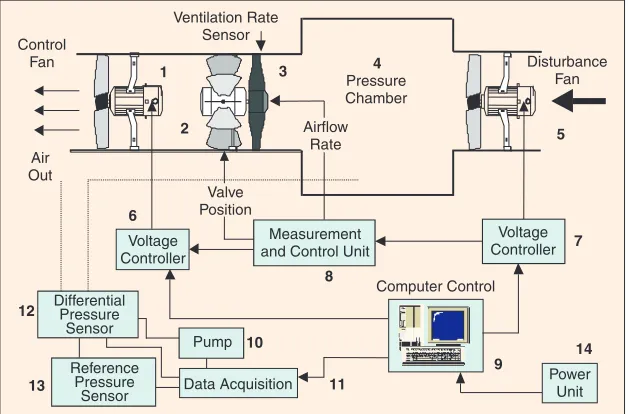
of the fans used in the forced ventilation systems. Fig. 6, for

example, is a diagram of the fan test installation at Leuven.

The model for this system is identified by the SRIV algorithm

as a first-order discrete time TF, and this model has been used

as the basis for PIP and GPC system design. This study

con-firms that the model-based control algorithms offer better

performance than the conventional PID controller in terms of

both the regulation of ventilation rate and the reduction of

energy consumption. In particular, for a 450-mm axial fan, the

normalized mean square errors are as follows: PIP = 1, GPC =

1.64, PID = 5.59. These results were obtained for an airflow

rate of 3000 m

3

/h with realistic wind disturbances, but, in

or-der to evaluate their practical robustness, all three

control-lers were optimized for an airflow rate set point in the

neighborhood of 1500 m

3

/h, without wind.

Environmental Forecasting

Previous publications from Lancaster illustrate how the

modeling and forecasting procedures outlined above have

been applied to environmental and other time series (e.g.,

[13] and the references therein). Here, we will consider the

results obtained in the case of two practically important

en-2

0

−2

−4

−6

−8

−1 0

0

0 100

100 200

200 300

300 400

400 500

500 600

600 700

700 800

800

T

emper

ature [

C]

°

Outlet Temperature Response and Residuals

[image:9.612.61.335.64.259.2]

Time [Tens of Seconds]

Figure 5.

Comparison of the model estimated temperature and the

(10)

vironmental examples: first, the famous

series of monthly atmospheric CO

2

mea-surements at Mauna Loa in Hawaii, as

shown in Fig. 7, which did much to

pro-mote the current debate on global

warm-ing; and second, the hourly rainfall and

river flow series from the River Ribble

Catchment in northwest England, as

shown in Fig. 8.

Adaptive Forecasting,

Backcasting,

and Interpolation of the

Mauna Loa CO

2

Series

It is clear from Fig. 7 that the variations in

atmospheric CO

2

at Mauna Loa are

domi-nated by a long-term, upward trend and

an-nual periodicity. As a result, the identified

UC model takes the form

y

t

= +

T

t

C

t

+

e

t

(5)

where

T

t

a

a t

d

t

C

t

a

j t

t

b

j

j j t

=

+

=

+

=

∑

0 1 2

2

1 2

and

,

cos(

ω

)

,

(sin

ω

j

t

)

(6)

and

y

_t

denotes theCO

2

. As shown, the trend

T

t

is identified as

a polynomial in time

t

, with unknown but

constant

parame-ters, combined with a residual signal

d

_t

that models the

me-dium-term, stochastic deviations about this polynomial

trend. The annual seasonality is modeled by the periodic

component

C

_t

: this is of a standard trigonometric (Fourier)

form but with stochastically time-varying parameters (TVPs)

a

_{j t}_,

,

b

_{j t}_,

,

j

=

1 2. This type of relationship will model any peri-

,

odic behavior defined by the frequencies

ω

j

,

j

=

1 2, and the

,

TVPs allow for the estimation of changes in the amplitude

and phase of these seasonal variations. In the present CO

2

example, the frequency

ω

1

=

2 π

/

12 is the fundamental

fre-quency associated with the 12-month seasonal cycle, and

ω

2

=

2 π

/ is its first harmonic. The spectrum of the data sug-

6 gests that the other harmonics are insignificant and can be

omitted. The TVPs

d

_t

,

a

_{j t}_,

,

b

_{j t}_,

,

j

=

1 2 in this UC model are

,

identified and modeled as simple random walk processes in

an associated set of stochastic state equations (see [13]).

The hyper-parameters (e.g., noise variance ratios) in this

state-space model are estimated by a special form of

optimi-zation in the frequency domain (see [12] and [13]) and the

recursive KF and FIS algorithms are then used for

forecast-ing, backcastforecast-ing, and interpolation of the series.

Typical results are shown in Figs. 9 and 10. For this

analy-sis, the estimation data set consisted of the first 313 samples

(1958(1)-1985(5)) of the 504 data set, but with two years of

these data between 1971(8) and 1973(8) omitted to show

how the algorithms interpolate over such a gap. For

valida-Control Fan

Air Out

6

12

13

10

11 8

9

14 7 5 4

3 1

2

Voltage Controller

Differential Pressure

Sensor

Reference Pressure

Sensor

Pump

Data Acquisition

Measurement and Control Unit Valve

Position

Pressure Chamber Ventilation Rate

Sensor

Disturbance Fan

Voltage Controller

Computer Control

Power Unit Airflow

[image:10.612.239.553.64.271.2]

Rate

Figure 6.

Schematic layout of the test chamber and associated control equipment.

2.5

2

1.5

1

0.5

0 0

0 50

50 100

100 150

150 200

200 250

250 300

300 350

350 400

400 450

450

Flo

w

Rainfall-Flow Data for River Hodder at Hodder Place

6

4

2

0

Rainf

all

Time [h]

Figure 8.

Hourly rainfall (lower panel) and flow (upper panel)

series for the River Hodder at Hodder Place in the River Ribble

Catchment of northwest England.

370

360

350

340

330

320

310

1960 1965 1970 1975 1980 1985 1990 1995 2000

Carbon Dio

xide [ppm]

Date

[image:10.612.313.551.291.473.2] [image:10.612.313.551.500.696.2]

Atmospheric Carbon Dioxide at Mauna Loa, Hawaii, 1958-2000

(11)

tion purposes, true multistep-ahead forecasting is carried

out in the short term (three years ahead) and long term

(14.4 years ahead to 1999(12)), respectively, based only on

the estimation data set, with the model optimized on the

ba-sis of these same limited data (306 samples). The top panel

in Fig. 9 shows the two-year interpolation results, whereas

the lower panel shows the three-year-ahead forecasts. In

both cases, the results are excellent, with very small errors

between the interpolates/forecasts (full lines) and the data

(dashed lines, not used in the analysis). The estimated

stan-dard error bounds (95% confidence intervals) are shown as

dotted lines. Fig. 10 shows the last 5.5 years of the

14.4-year-ahead forecast. Here, the data (again not used in

the estimation or forecasting) are plotted as circular points

and the forecast as a solid line, with the standard error

bounds shown dotted. Given the very long

forecasting interval, these results are quite

remarkable and show how predictable this

important series can be if sufficiently

pow-erful forecasting algorithms are used. As far

as the authors are aware, these are the best

forecasting results produced so far for this

series.

Adaptive Flow Forecasting

in the Ribble Catchment

Once again, the scientific literature

abounds with different models of

rain-fall-flow processes in river catchments.

These vary considerably in complexity

from those based on continuum mechanics

(solved approximately via finite difference

or finite element spatiotemporal

discre-tization methods) [29] through conceptual

models such as TOPMODEL [30] to

hy-brid-metric-conceptual (HMC) grey-box

models such as IHACRES (e.g., [31]), which

are similar in structure and complexity to

the DBM model equivalent [32]. The main

aim of the River Ribble study [33] was

threefold: first, to obtain DBM models

relat-ing rainfall to the river flows measured in

the Ribble catchment; second, to evaluate

the performance of a state-adaptive,

KF-based approach to forecasting, with

the state dynamics defined by these DBM

models; and finally, to compare this

state-adaptive approach with its

predeces-sor at Lancaster, the parameter-adaptive

forecasting system developed for the

Sol-way River Purification Board as a flood

warning system for the town of Dumfries in

Scotland (e.g., [34]). Another, secondary

objective following from the development

of the Lancaster adaptive radar calibration (ARC) system

for the National Rivers Authority/Environment Agency

[35] was to consider how well forecasting performance

using weather radar measured rainfall compared with the

performance using more conventional ground-based

methods.

In the case of a uniform sampling interval of one hour,

SRIV identification and estimation yields the following

dis-crete-time TF model between the gauged rainfall

r

t

and the

measured flow

y

t

for the River Hodder at Hodder Place in the

Ribble catchment during December 1993:

y

b

b z

a z

g r

t

=

t t

+

−

− − −

0 1

1

1 1

2

2 4

1 {

}

ξ

.

₍₇₎

335

330

325

1971 1971.5 1972 1972.5 1973 1973.5 1974 1974.5

Carbon Dio

xide [ppm]

Carbon Dio

xide [ppm]

Interpolation and Forecasting Results

355

350

345

340

1985 1985.5 1986 1986.5 1987 1987.5 1988 1988.5

[image:11.612.60.369.64.253.2]

Date

Figure 9.

Two-year interpolation (upper panel) and three-year-ahead forecasting

(lower panel) results for the Mauna Loa CO

2

series.

380

375

370

365

360

355

350

1995 1995.5 1996 1996.5 1997 1997.5 1998 1998.5 1999 1999.5 2000 Date

Carbon Dio

xide [ppm]

Long-Term 14 Year-Ahead Forecast, 1986-2000 (Last Five Years Shown)

Figure 10.

Long-term, 14.4-year-ahead forecast of the Mauna Loa CO

2

series,

[image:11.612.60.369.287.510.2]

(12)

Here,

g r

{

t−4

}

is a nonlinear function of the rainfall delayed by

four sampling intervals to introduce the pure (advective)

time delay between the occurrence of the rainfall and its

first measured effect on the river flow. The noise level on

flow data is normally quite large, and the noise term

ξ

t

is

in-troduced here to reflect the combined effects of

measure-ment noise, unmeasured disturbances, and imperfections

in the model.

In this case, SDP estimation shows that a rainfall

nonlinearity is present and takes the form

u

t−4

=

g r

{

t−4

}

= ⋅

c f y

{ }

t

⋅

r

t−4

(8)

where

u

t

is termed the “effective rainfall” (or “rainfall

ex-cess”) and

c

is a scale factor chosen conventionally so that

the volume of the effective rainfall is equal to the total

stream flow volume over the estimation period. Equation

(8) shows that the rainfall affects the flow via a

multiplica-tive nonlinearity between

r

t−4

and a nonlinear function of

flow

f y

{ }, where

t

y

t

is acting as a surrogate for the soil

mois-ture, which is difficult to measure [9]. The estimated

nonlin-ear function shows that the SDP is small for low flows (low

soil moisture) and increases, but with diminishing slope, for

high flows. Consequently, the effective rainfall is lower than

the actual rainfall for low soil moisture, since it tends to be

absorbed by the dry soil under these conditions. At high

flow (high soil moisture), however, the rainfall is much more

effective in inducing flow variations.

Based on this SDP identification analysis and subsequent

parametric estimation, the rainfall-flow nonlinearity is

parametrized using a power law

f y

{ }

t

=

y

t

θ

_{to approximate}

f y

{ }. The SRIV estimates of the associated parameters, as

t

well as the TF parameters, are shown in Table 1. This also

in-cludes some parameters that are derived from

decomposi-tion of the TF model into the following parallel connecdecomposi-tion of

two first-order processes (e.g., [9]):

b

b z

a z

z

0 1

1

1 1

2 2

1

1 1

2

2 1

1

1 +

+

=

+

−

− − − −

β

α

β

α

(9)

where

α

i

and

β

i

,

i

=

1 2 are, respectively, the eigenvalues of

,

the TF denominator and the associated residues in the

par-tial fraction expansion of the TF. The latter define the

weighting or “partitioning” associated with this

decomposi-tion. It is clear from (8) and (9) that the effective rainfall

u

t−4

can be partitioned into two parallel pathways resulting in

two component flows that, when added together, yield the

total measured river flow. In effect, therefore, the

decompo-sition provides estimates of two “unobserved” (“latent” or

“hidden”) flow states and their associated rainfall-flow

dy-namics.

The estimates in Table 1(b) reveal that the two pathways

have very different dynamics. The “quick-flow” pathway has

a total travel time (

T

i

+ δ

) of 7.5 hr, whereas the “slow-flow”

pathway has a total travel time of 77 hr. The associated

par-tition percentages of 60% and 40%, respectively, suggest

that more of the effective rainfall affects the quick-flow

path-way than the slow-flow pathpath-way. Note, however, that if the

uncertainty in the parameter estimates is taken into

ac-count using MCS analysis (see previous discussion and [8]),

then some of the derived parameters in Table 1 have wide

confidence intervals and non-Gaussian distributions. In

par-ticular, and not surprisingly, the slow-flow dynamics are

much more poorly defined than the quick-flow dynamics.

As we have stressed, an important aspect of DBM

model-ing is the physical interpretation of the model. Given the

de-rived parameters in Table 1, the most obvious physical

interpretation of the model (9) is that the effective rainfall

af-fects the river flow nonlinearly via two main pathways. First,

the initial rapid rise in the hydrograph, following an

instanta-neous rise in effective rainfall, derives from the quick-flow

pathway, probably as the aggregate result of the many

sur-face processes active in the catchment. The subsequent long

tail in the recession of the hydrograph is associated mainly

with the slow-flow component, probably as the result of

wa-ter displacement within the groundwawa-ter system.

For flow forecasting purposes, the complete catchment

model for the River Ribble is formulated in terms of

rain-fall-flow models such as (7), together with flow-flow TF

mod-els that route the flow down the river system. All of these TF

models are then combined into a set of stochastic state

equations with a state vector

x

t

. In the case of the

rain-fall-flow models, such as (7), the associated state variables

are defined as the latent states defined by decompositions

such as (9), and the rainfall inputs are the effective rainfall

series, such as

u

_t

. The estimate

x

$

t

of the state vector

x

t

and,

from this, the recursive estimate

y

$

t

of the river flow

y

t

can

Table 1. (a) Model parameter estimates

(to three decimal places).

Parameter Estimates

$

.

( .

);

$

.

( .

)

a

1

= −

1 739 0 015

a

2

=

0 743 0 014

$

_.

_{( .}

_);

$

_.

_{( .}

₎

b

₀

=

0153 0 006

b

₁

= −

0149 0 005

$

.

;

$

.

;

$

.

;

$

.

α

1

=

0 986

α

2

=

0 753

β

1

=

0 006

β

2

=

0147

$

.

;

$

.

( .

)

c

=

0 847

ϑ

=

0160 0 0001

(b) Derived physically meaningful parameters for (9).

Physically

Meaningful Derived

Parameters

Slow Flow

Quick Flow

SSG,

G

i

0.40

0.60 Residence time,

T

_i

73 hr

3.5 hr

Advective delay,

δ

4 hr

[image:12.612.311.551.65.325.2]

(13)

then be obtained from the associated KF algorithm (see

[11], [33], and [36]), whose stochastic hyper-parameters

(variance ratios) are estimated by maximum likelihood

opti-mization based on prediction error decomposition [37]. The

resulting four-step-ahead forecasting results are obtained

from the prediction step in the KF update equations and are

shown graphically in Fig. 11.

The forecasting performance shown in Fig. 11 can be

im-proved a little if the noise

ξ

t

in (7) is modeled as an AR

pro-cess and introduced into the state-space description (thus

increasing its dimension to include the additional

stochas-tic states). Even without this improvement, however, the

performance is good, and this is reflected in the statistical

properties of the forecast errors, which have a mean value

near zero (0.0032 mm

⋅

hr

-1

) and a standard deviation

σ

e4

=

0132

.

mm

⋅

hr

-1

. The coefficient of determination based

on the variance of the four-step-ahead prediction errors is

R

₄2

0 871

=

.

, compared with

R

₄2

0 484

=

.

for the naïve

(persis-tence) forecast, where the predicted four-hour-ahead flow is

equal to current flow.

Conclusions

This article has briefly reviewed the main aspects of the

ge-neric DBM approach to modeling stochastic dynamic

sys-tems and shown how it is being applied to the analysis,

forecasting, and control of environmental and agricultural

systems. The advantages of this inductive approach to

mod-eling lie in its wide range of applicability. It can be used to

model linear, nonstationary, and nonlinear stochastic

sys-tems, and its exploitation of recursive estimation means

that the modeling results are useful for both online and

offline applications. To demonstrate the practical utility of

the various methodological tools that underpin the DBM

ap-proach, the article also outlined several typical,

practical examples in the area of environmental and

agricultural systems analysis, where DBM models

have formed the basis for simulation model

reduc-tion, control system design, and forecasting.

How-ever, the same methods have been used in many

other applications in diverse areas of science and

social science. Recent applications include:

• Engineering

: the delta operator modeling and

autostabilization of the Harrier VSTOL aircraft

in its most difficult transitional mode between

hovering and normal flight [7], [16], the

model-ing and control of interurban traffic systems

[38], and both model reduction and control of

an industrial gasifier system [39].

• Ecology

: the modeling of limit cycling

behav-ior in blowfly population dynamics [7], [14].

• Biology

: DBM modeling has revealed new

as-pects of the dynamics associated with

stomatal behavior in plants [40]; the chaotic

electrical activity in the axon of a squid has

also been modeled [41], [42].

• Business Data Analysis and Forecasting

: UC modeling

and forecasting of microeconomic and business data

for the credit card company Barclaycard, U.K. [43]

• Macroeconomics

: where DBM modeling yields some

thought-provoking, and rather topical, insights into

the relationship between government spending,

pri-vate capital expenditure, and unemployment in the

United States between 1948 and 1998 [44].

Acknowledgments

The authors are grateful to the United Kingdom

Biotechnol-ogy and Biological Sciences Research Council for its

sup-port, through Research Grants 89/E06813 and 89/MMI09731,

together with the Ph.D. studentship 98/B1/E/04226. The

au-thors would also like to thank all the past and present

mem-bers of the Environmental Systems and Control Group in

CRES at Lancaster University who have contributed to the

research described in this article, as well as Prof. Daniel

Berckmans and his staff in the Laboratory for Agricultural

Buildings Research at the Katholieke Universiteit Leuven,

Belgium.

References

[1] K.J. Beven, “Phrophecy, reality and uncertainty in distributed hydrologi-cal modelling,”Adv. Water Resources, vol. 16, pp. 41-51, 1993.

[2] K. Keesman and G. Van Straten, “Set membership approach to identifica-tion and predicidentifica-tion of lake eutrophicaidentifica-tion,”Water Resources Research, vol. 26, pp. 2643-2652, 1990.

[3] S. Parkinson and P.C. Young, “Uncertainty and sensitivity in global carbon cycle modelling,”Climate Res., vol. 9, pp. 157-174, 1998.

[4] K. Hasselmann, “Climate-change research after Kyoto,”Nature, vol. 390,

pp. 225-226, 1997.

[5] I. Seginer, “Some artificial neural network applications to greenhouse en-vironmental control,”Comput. Electron. Agriculture, vol. 18, pp. 167-186, 1997.

2.5 2 1.5 1 0.5 0

State-Adaptive Four-Step Ahead Forecasting: River Hodder at Hodder Place

0 50 100 150 200 250 300 350 400 450 Time [h]

Flo

[image:13.612.61.335.63.285.2]

w [mm/h]