Lancaster University Management School
Working Paper
2004/037
Re-employment Hazard of Displaced German Workers:
Evidence from the GSOEP
Haile, Getinet Astatike
The Department of Economics Lancaster University Management School
Lancaster LA1 4YX UK
©Haile, Getinet Astatike
All rights reserved. Short sections of text, not to exceed two paragraphs, may be quoted without explicit permission,
provided that full acknowledgement is given.
The LUMS Working Papers series can be accessed at http://www.lums.co.uk/publications/
Re-employment Hazard of Displaced German Workers:
Evidence from the GSOEP
Getinet Astatike Haile
Department of Economics
Lancaster University Management School Lancaster LA1 4YX.
Re-employment Hazard of Displaced German Workers:
Evidence from the GSOEP
Abstract
This study investigates the re-employment hazard of displaced German workers. It uses data from the first fourteen sweeps of the German Socio-Economic Panel (GSOEP) survey for the purpose. The paper employs both parametric and non-parametric discrete-time models to study the re-employment hazard. Alternative mixing distributions have also been used to account for unobserved heterogeneity. Results based on single risk models show that the average hazard rate of exit via re-employment declines with the duration of time in unemployment. Accounting for unobserved heterogeneity does make a difference, but the crux of the results in terms of duration dependence remains largely unchanged. In terms of covariate effects, those at the lower end of the skills ladder, those who had been working in the manufacturing industry and those with previous experience of inactivity are found to have lower hazard of exit via re-employment. That those at the lower end of the skills ladder and those with previous experience of inactivity have difficulty getting re-employed calls for appropriate intervention to ameliorate the lot of the ‘disadvantaged’.
Theme: Microeconomics of unemployment
Key words: Unemployment duration, job displacement, Germany
1. Introduction
The problem of unemployment has been featuring top of the European labour market
literature for sometime now. Two of the most prominent discourses in this regard relate
to the persistence of high unemployment in recent decades (Nickell, 2003; Heckman,
2002; Blanchard and Wolfers, 2000) and the contrast between the levels of
unemployment in the US and the European labour markets (Nickell, 1997; 2003;
Blanchard and Portugal, 2001; Heckman, 2002; Siebert, 1997; Blank, 1994). Both these
aspects of the unemployment situation in Europe have been attributed to adverse shocks,
adverse institutions and the interactions of the two. What has become common
explanation more recently, particularly in relation to European labour markets, has to do
with the role of institutions and how they respond to adverse shocks. The consensus in
this regard is that labour market rigidities1 have, at least in some of these labour markets,
led to the rise in the level of unemployment by affecting the equilibrium level of
unemployment as well as deviations of actual unemployment from its equilibrium level.
The system of unemployment benefit and the type of employment protection scheme in
place are, in particular, regarded to be important factors behind the high level of
unemployment in these countries.
Labour market rigidities are likely to influence the equilibrium level of unemployment in
several ways. They can affect the way in which unemployed individuals can be matched
1 Labour market rigidities refer to a number of labour market characteristics including the presence of
to available job vacancies. They also tend to raise the wage rate even when there is
excess supply of labour. By lowering the search intensity of the unemployed, for
example, the system of unemployment benefit in place - its level and the duration it lasts
- reduces the readiness of the unemployed to fill available vacancies. Employment
protection laws, on the other hand, are likely to make firms more cautious regarding
filling available vacancies and, therefore, may lower the speed with which the
unemployed may take up jobs. Because such laws are primarily meant to protect jobs,
however, they also have the tendency to curtail involuntary separations and, therefore,
lower inflows into unemployment. As such, therefore, the effect of employment
protection schemes on the equilibrium level of unemployment may not be clear-cut.
Nevertheless, at least in the countries that have been experiencing high levels of
unemployment, one typical observation has to do with the prevalence of long-term
unemployment. This means that the system of benefits in place and the type of
employment schemes in place have made the labour markets of these countries rather
stagnant.
The German labour market has been regarded as a typical case of the European labour
markets exhibiting most signs of rigidity. The evidence in most recent studies that look
into the nature of unemployment in Europe supports this claim. Nickell (1997; 2003),
Bender et al (2002), Heckman (2002) and Blanchard and Wolfers (2000) are some of the
most recent studies that look into labour market rigidities in terms of high employment
protection, generous benefit schemes, strong presence of labour unions, wage-setting
to a substantial increase in the share of long-term unemployed people who have been
unemployed for over 12 months (Steiner, 2001; Nickell, 2003).
Long-term unemployment has particularly adverse effects to individuals experiencing it
and society at large in many respects. To begin with, the long-term unemployed are likely
to be discouraged to carry on searching for jobs. Because of the likely scaring effect of
long-term unemployment, firms may not also be willing to take on such workers. It is
also possible that such workers lose, at least in part, whatever skill they have if they stay
unemployed for long. The combined effect of these will be to make unemployment even
more persistent and possibly bring about poverty and social exclusion to the particular
segment of the labour force that experiences such long-term unemployment
(Arulampalam et al, 2001).
The types of workers that are most likely to suffer from the adverse effects of long-term
unemployment are displaced workers who separate from their jobs involuntarily. The
presence of high long-term unemployment due to labour market rigidities means that
there are barriers to re-entry into the job market, and such difficulty of re-entry may
particularly be relevant to displaced workers. It may also be the case that some segment
of the displaced may fare particularly worse. Displaced workers that are at the lower level
of the skill/qualification ladder may bear the brunt of the unemployment problem as a
result of labour market rigidities. In the context of the German labour market, such
workers form the bulk of displaced workers (Haile, 2002). The combination of
deadly for these workers, as firms may not be willing to take the risk of hiring them
(Blanchard, 1998).
In this study I investigate how displaced workers fare in terms of the duration of time that
they spend unemployed. There are very few studies2 that investigate the duration of
unemployment in Germany (Hunt, 1995; 1997; Steiner, 1994; 2001) and even fewer that
focus on the unemployment duration of displaced workers in particular (Couch, 2001;
Bender et al, 2002). It is therefore evident that not much is known regarding the duration
of unemployment that unemployed workers in general experience. Most importantly,
there is a huge gap in our knowledge pertaining to the duration of unemployment that
displaced workers experience in Germany.
What is equally important is that there is lack of consensus regarding whether the outflow
rate from unemployment declines as the duration of unemployment lengthens. Broadly
speaking, the evidence on negative duration dependence in Europe is mixed (Machin and
Manning, 1999). Moreover, results on negative duration dependence seem to be sensitive
to the way unobserved heterogeneity is accounted for. Taking these into account, this
study attempts to fill the gap in the literature by studying the duration of displacement
unemployment in Germany.
This study has six parts and has the following structure. In section 2 a review of the
literature on the duration of unemployment will be given focusing mainly on the
2 This is excluding studies that are written in German. Steiner (2001) and Hunt (1995) cite some of the
unemployment duration literature in the context of the German labour market. Section 3
is devoted to the description of the data and sample used in the empirical exercise carried
out in this study. Section 4 gives an account of the econometric specifications and
methods of estimation used for the purpose of studying the duration of displacement
unemployment. Section 5 discusses the estimation results obtained and the final section
concludes the paper.
2. Literature Review
As stated earlier, there are few empirical studies that look into the duration of
unemployment in Germany in general and that of the duration of displacement
unemployment in particular.3 Bender et al (2002) is one of the most recent studies that
look into the duration of non-employment in Germany. Using the administrative social
security data file (IAB) and focusing on separations due to plant closure and other types
of reasons, they analyse the duration of time that displaced workers, those that left job
due to plant closure, and other separators, such as those that were dismissed for cause,
spend in non-employment. They find that displaced workers leave non-employment at a
faster rate than workers who separated for other reasons. This finding is in line with
previous findings (such as Gibbons and Katz, 1991) and is partly the result of the way in
which they define displaced workers. As is generally the case, identifying displaced
workers using administrative data, which relies on whether or not plants have been
3 This might have to do with the fact that displaced workers in Germany do not experience a spell of
closed, is likely to lead to selectivity problem. This definition ignores those workers that
get displaced from declining but still operating plants. Although Bender et al (2002) go
some distance by way of explaining the duration of non-employment that displaced
workers experience, their study is different from this study in a number of ways. First, it
looks at the duration of non-employment as opposed to the duration of unemployment,
which this study is primarily about. Secondly, the way displaced workers have been
identified is likely to suffer from the problem of selectivity bias. Finally, their study does
not address the issue of unobserved heterogeneity, which has been found to play an
important role in explaining the duration of unemployment that displaced and other
unemployed workers experience. Heckman and Singer (1984) and Keifer (1988), among
others, have shown that not accounting for unobserved heterogeneity gives rise to
(downward) biased estimates of duration dependence.
Using the first twelve waves of the German Socio-Economic Panel (GSOEP) data,
Steiner (1994; 2001) investigates whether or not there is unemployment persistence in the
West German labour market. Steiner states that the persistence of high unemployment
has been a serious problem in Germany for many years and argues that the rise in the
unemployment rate has mainly been due to substantial increase in the share of the
long-term unemployed - those who have already been unemployed for at least one year. Using
discrete-time approach with flexible baseline hazard specified as random-effects logit and
accounting for unobserved heterogeneity, Steiner tests whether or not unemployment
persistence in the West German labour market can be explained by negative duration
unemployment are due to unobserved heterogeneity. He finds that once unobserved
heterogeneity is accounted for, negative duration dependence in the employment hazard
rate disappears. In fact, Steiner finds the unobserved heterogeneity controlled hazard rate
for men to be positive.
Steiner (2001)’s study differs from this study for a number of reasons. First, the focus of
his study is on all unemployment spells as opposed to displacement unemployment
spells, which are the prime focus of this study. Secondly, the discrete-time logit
specification used for the hazard of exit from unemployment represents a possible
drawback of his study. Allison (1982) and Vermunt (1996) argue that this specification is
sensitive to the choice of the length of the time intervals, and also necessitates that these
intervals be of equal length. This is because the length of the time interval influences the
probability that an event will occur in a particular interval and it, therefore, influences the
hazard that the event of interest takes place in the interval. The complementary log-log
specification is more appropriate in this context particularly when there are no
time-covariate interactions and with proportional hazard specification. As will be discussed in
Section 4 below, the complementary log-log specification has been used in this study and
it is likely to give rise to better results. Third, unlike Steiner (2001), alternative
specifications will be used in this study by way of accounting for unobserved
heterogeneity. This is likely to give better results in terms of duration dependence and the
Couch (2001) investigates the duration of unemployment that displaced workers
experience using the GSOEP data over the period 1988 – 1996. He estimates the annual
months of unemployment that displaced workers experience using Tobit regression.
Accordingly, the estimated number of months that displaced workers experience in the
year of displacement range from .31 to .48 moths while no significant effect is found in
the years preceding the year of displacement. The approach used in this study is vitally
different from the one used by Couch. In this study, the hazard specification is used to
assess the cost of job displacement in terms of the duration of unemployment displaced
workers experience. As such, therefore, Couch’s findings cannot be compared directly to
findings of this study.
Hunt (1995) uses the GSOEP data over the period 1983 – 1988 to analyse the effect of
unemployment compensation on unemployment duration in Germany. Using the Cox
partial likelihood proportional hazards model, Hunt estimates competing risks of
transitions to employment and inactivity for both men and women. The results from this
study indicate that changes in the law which took the form of increasing the potential
duration of unemployment insurance was found to be an important factor explaining
differences in the patterns of exits to employment and inactivity for men and women in
Germany and also why German unemployment spells are so much longer than American
spells. Hunt (1995) focuses on overall unemployment spells and the effect of the policy
change on the unemployment spells. As such, Hunt’s study differs from this study, which
focuses on displacement unemployment. Methodologically, Hunt (1995) uses the Cox
continuous-time event history data (Vermunt, 1996). As will be detailed in Section 4 of this study,
more appropriate methodology is used in this study to model the duration of
unemployment for displacement and overall unemployment spells in Germany.
3. The Data and Sample
The data used in this study come from the German Socio-Economic Panel (GSOEP). The
first fourteen waves of the GSOEP data covering the period 1984 to 1997 have been sued.
In addition to the contemporaneous information collected at the interview date of each
wave of the GSOEP, recall information is collected on labour market activities of
respondents in each month in the preceding calendar year. Combining the
contemporaneous/yearly information on labour market status of respondents with the
recall/monthly information on labour market activity, a sequence of monthly labour
market status has been constructed for each subject included in the duration analysis
made in this study.
This data construction process has two main parts. The first part involves carefully
selecting individuals on the basis of some sample selection criteria that were applied to
the yearly information of the GSOEP. Accordingly, individuals of working age (16 – 64)
from samples A and B of the GSOEP4 that have been interviewed successfully at each
wave over the period considered in this study have been chosen first. Then selection was
4 Samples A and B are the initial samples of the GSOEP representing West Germans and foreigners
made on the basis of some criteria. The first such criterion involves excluding individuals
that reported to have worked in activities/industries such as agriculture that are regarded
to represent heavy subsidisation over the years in a way that does not conform to the
normal operation of the labour market. The second criterion involves excluding those
individuals that were in self-employment. Individuals in this category too are not
generally considered to make up an ideal sample for the purpose of studying the costs of
job displacement stemming from the workings of the labour market. Individuals with
gaps in observation are the next group of people that have to be excluded from the sample
used for the duration analysis. After imposing these restrictions a final sample has been
obtained by matching the different person and household level data files of the GSOEP.5
The yearly panel constructed in this way consists of a total of 8,055 individuals that have
been covered by the GSOEP in any year over the study period. Of this total, 2,824 have
appeared in every wave over the period considered in this study.
The second part of the data construction process to get the sample of displacement
unemployment spells used in this study involved merging the yearly panel briefly
described earlier with the recall information from the calendar data files. This gave rise to
an initial panel consisting of 6,081 individuals and 660,288 person-month observations.
Two restrictions have been imposed to this initial sample. First, those individuals with
gaps in person-month information have been removed from the sample. Second, those
individuals with severe inconsistencies between their contemporaneous and recall labour
market status were also eliminated from the sample. These two restrictions and the
elimination of left-censored non-employment labour market status gave rise to the second
panel consisting of 4,913 individuals and 508,565 person-month observations.
The next stage of construction of the sample of GSOEP unemployment spells involved
copying the contemporaneous personal, household, regional and labour market
information to each and every person-month observation using a series of rules.6 Keeping
only unemployment spells that were preceded by a spell of employment and with valid
contemporaneous information on relevant covariates gave rise to the final sample of 1022
individuals and 16,620 person-month observations. Of these, 949 individuals with 13,974
person-month observations of unemployment spells make up the sample of displacement
unemployment spells. The remaining 191 individuals with 2,646 person-month
observations of unemployment spells represent non-displacement unemployment spells.
The total number of people in the two samples of unemployment indicates that there are
some people who experienced unemployment as a result of both job displacement and
‘other’ reasons during the sample period.
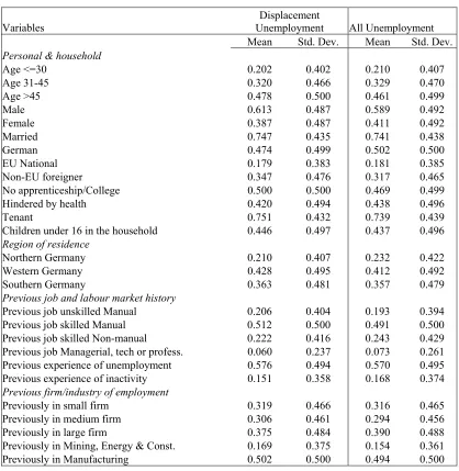
Table A1 in the appendix gives a summary of the variables used in the duration analysis
made in this study. As can be seen from the table, most of the unemployment spells are
the result of job displacement. Most of those that experience displacement unemployment
are men, married and over 45 years of age. Most of the displaced unemployed are also
6 The series of rules applied for the purpose of copying contemporaneous information to each person-month
Germans residing in rented houses and with no/incomplete apprenticeship and/or
higher-level qualification. Most of the displaced unemployed also have some health condition
that hinders their day-to-day activity/work. Most also come from Western Germany
which includes the regions North Rhine Westphalia; Hesse and Rhineland-Palatinate; as
well as Saarland. Most of the displaced unemployed had skilled manual job and were
working in large firms in the manufacturing industry in their previous employment.
Moreover, well over 50 per cent of the displaced unemployed had some prior experience
of unemployment.
4. Model specifications and methods of estimation
That the duration variable of interest to this study is measured to the nearest month means
that the appropriate approach to modelling the duration of unemployment is the
discrete-time hazard model. The estimation of discrete-discrete-time duration models requires expanded or
person-period data set organised in such a way that there will be as many data rows for
each individual in the sample as there are time intervals over which the individual in
question is at risk of experiencing the event of interest - re-employment here. The
creation of such expanded person-period (person-month) data is a crucial part of the
discrete time hazard modelling exercise as it ensures that the likelihood contribution of
each individual is properly accounted for (Jenkins, 1997; 2003).
Following Cox (1972), Prentice and Gloecker (1978) and Meyer (1990), the discrete time
proportional hazards model. Accordingly, the hazard of re-employment in the jth month,
h(tj), for individual i with a vector of covariates, x, having spent t months in
unemployment and given that re-employment has not occurred before tj-1 can be given by
)]) ( ) ( exp[ exp( 1 ) |
( j xi j xiβ
ij t t
h = − − γ + ′ (1)
Rearranging the discrete-time hazard given in equation (1) gives what is known as the
complementary log-log transformation of the conditional probability of exiting the state
of unemployment at time tj as
) ( ))) | ( 1 ln(
ln(− −hij tj xi =x′iβ+γj t (2)
Given this complementary log-log transformation, the parameter is interpreted as the
effect of covariates in x on the hazard rate of re-employment in interval j, assuming the
hazard rate to be constant over the jth interval. The log-likelihood function for the sample
of individuals used in this study can be given by
β
∑∑
∑∑
= = = = − + − = n i t j ij n i t j ij ijit h h
h y L 1 1 1 1 ) 1 log( 1 log log
∑∑
[
(
)
(
)
]
(3)= = − − + = n i t
j it ij it ij
t h y t h y 1 1 | ( 1 log 1 ) | (
As stated earlier, it is well established in the duration literature that not accounting for
unobserved heterogeneity might lead to biased estimates of the baseline hazard as well as
the covariate effects on the hazard of exit from the sate of unemployment (Heckman and
Singer, 1984; Lancaster, 1990). Taking this into account, an attempt has been made in
this study to control for unobserved heterogeneity. The standard practice in the literature
is to introduce a positive-valued random variable (mixture), v, into the hazard
specification. In the context of the discrete-time approach, the augmented hazard
function, which incorporates a multiplicative mixture term, is given by
i i j i i j
ij t v h t v
h ( ,x | )= 0( )exp(x′β ) (4)
The complementary log-log version of equation (4) is then given by
)) ) ( exp( exp( 1 ) | ,
( j i i i j i
ij t v t u
h x = − − x′β+γ + (5)
where, as before, ui =logvi and
∫
− = j t j t du u h t 1 0
j( ) ( ) .
γ
The discrete-time likelihood function that incorporates the unobserved heterogeneity term
is obtained by summing the discrete-time likelihood functions of each individual i that
can be given by
i i u t j ij y i i j ij y i i j
i h t u h t u g u du
L ( , , ) ( , | ) [1 ( , | )] ( )
1 1
∫ ∏
+∞ ∞ − = − −= x x
σ γ
where and ( , | ) 1 exp[ exp( ' ( ) )]
i j
i i
j t v t u
h x = − − x β+γ + σ is the vector of unknown
parameters in The unobserved heterogeneity term is assumed to be independent of
observed covariates, x , and the random duration variable, T, and have density It
is possible to solve the integral in expression (6) to obtain the appropriate density for the
monthly duration information that is organised in a sequential binary response format
(Stewart, 1996; Andrews, et al. 2002; Dolton and van der Klaauw, 1995; Wooldridge,
2002).
). (u gu
i gv(v).
Solving the mixing distribution specified in equation (6) necessitates making specific
distributional assumption for the density of the mixing distribution. The distributional
assumption may either be parametric or non-parametric. The parametric approach
specifies a particular functional form for the mixing distribution.7 The non-parametric
approach, on the other hand, uses the mass point approach pioneered by Heckman and
Singer (1984), where the mixing distribution is approximated by a finite discrete
distribution of unrestricted form. In the absence of theoretical justification for using one
or the other approach for the purpose of approximating the mixing distribution, it may be
reasonable to try and employ both approaches. The parametric distribution assumed in
this study in order to approximate the mixing distribution is the Gaussian distribution8
7 There are several candidates for the parametric mixing density distribution. However, the choice of a
particular parametric distribution is generally harder to justify than the choice of functional form for the baseline hazard. This is due to the fact that economic theory may suggest a particular functional form for the baseline hazard but not for the mixing distribution (Van den Berg, 2001).
8 An attempt has been made to estimate Gamma mixture model using PGHAMZ. However, the model fails
while the non-parametric approach follows the mass pint technique of Heckman-Singer.
The Gaussian distribution does not yield a closed form solution. However, its use is
justified if one views the heterogeneity term as being a combination of a ‘vast number of
minor characteristics of the unemployed individual that are not observed by the
investigator’ (Stewart, 1996). In the case of the non-parametric technique, the unknown
distribution of the unobserved heterogeneity is approximated using discrete distribution.
The mass points and the associated probabilities of the discrete distribution are estimated
jointly with other parameters of the model.9
The second issue of importance in relation to estimating alternative models has to do with
the way the baseline hazard is specified. The baseline hazard can be specified either
parametrically or semi-parametrically. In the case of parametric specification for the
baseline hazard, a particular functional form is assumed for the same. Although there is
no strong theoretical justification for it, the Weibull is the commonly used parametric
specification for the baseline hazard in the unemployment duration literature. Taking this
into account, the first model estimated assumes Weibull for the baseline hazard and this
variant is estimated with and without consideration for unobserved heterogeneity.
Semi-parametrically, the baseline hazard is estimated together with other parameters of the
model. Imposing a particular functional form for the baseline hazard may lead to the
problem of misspecification. A way round this possible problem is to estimate the
analytically tractable and gives closed form solution for the relevant likelihood function (Lancaster 1990; Meyer 1990; Stewart 1996; Van den Berg 2000).
9 See Stewart (1996) and Andrews et al (2001) for the likelihood functions of the Gaussian. For the
baseline hazard semi-parametrically in line with Han and Hausman (1990), Meyer (1990,
1995) and others. Because there are no events in some months, the monthly time intervals
in this study had to be regrouped into just seven time periods for the sake of
identification. The piece-wise constant baseline hazard specification is therefore the
preferred non-parametric specification for the baseline hazard estimated in this study.
5. Estimation Results and Discussion
In this section discussion of results from the estimation exercise will be made. The first
set of results in this study is that which is based on the Weibull specification for the
baseline hazard while the second set of results is from the piece-wise constant baseline
hazard specification. Results from the Weibull model are given in Table 1. Results from
the piece-wise constant model are given in Table 2 and Table 3. In what follows
discussion of these results will be made.
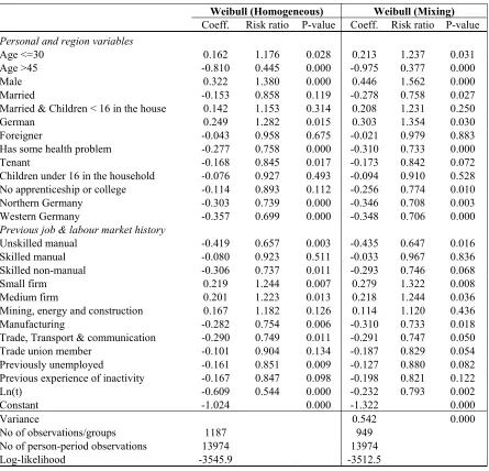
5.1. Results from Weibull model
The first set of estimation results is from the most commonly used Weibull specification
for the baseline hazard. The Weibull model imposes a particular monotonic shape for the
baseline hazard. Both homogeneous and mixing discrete-time Weibull models have been
estimated. The mixing model estimated assumes that the heterogeneity term is distributed
normally. As can be seen from the estimation results in Tables 1, the estimated
coefficients in the mixing models are slightly large in absolute value terms. Likelihood
importance of accounting for unobserved heterogeneity. The coefficient on ln(t) in the
context of discrete-time duration models is an estimate of the parameter describing the
baseline hazard. The estimated coefficient shows that the baseline hazard declines with
time, indicating negative duration dependence. In other words, the longer that an
unemployed individual stays unemployed, the more difficult it will be (for the individual)
to leave the state of unemployment. Accounting for unobserved heterogeneity does make
a difference in the sense that the parameter describing the baseline hazard is less negative
in the mixing Weibull model than its homogenous counterpart. This indicates that
although accounting for unobserved heterogeneity does not eliminate negative duration
dependence completely as in Steiner (2001), it is quite important in explaining whether or
not there is negative duration dependence in the re-employment pattern of displaced
workers.
Referring to the estimated coefficients of the covariates included in the models reveal
how they affect the hazard of re-employment. Accordingly, older displaced workers are
found to have a lower hazard of re-employment compared with their younger
counterparts. In particular, those displaced unemployed that are over 45 years of age have
a 62 percent less hazard of exit to re-employment compared with those that are between
30 and 45 years of age. On the other hand, those displaced unemployed that are less than
30 years of age have a higher hazard of exit to re-employment compared with their older
counterparts who are between 30 and 45 years of age. These findings are in line with
expectation. Older people are more likely to receive fewer job offers given that they are a
of working for longer periods. Young workers are also more capable to learn new skills
that best suit changing demand situations compared with their older counterparts who
may be relatively less suited when it comes to learning new tricks. Also older workers
may decline to accept more jobs than their younger counterparts for various reasons.
Mobility problem as a result of family and other responsibilities, for example, may force
older people to reject some job offers.
Men who are unemployed due to displacement have a 56 percent higher hazard of
re-employment compared with women. There can be different explanation for this. To start
with, men account for more than 60 per cent of the displaced unemployed as can be seen
from Table A1 in the appendix. That men are dominantly represented in the sample of
displacement unemployment spells should mean that they face a greater risk of exit from
unemployment. Another explanation relates to the type of previous jobs that the displaced
unemployed had. More than 70 per cent of previous jobs left are manual type, mostly
involving men. Assuming re-employment to more or less similar type of employment as
before, it would not be surprising to find that men have a higher hazard of exit to
re-employment. Another explanation that best fits the labour economics literature is, of
course, that which relates to the gender difference in the labour market behaviour of
workers. Men are generally expected to receive more job offers than women do mainly
due to the labour market behaviour of women that is characterised by (or perceived to be)
Those that are married displaced unemployed have a 24 percent less hazard of getting
re-employed compared with their single counterparts. Germans who lost their job as a result
of displacement have a 35 percent higher hazard of getting re-employed compared with
EU nationals residing in Germany. On the other hand, foreigners are found to have a
lower hazard of exiting via re-employment although this effect is found to be statistically
insignificant. This means that non-Germans have a longer unemployment duration
compared with Germans. This is in line with expectation given that Germans are likely to
receive more job offers vis-à-vis their non-German counterparts. It should also be noted
that Germans are dominantly represented in the sample of unemployment spells. Those
displaced unemployed who have some health condition/problem have a 27 percent less
hazard of getting re-employed. Those displaced unemployed that do not have own
dwelling have a 16 percent less hazard of securing re-employment. Such workers are
more likely to have a higher offer acceptance rate, and the lower hazard of getting
re-employed should stem largely from lower arrival rate of job offers.
Type of qualification of the unemployed is found to be an important factor explaining the
hazard of exit from the state of unemployment. Accordingly, those displaced workers
without apprenticeship and/or college level training who experienced a spell of
unemployment following job displacement have a 23 percent less hazard of being
re-employed compared with their counterparts with completed apprenticeship and/or college
level training. This finding is in line with what one would expect. Those with the least
qualification are less likely to receive many job offers and hence are less likely to exit
least qualification are more likely to have lower reservation wage and hence are more
likely to accept offered jobs. The net effect therefore depends on which effect is stronger.
In this case, the result seems to imply that the former effect is stronger.
The estimated results also suggest strong regional variation in the patterns of exit from
unemployment via re-employment for the unemployed. Those displaced unemployed in
Northern and Western Germany have longer duration of unemployment compared with
their counterparts in the south of the country. In particular, those workers in the north and
west of the country have a 29 percent lower hazard rate of re-employment compared with
their counterparts in Southern Germany. The regional variables used here serve as proxy
for local labour market conditions that are usually captured using local unemployment
and vacancy rates. Although the region variables hide lots of variations that may exit
among the 10 regions that the GSOEP samples come from, this result can be interpreted
in terms of the respective unemployment and vacancy rates in the regional groups
considered here.
Previous job and labour market history related covariates are the other most important
factors explaining the hazard of exit from unemployment. Accordingly, those displaced
unemployed individuals who had unskilled manual job have longer durations of
unemployment compared with their counterparts who had managerial, technical or
professional job. In terms of the hazard of exit to re-employment, these workers have a
35 percent lower hazard of re-employment compared with their counterparts. Another
hazard of finding re-employment vis-à-vis those that had been working in large firms.
Focusing on the displaced unemployed, those who had been working in small and
medium size firms have 32 percent and 24 percent higher hazards of re-employment,
respectively, compared with those who had been working in large size firms. This could
be attributed to the strong possibility that those with some experience working for smaller
firms are more mobile given that there are relatively more firms of the smaller/medium
type. Institutional factors such as the presence of labour unions and labour protection
schemes in place may tend to be stronger in large firms, making re-employment in the
same (similar size) firm difficult.
Those who got displaced from the manufacturing as well as the trade, transport and
communication industries have a lower hazard of exit via re-employment. This is likely
to be the result of fewer job offers coming from the manufacturing sector, in particular,
which is generally regarded as a sector in decline. Those who were trade union members
in their previous job are found to have a lower hazard of exit via re-employment.
Specifically, displaced workers who were trade union members have a 17 percent lower
hazard of securing re-employment compared with displaced unemployed workers who
were not trade union members. This might be attributed to a relatively lower offer
acceptance rate that former trade union members may have. Such workers might have
been getting some wage premium in their previous job and could have a higher
reservation wage. Another interesting result is that those who got displaced and had been
with other displaced unemployed individuals with no prior unemployment experience.
Previous experience of inactivity also reduces the hazard of exit from unemployment.
5.2. Results from non-parametric models
As discussed earlier, parametric models such as the Weibull assume a particular shape for
the baseline hazard. Assigning a particular shape for the baseline hazard may prove to be
a major shortcoming in duration analysis. In the context of proportional hazards models,
a number of studies including Meyer (1990); Han and Hausman (1990) and Trussell and
Richard (1985) have shown that assigning a specific parametric density for the baseline
hazard can lead to a more serious problem of misspecification than that caused due to
disregarding unobserved heterogeneity. In the face of such evidence, it is reasonable to
adopt semi-parametric specification for the baseline hazard. Such specification has an
additional advantage in that parameter estimates will be less sensitive to the distributional
assumptions made for unobserved heterogeneity. A likelihood ratio test comparing
differences in likelihood scores between the Weibull and the piece-wise constant models
also suggest significant improvements in fit of the piece-wise constant models. Given
these, the estimation results presented in Tables 2 and 3, which are based on piece-wise
constant specification for the baseline hazard, are the preferred results explaining the
duration of displacement unemployment in Germany.
The first piece-wise constant baseline hazard model estimated is the homogeneous
heterogeneity. Then two mixing proportional hazards models have been estimated. The
mixing proportional hazards models estimated are the Gaussian mixing10 and the
non-parametric Heckman-Singer mixing models.11 Estimating alternative mixing distributions
enable us to assess the sensitivity of estimated parameters across the models and whether
or not unobserved heterogeneity is worth considering.
5.2.1. Baseline hazards
Estimates of piece-wise constant baseline hazards from the homogeneous and the two
mixing distributions are given in Table 2. These results are obtained using the
complementary log-log transformation given in equations (1) above by setting all
covariate values equal to zero.12 The first important result worthy of a note has to do with
the rejection of the null hypothesis of zero unobserved heterogeneity. The likelihood ratio
test of zero unobserved heterogeneity for the mixing distributions is strongly rejected
with a P-value of almost zero. As can be seen from the estimated results in Table 2, the
estimated baseline hazards are strikingly similar for the Gaussian and Non-parametric
distributions, lending support to Meyer (1990)’s suggestion that using a flexible
specification for the baseline hazard removes the sensitivity of estimated parameters to
10 The default number of quadrature points in STATA is 12. The default quadrature points have been used
in this study but checks have been made using quadrature check and the results remain more or less the same.
11 The empirical estimation of the discrete mass point approach made in this study has been carried out
using GLLAMM. GLLAMM is a computationally efficient program that fits a large class of multilevel latent variable models including multilevel generalised linear mixed models (Rabe-Hesketh et al., 2002)
12 As stated earlier, the monthly time period has been regrouped to get only seven time periods The
the type of distribution assumed for unobserved heterogeneity. For the homogeneous
distribution, the baseline hazard estimates are higher than those obtained using the
mixing distributions for the first two time periods. After the second period, however, the
baseline hazard estimates from the homogeneous model are found to be less than those of
the mixing distributions. These patterns are shown in figure 1 below where the plot of the
homogeneous baseline hazard drops faster than those of the mixing distributions.
Although there are some differences in the magnitude of the estimated hazards from the
three models, the general patterns observed are more or less similar. Accounting for
unobserved heterogeneity does reduce the observed (negative) duration dependence. As
such, therefore, these results are in line with the common claim in the literature that
accounting for unobserved heterogeneity reduces negative duration dependence.
Time period
7.0 6.0 5.0 4.0 3.0 2.0 1.0
Hazard
.3
.2
.1
0.0
Homogeneous
Gaussian
[image:28.612.181.437.407.621.2]Heckman-Singer
Baseline hazard estimates for the homogeneous model exhibit more or less continuous
decline in the estimated hazards of exit via re-employment. Results from the mixing
distributions, on the other hand, tell a slightly different but more appealing story. For the
displacement unemployment sample, the hazard estimates form the mixing distributions
increase initially and then decline more or less continuously afterwards. This might
indicate that displaced unemployed workers are likely to find re-employment more
difficult if they fail to secure re-employment in the first three months following
displacement.
5.2.2. Effects of covariates
Results showing the estimated effects of covariates on the hazard of re-employment are
given in Table 3. The effects of covariates on the hazard of exit via re-employment are
more or less similar across the three models estimated, with only marginal differences.
The results from the non-parametric models also show some similarity to the earlier
results from the Weibull model. Comparing the maximum of the log-likelihoods from the
piece-wise constant models shows that the Gaussian model has an edge over the other
two models. As a result, discussion of the covariate effects on the hazard of
re-employment made below relies on the Gaussian model.
Starting with the effect of personal characteristics on the hazard of exit via
re-employment, older displaced workers have a 59 percent lower hazard of re-employment
compared with those that are between 30 and 45 years of age. On the other hand, those
higher hazard of re-employment compared with the reference group of displaced
unemployed individuals between 30 and 45 years of age. Same reasoning as given earlier
in relation to results from the Weibull model can be given here in relation to these results.
Men who are unemployed due to displacement have a 53 percent higher hazard of
re-employment compared with their women counterparts. Those that are married displaced
unemployed have a 21 percent lower hazard of re-employment. Germans have a higher
hazard of re-employment while there is hardly a difference between the re-employment
hazards of foreigners and EU nationals residing in Germany. Displaced unemployed
individuals with some health problem have a longer duration of unemployment compared
with their counterparts with no such problem. Those displaced unemployed that do not
own their own dwelling have a 16 percent lower hazard of re-employment. In terms of
the type of qualification of the unemployed, those displaced unemployed workers without
apprenticeship and/or college level training have longer duration of unemployment
compared with displaced unemployed workers with completed apprenticeship and/or
college level training. In terms of region, those residing in Northern and Western
Germany tend to have longer unemployment duration compared with their counterparts
in the South of the country.
As before, previous job and labour market history related covariates are important
determinants of the re-employment hazard. Accordingly, those displaced unemployed
individuals who had unskilled manual job have longer duration of unemployment with a
managerial, technical or professional job. In comparison, those displaced workers who
were working skilled non-manual job have a 25 percent lower hazard of re-employment.
As in the earlier result, firm size too has been found to have an important role in
explaining the hazard of exit via re-employment. Accordingly, those who had been
working in small and medium size firms have shorter unemployment durations with a 28
percent and 18 percent higher hazard of re-employment compared with their counterparts
who had been working in large firms.
Workers who got displaced from the manufacturing and the trade, transport and
communication industries have longer duration of unemployment with a 25 percent and
23 percent lower hazards of re-employment, respectively, compared with those
previously working in the finance, insurance and services industry. On the other hand,
those who were working in the mining, energy and construction industry have a 13
percent higher hazard of exiting unemployment for job. Those who were trade union
members in their previous job are found to have a lower hazard of exit from
unemployment. Specifically, displaced workers who were trade union members have 14
percent lower hazard of re-employment compared with displaced unemployed workers
who were not trade union members. Another interesting result is that those who got
displaced and had been previously unemployed have 15 percent lower hazard of
re-employment compared with other displaced unemployed individuals with no prior
unemployment experience. On the other hand, those with previous experience of
unemployed individuals who had been out of the labour market at some point in the past
have a 19 percent lower hazard of re-employment.
6. Conclusion
This paper attempted to study the duration of unemployment in Germany as part of the
drive to establish on the costs, in terms of unemployment, that displaced workers
experience. The focus of the study has been on unemployment spells that were initiated
as a result of job displacement as a result. Parametric and non-parametric discrete-time
models have been used to study the duration of displacement unemployment spells. In
addition, alternative mixing distributions have also been employed to account for
unobserved heterogeneity. The results obtained indicate that there is evidence of negative
duration dependence in the hazard of exit via re-employment. Accounting for unobserved
heterogeneity does matter, but the main finding of this study with regards to duration
dependence remains unchanged.
With regards to the effect of covariates on the hazard of re-employment, those displaced
workers who are at the lower end of the skills ladder, those who had been working in the
manufacturing industry and those with previous experience of inactivity are found to
have particularly lower hazard of exit via re-employment. The fact that those at the lower
end of the skills ladder and those with previous experience of inactivity have difficulty
exiting unemployment calls for appropriate intervention to ameliorate the condition of the
References
Allison, P. D. (1982), “Discrete-time methods for the analysis of event histories,”
Sociological Methodology, 13, 61 – 98.
Andrew, M. J., S. Bradley and D. Stott (2001), “The School-To-Work Transition, Skill Preference and Matching,” Working Paper, Lancaster University.
Andrew, M. J., S. Bradley and D. Stott (2002), “Matching the Demand for and Supply of Training in the School-to-Work Transition,”The Economic Journal, 112, No. 478, C201 – C219.
Arulampalam, W. (2001), “Is Unemployment Really Scarring? Effects of Unemployment Experience on Wages,” The Economic Journal, Vol. 111, No. 475, F585 – F606.
Arulampalam, W., P. Gregg, and M. Gregory (2001), “Unemployment Scarring,” The Economic Journal, Vol. 111, No. 475, F577 – F584.
Bender, S., C. Dustmann, D. Margolis and C. Meghir (2002), “Worker Displacement in France and Germany,” in Kuhn, P. (2002), Losing Work, Moving On: International Perspectives on Worker Displacement, W. E. Upjohn Institute for Employment Research, Kalamazoo, Michigan, Chapter 5.
Blanchard, O. & P. Portugal (2001), "What Hides Behind an Unemployment Rate: Comparing Portuguese and U.S. Labor Markets," American Economic Review, 91(1), 187 – 207.
Blanchard, O. (1998), “Employment Protection and Unemployment,” MIT Department of Economics.
Blanchard, O. and J. Wolfers (2000), “The Role of Shocks and Institutions in the Rise of European Unemployment: The Aggregate Evidence,” The Economic Journal, 110 (March), C1 – C33.
Blank, R. and R. Freeman (1994), “Evaluating the Connection between Social Protection and Economic Flexibility,” in Blank (ed.) Social Protection versus Economic Flexibility: Is there a Trade-off? NBER Comparative Labour Market Series, 21 - 41.
Couch, K. A. (2001), “Earnings Losses and Unemployment of Displaced Workers in Germany,” Industrial and Labour Relations Review, 54 (3), 559 – 572.
Dolton, P. and W. Van der Klaauw (1995), “Leaving Teaching in the UK: A Duration Analysis,” The Economic Journal, 105, 431 – 444.
Gibbons, R. and L. Katz (1991), “Layoffs and Lemons,” Journal of Labor Economics, 9, 351 – 80.
Haile, Getinet A. (2002), “The Incidence of Job Displacement in Germany: Some Evidence from the GSOEP Data,” PhD Thesis Chapter, School of Economics, University of Nottingham.
Han, A. and J. Hausman (1990), “Flexible Parametric Estimation of Duration and Competing Risk Models,” Journal of Applied Econometrics, 5 (1), 1 – 28.
Heckman, J. and B. Singer (1984a), “The Identifiability of the Proportional Hazards Model,” Review of Economic Studies, LI, 231 – 241.
Heckman, J. and B. Singer (1984b), “A Method for Minimizing the Impact of Distributional Assumptions in Econometric Models for Duration Data,” Econometrica, 52(2), 271 – 320.
Heckman, J. (2002), “Flexibility and Job Creation: Lessons from Germany,” NBER Working Paper Series, WP 9194, National Bureau of Economic Research.
Hunt, J. (1995), "The Effects of Unemployment Compensation on Unemployment in Germany," Journal of Labor Economics, 13 (1), 88 – 120.
Hunt, J. (1999), "Determinants of Non-Employment and Unemployment Durations in East Germany," NBER Working Paper 7128.
Jenkins, S. P. (1995), “Easy Estimation Methods for Discrete-Time Duration Models,”
Oxford Bulletin of Economics and Statistics, 57(1), 129 – 138.
Jenkins, S. P. (1997), “sbe17: Estimation of Discrete Time (Grouped Duration Data) Proportional Hazard Models: PGMHAZ,” Stata Technical Bulletin, 39, 1 – 12.
Jenkins, S. P., (2003), ‘Survival Analysis’, mimeo, Department of Economics, University of Essex, UK.
Jenkins, S. P., and C. Garcia-Serrano (2000), “Re-Employment Probabilities for Spanish Men: What Role Does the Unemployment Benefit System Play?” Unpublished Paper, Institute for Social and Economic Research, University of Essex.
Lancaster, T. (1979), “Econometric Methods of the Duration of Unemployment,”
Econometrica, 47(4), 939 – 956.
Lancaster, T. (1990), “The Econometric Analysis of Transition Data,” Econometric Society Monographs, Cambridge University Press, Cambridge.
Machin, S. and A. Manning (1999), "The Cause and Consequences of Longterm Unemployment in Europe" in Ashenfelter, O. and D. Card (Eds.) Handbook of Labor Economics, Vol. 3C.
Meyer, B. D. (1995), “Semiparametric Estimation of Hazard models,” Unpublished Paper, Northwestern University.
Narendranathan, W. and M. Stewart (1991), “Simple Methods for Testing for the Proportionality of Cause-Specific Hazards in Competing Risks Models,” Oxford Bulletin of Economics and Statistics, 53(3), 331 – 340.
Narendranathan, W. and M. Stewart (1993), “Modelling the Probability of Leaving Unemployment: Competing Risks Models with Flexible Base-line Hazards,” Applied Statistics, 42(1), 63 – 83.
Nickell, Stephen (1979), “Estimating the Probability of Leaving Unemployment,”
Econometrica, 47(5), 1249 – 1266.
Nickell, Stephen (1979), “The Effect of Unemployment and Related Benefits on the Duration of Unemployment,” The Economic Journal, 89, 34 – 49.
Nickell, Stephen (1997), “Unemployment and Labour Market Rigidities: Europe versus North America,” Journal of Economic Perspectives, 11 (3). 55 – 74.
Nickell, Stephen (2003), “A Picture of European Unemployment: Success and Failure,” Centre for Economic Performance, London.
Prentice, R. and J. Gloeckler (1978), “Regression analysis of Grouped Survival Data with Application to Breast Cancer Data,” Biometrics, 34, 57 – 67.
Rabe-Hesketh, S., A. Skrondal and A. Pickles (2002), “Reliable Estimation of Generalised Linear Mixed Models using Adaptive Quadrature,” The Stata Journal, 2(1), 1 – 21.
Siebert, Horst (1997), “Labour Market Rigidities: At the Root of Unemployment in Europe,” Journal of Economic Perspectives, 11 (3), 37 – 54.
Steiner, V. (2001), “Unemployment Persistence in the West German Labour Market: Negative Duration Dependence or Sorting?” Oxford Bulletin of Economics and Statistics, 63 (1), 91 – 113.
Stewart, M. B. (1996), “Heterogeneity Specification in Unemployment Duration Models,” Mimeo, Department of Economics, University of Warwick.
Stewart, Mark, B., and W. Arulampalam (1995), “The Determinants of Individual Unemployment Durations in an Era of High Unemployment,” The Economic Journal, 105, 321 – 332.
Thomas, J. (1996), “On the Interpretation of Covariate Estimates in Independent Competing Risks Models,” Bulletin of Economic Research, 48(1), 27 – 39.
Trussell, J. and Richards, T. (1985), “Correcting for Unmeasured Heterogeneity in Hazard Models Using the Heckman – Singer Procedure,” in Sociological Methodology, edited by Tuma, Nancy B., Jossey – Bass, San Francisco.
Upward, R. (1999), “Constructing data on unemployment spells from the PSID and the BHPS,” Mimeo, Centre for Research on Globalisation and Labour Markets, University of Nottingham.
Van Den Berg, G. (1990), “Nonstationarity in Job Search Theory,” Review of Economic Studies, 57, 255 – 277.
Van den Berg, G. (1999), “Empirical Inference with Equilibrium Search Models of the Labour Market,” The Economic Journal, 109, F283 – F306.
Van Den Berg, Gerard, J. (2001), “Duration Models: Specification, Identification, and Multiple Durations,” in Handbook of Econometrics, edited by Heckman, James J. and Leamer Edward, V, North-Holland, Amsterdam.
Vermunt, J. K., (1997), “Log-linear Models for Event History Analysis: Advanced Quantitative Techniques in the Social Sciences,” Sage, Thousand Oaks.
Table 1: Re-employment hazard of displacement unemployment, proportional hazards models
Weibull (Homogeneous) Weibull (Mixing)
Coeff. Risk ratio P-value Coeff. Risk ratio P-value
Personal and region variables
Age <=30 0.162 1.176 0.028 0.213 1.237 0.031
Age >45 -0.810 0.445 0.000 -0.975 0.377 0.000
Male 0.322 1.380 0.000 0.446 1.562 0.000
Married -0.153 0.858 0.119 -0.278 0.758 0.027
Married & Children < 16 in the house 0.142 1.153 0.314 0.208 1.231 0.250
German 0.249 1.282 0.015 0.303 1.354 0.030
Foreigner -0.043 0.958 0.675 -0.021 0.979 0.883
Has some health problem -0.277 0.758 0.000 -0.310 0.733 0.000
Tenant -0.168 0.845 0.017 -0.173 0.842 0.072
Children under 16 in the household -0.076 0.927 0.493 -0.094 0.910 0.528 No apprenticeship or college -0.114 0.893 0.112 -0.256 0.774 0.010 Northern Germany -0.303 0.739 0.000 -0.346 0.708 0.003 Western Germany -0.357 0.699 0.000 -0.348 0.706 0.000
Previous job & labour market history
Unskilled manual -0.419 0.657 0.003 -0.435 0.647 0.016 Skilled manual -0.080 0.923 0.511 -0.033 0.967 0.836 Skilled non-manual -0.306 0.737 0.011 -0.293 0.746 0.068
Small firm 0.219 1.244 0.007 0.279 1.322 0.008
Medium firm 0.201 1.223 0.013 0.218 1.244 0.036
Mining, energy and construction 0.167 1.182 0.126 0.114 1.120 0.436
Manufacturing -0.282 0.754 0.006 -0.310 0.733 0.018
Trade, Transport & communication -0.290 0.749 0.011 -0.291 0.747 0.050 Trade union member -0.101 0.904 0.134 -0.187 0.829 0.054 Previously unemployed -0.161 0.851 0.009 -0.127 0.880 0.082 Previous experience of inactivity -0.167 0.847 0.098 -0.198 0.821 0.122
Ln(t) -0.609 0.544 0.000 -0.232 0.793 0.002
Constant -1.024 0.000 -1.322 0.000
Variance 0.542 0.000
No of observations/groups 1187 949
No of person-period observations 13974 13974
Table 2: Re-employment baseline hazard estimates, displacement unemployment
Homogeneous Gaussian Heckman-Singer
Coef. Est. Hazard P value Coef. Est. Hazard P value Coef. Est. Hazard P value
Month1 -1.223 0.196 0.000 -1.399 0.162 0.000 -1.355 0.161 0.000
Months2-3 -1.274 0.188 0.000 -1.349 0.170 0.000 -1.316 0.167 0.000
Months4-6 -1.539 0.147 0.000 -1.465 0.153 0.000 -1.446 0.148 0.000
Months7-9 -1.836 0.112 0.000 -1.666 0.127 0.000 -1.659 0.121 0.000
Months10-12 -2.131 0.084 0.000 -1.901 0.102 0.000 -1.904 0.096 0.000
Months13-18 -2.022 0.094 0.000 -1.731 0.119 0.000 -1.744 0.112 0.000
Months>18 -3.041 0.035 0.000 -2.617 0.051 0.000 -2.668 0.046 0.000
exp( 1
)= −
Table 3: Re-employment hazard of displaced unemployed individuals, proportional hazards models
Homogeneous Gaussian Mixing Heckman-Singer Mixing
Coefficient Risk ratio P-value Coefficient Risk ratio P-value Coefficient Risk ratio P-value
Personal and region variables
Age <=30 0.153 1.166 0.038 0.196 1.216 0.037 0.211 1.235 0.027
Age >45 -0.753 0.471 0.000 -0.888 0.412 0.000 -0.794 0.452 0.000
Male 0.332 1.393 0.000 0.425 1.530 0.000 0.394 1.483 0.000
Married -0.144 0.866 0.143 -0.242 0.785 0.044 -0.244 0.784 0.040
Married & Children < 16 in the house 0.142 1.153 0.313 0.195 1.215 0.256 0.170 1.185 0.317
German 0.233 1.262 0.022 0.277 1.319 0.034 0.238 1.268 0.069
Foreigner -0.032 0.968 0.751 -0.017 0.983 0.898 -0.059 0.943 0.656
Has some health problem -0.254 0.775 0.000 -0.283 0.753 0.000 -0.290 0.748 0.000
Tenant -0.169 0.845 0.016 -0.169 0.844 0.064 -0.174 0.840 0.043
Children under 16 in the household -0.076 0.927 0.496 -0.099 0.906 0.482 -0.055 0.946 0.694
No apprenticeship or college -0.104 0.902 0.145 -0.217 0.805 0.020 -0.243 0.785 0.012
Northern Germany -0.311 0.733 0.000 -0.333 0.717 0.002 -0.287 0.751 0.007
Western Germany -0.339 0.712 0.000 -0.335 0.715 0.000 -0.318 0.728 0.000
Previous job & labour market history
Unskilled manual -0.399 0.671 0.004 -0.409 0.665 0.017 -0.471 0.625 0.007
Skilled manual -0.076 0.927 0.532 -0.039 0.962 0.795 -0.063 0.938 0.676
Skilled non-manual -0.299 0.742 0.013 -0.282 0.754 0.061 -0.301 0.740 0.045
Small firm 0.203 1.225 0.012 0.250 1.284 0.012 0.250 1.284 0.009
Medium firm 0.198 1.218 0.014 0.209 1.232 0.034 0.167 1.182 0.083
Mining, energy and construction 0.169 1.185 0.119 0.121 1.129 0.377 0.113 1.120 0.406
Manufacturing -0.272 0.762 0.008 -0.294 0.745 0.018 -0.258 0.773 0.040
Trade, Transport & communication -0.254 0.776 0.025 -0.267 0.766 0.057 -0.218 0.804 0.113
Trade union member -0.086 0.917 0.199 -0.151 0.860 0.096 -0.119 0.888 0.191
Previously unemployed -0.188 0.829 0.002 -0.158 0.854 0.027 -0.151 0.860 0.032
Previous experience of inactivity -0.195 0.822 0.053 -0.210 0.811 0.083 -0.214 0.807 0.069
Variance 0.376 0.000 0.287
Mass point 1 probability 0.614
Mass point 2 location 0.676
Mass point 2 probability 0.386
No of observations 1187 1187 1187
No of person-period observations 13974 13974 13974
Appendix
Table A1: Descriptive statistics by type of unemployment spell
Variables Unemployment Displacement All Unemployment Mean Std. Dev. Mean Std. Dev.
Personal & household
Age <=30 0.202 0.402 0.210 0.407
Age 31-45 0.320 0.466 0.329 0.470
Age >45 0.478 0.500 0.461 0.499
Male 0.613 0.487 0.589 0.492
Female 0.387 0.487 0.411 0.492
Married 0.747 0.435 0.741 0.438
German 0.474 0.499 0.502 0.500
EU National 0.179 0.383 0.181 0.385
Non-EU foreigner 0.347 0.476 0.317 0.465
No apprenticeship/College 0.500 0.500 0.469 0.499
Hindered by health 0.420 0.494 0.438 0.496
Tenant 0.751 0.432 0.739 0.439
Children under 16 in the household 0.446 0.497 0.437 0.496
Region of residence
Northern Germany 0.210 0.407 0.232 0.422
Western Germany 0.428 0.495 0.412 0.492
Southern Germany 0.363 0.481 0.357 0.479
Previous job and labour market history
Previous job unskilled Manual 0.206 0.404 0.193 0.394 Previous job skilled Manual 0.512 0.500 0.491 0.500 Previous job skilled Non-manual 0.222 0.416 0.243 0.429 Previous job Managerial, tech or profess. 0.060 0.237 0.073 0.261 Previous experience of unemployment 0.576 0.494 0.570 0.495 Previous experience of inactivity 0.151 0.358 0.168 0.374
Previous firm/industry of employment