Efficient Generalized Inverse for Solving Simultaneous Linear Equations

http://dx.doi.org/10.4236/jamp.2016.41003

Efficient Generalized Inverse for Solving

Simultaneous Linear Equations

S. Kadiam Bose

1

_{, D. T. Nguyen}

2

1_{Structural Technologies Strong Point LLC, Baltimore, MD, USA}

2_{Department of Civil and Environmental Engineering, Old Dominion University, Norfolk, VA, USA}

Received 22 November 2015; accepted 5 January 2016; published 12 January 2016

Abstract

Solving large scale system of Simultaneous Linear Equations (SLE) has been (and continue to be) a major challenging problem for many real-world engineering and science applications. Solving SLE with singular coefficient matrices arises from various engineering and sciences applications [1]-[6]. In this paper, efficient numerical procedures for finding the generalized (or pseudo) in-verse of a general (square/rectangle, symmetrical/unsymmetrical, non-singular/singular) matrix and solving systems of Simultaneous Linear Equations (SLE) are formulated and explained. The developed procedures and its associated computer software (under MATLAB [7] computer envi-ronment) have been based on “special Cholesky factorization schemes” (for a singular matrix). Test matrices from different fields of applications have been chosen, tested and compared with other existing algorithms. The results of the numerical tests have indicated that the developed procedures are far more efficient than the existing algorithms.

Keywords

Generalized Inverse Algorithms, Simultaneous Linear Systems, Matrix Inverse, Singular Matrix, Pseudo Inverse, Cholesky Factorization

1. Introduction

In scientific computing, most computational time is spent on solving system of Simultaneous Linear Equations (SLE) which can be represented in matrix notations as

Ax=b (1.1)

where A∈Rn n× is a singular/non-singular matrix, and b is a given vector in Rn. For practical engineering/

science applications, matrix A can be either sparse (for most cases), or dense (for some cases). For a non-sin-

gular coefficient matrix A, direct methods (Cholesky factorization, LDLT algorithm, LU decomposition, etc)

The generalized (or pseudo) inverse of a matrix is an extension of the ordinary/regular square (non-singular) matrix inverse, which can be applied to any matrix (such as singular, rectangular etc.). The generalized inverse has numerous important engineering and sciences applications. Over the past decades, generalized inverses of matrices and its applications have been investigated by many researchers [1]-[6]. Generalized inverse is also known as “Moore-Penrose inverse” or “g-inverse” or “pseudo-inverse” etc.

In this paper we introduce an efficient (in terms of computational time and computer memory requirement) generalized inverse formulation to solve SLE with full or deficient rank of the coefficient matrix. The coefficient matrix can be singular/non-singular, symmetric/unsymmetric, or square/rectangular. Due to popular MATLAB software, which is widely accepted by researchers and educators worldwide, the developed code from this work is written in MATLAB language.

The rest of this paper is organized as follows. In Section 2, we discuss background of generalized inverse. In Section 3, we give a description of the algorithm. This section also describes the efficient generalized inverse formulation (which uses modified Cholesky factorization). In Section 4, we present comparison of numerical performances of the proposed algorithm with other existing algorithms. Extensive set of coefficient matrices (including rectangular, square, symmetrical, non-symmetrical, singular, non-singular matrices) obtained from well-established/popular websites [8] [9] were tested and the numerical performance in terms of timings, error norm were compared with other algorithms. Finally, conclusions are drawn in Section 5.

2. Singular Value Decomposition (SVD) and the Generalized Inverse

A general (square or rectangular) matrix A∈Rn n× can be decomposed as

Σ H

A U V= (2.1) where

Σ 0,

a diagonal matrix(does NOT have to be a square matrix)

Σ 0,

ij

ij

for i j for i j

= ≠



Σ = _{=  ≥}

=

 (2.2)

[ ]

U and V

[ ]

=unitary matrices

1

(for real matrices) and

H T

H

U U

U U−

 = 

 ₌ 

  (2.3)

Let A be a singular matrix of size m n× and let k be the rank of the matrix. Based on Equation (2.1), one has

; H A U V= Σ

1 2 Σ k where σ σ σ       =        with

1 2 k 0;

σ ≥σ ≥≥σ > (2.4)

and σ =i Eigen−Values of A AT (orAAT)

Note: Eigen-values of A A× H and Eigen-values of AH×A are the same. However, the Eigen-vectors of

H

A A× and Eigen-vectors of AH×A are “NOT” the same.

Then, the generalized inverse A+ of A is the n m× matrix and is given as

H Σ U

A+=V + (2.5)

where

[ ] [ ]

[ ] [ ]

0 00

E

+  

Σ =  

  and E is the k k× diagonal matrix, with

1 1 ii i

3. Efficient Generalized Inverse Algorithms [1]-[3] [5] [6]

Moore-Penrose inverse can be computed using Singular Value Decomposition (SVD), Least Squares Method, QR factorizations, Finite Recursive Algorithm [2] [3], etc. In this work, our numerical algorithms have been based on:

(a) The “special Cholesky factorization” (for symmetrical/singular coefficient matrix), and

(b) The generalized inverse of a product of 2 matrices [6] and can be described in the following paragraphs.

The Moore-Penrose inverse (or generalized inverse or pseudo inverse) of a m n× matrix K (not

necessar-ily a square matrix) is the unique n m× matrix K+ which satisfies the following four conditions:

1. General condition: KK K+ =K,

2. Reflexive condition: K KK+ +=K+,

3. Normalized condition:

(

KK+

)

′ =KK+,

4. Reverse normalized condition:

(

K K+

)

′ =K K+

Consider

[ ]

G x=b, with a square coefficient n n× matrix, and let the rank be less than the size of the

ma-trix (if r is the rank of the matrix, then r≤n). Let the size of the known right-hand-side vector b be n×1.

Consider a symmetric positive n n× matrix G G′ , with rank r≤n (here, the matrix

[ ]

G plays the same

role as matrix

[ ]

A in Equation (1.1)), then based on the theorem presented in [6], there exists a unique

[ ]

M

such that:

G G′ =M M′ (3.1)

In Equation (3.1), matrices

[ ]

G′ and

[ ]

G have the dimensions n m× and m n× , respectively.

M is the upper triangular (special) Cholesky factorized matrix and contains exactly n−r zero rows.

Re-moving the zero rows from M, one obtains a r×n (upper, rectangular) matrix L′.

A≡M M′ =LL′ (3.2)

In this work, the upper triangular (special) Cholesky factorized matrix

[ ]

M can be obtained by the regular/

standard Cholesky factorization, with the following modifications:

a) When the diagonal term of the current th

i row is very close to zero, then factorization of this dependent

row is skipped.

b) When the current th

i row is factorized, all previous rows k=1, 2,… −,i 1 were used except those

depen-dent row(s).

Consider the generalized inverse of a matrix product AB [1] [6]

( )

AB +=B A ABB′ ′

(

′

)

+A′ (3.3)

From Equation (3.3), if B=I then

(

)

A+= A A′ +A′ (3.4)

If B=A′ and A is a n r× matrix of rank r, then one obtains from Equation (3.3)

(

AA

) ( )

A

(

A AA A

( )

)

A +

+ _{′ ′}

′ = ′ ′ ′ ′ ′ (3.5)

Let us consider regular inverse in Equation (3.5) in place of generalized inverse

(

)

(

)

1

(

) (

1

)

1

AA′ +=A A AA A′ ′ − A′=A A A′ − A A′ − A′ (3.6) Using Equation (3.4),

(

)

G+= G G′ +G′ (3.7)

(

) ( )

( ) ( )

1 1

G G′ += LL′ +=L L L′ − L L′ − L′ (3.8) Thus, Equation (3.7) becomes

(

)

( ) ( )

1 1

G+= G G′ +G′=L L L′ − L L′ − L G′ ′ (3.9)

While MATLAB solution can be obtained by x=pinv G

( )

×b, implying the generalized inverse G+ [see

Equation (3.9)] to be formed explicitly, our main idea is to solve SLE where b is a known right-hand-side

vector.

4. Numerical Performance of ODU Generalized Inverse Solver

Based on the detailed algorithms explained in Section 3, the numerical performance of our proposed procedures

are evaluated in this section. The known RHS vector

{ }

b can be random vector, or can be chosen such a way

that the unknown solution vector

{ } {

x = 1,1,…,1

}

.

We also compared the performance of our algorithm with the efficient algorithm described in [6] and also

with MATLAB built-in function pinv( ) [7] for computing the generalized inverse explicitly. We use

MATLAB version 7.6.0.324 (R2008a) on Intel Core 2 CPU, 2.13 GHZ, 2GB RAM, Windows XP Professional

SP3 for numerical comparisons.

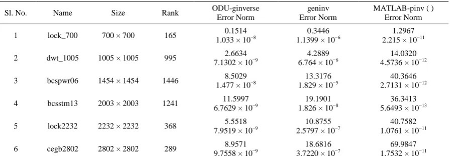
Table 1 and Table 2 records the times (in seconds) taken by our proposed algorithm, the algorithm mentioned

in [6] and MATLAB built-in function [7] pinv( ). For our convenience, we represent our algorithm with

( )

[image:4.595.92.540.407.566.2]

ODU−ginverse , algorithm in [6] with geninv and MATLAB built-in function with MATLAB−pinv( ). In addition, we have also presented the error norm for all the test matrices.

Table 1. Computational times (in seconds) for symmetric rank-deficient test matrices with RHS Vector as linear combina-tion of columns of coefficient matrix.

Sl. No. Name Size Rank ODU-ginverse Error Norm

geninv Error Norm

MATLAB-pinv ( ) Error Norm

1 lock_700 700 × 700 165 0.1514 1.033 × 10−8

0.3446 1.1399 × 10−6

1.2967 2.215 × 10−11

2 dwt_1005 1005 × 1005 995 2.6634 7.1302 × 10−9

4.2889 6.764 × 10−6

14.0320 4.5736 × 10−12

3 bcspwr06 1454 × 1454 1446 8.5029 1.477 × 10−8

13.3176 1.829 × 10−5

40.3646 2.7131 × 10−12

4 bcsstm13 2003 × 2003 1241 11.5997 6.7629 × 10−9

19.1901 1.826 × 10−8

36.3413 5.6493 × 10−13

5 lock2232 2232 × 2232 368 5.5518 7.9519 × 10−9

10.8755 2.5797 × 10−7

40.7582 1.0761 × 10−11

6 cegb2802 2802 × 2802 289 8.9571 9.7558 × 10−9

18.6816 3.7220 × 10−7

[image:4.595.87.539.605.721.2]

69.9847 1.7532 × 10−11

Table 2. Computational times (in seconds) for rectangular rank-deficient test matrices (Tall type: Rows >> Cols) with RHS Vector as linear combination of columns of coefficient matrix.

Sl. No. Name Size Rank ODU-ginverse Error Norm

geninv Error Norm

MATLAB-pinv ( ) Error Norm

1 D_6 970 × 435 339 0.1347 1.216 × 10−11

0.2809 1.333 × 10−11

1.3240 7.403 × 10−13

2 mk9-b2 1260 × 378 343 _{5.950 × 10}0.1162 −14 _{1.018 × 10}0.2478 −13 _{1.681 × 10}0.6098 −13

3 Franz1 2240 × 768 755 _{1.457 × 10}1.3077 −13 _{1.290 × 10}2.3649 −13 _{2.806 × 10}6.0490 −13

5. Conclusion

In this paper, various efficient algorithms for solving SLE with full rank, or rank deficient have been reviewed, proposed and tested. The developed numerical procedures can be applied to solve “general” SLE (in the form

[ ]

G

{ } { }

x = b , where the coefficient matrix

[ ]

G could be square/rectangular, symmetrical/unsymmetrical, non-singular/singular). The users have option to choose either a direct solver or an iterative solver inside the ge-neralized inverse to solve for SLE. Numerical results have shown that the proposed algorithms are highly

effi-cient as compared to existing algorithms [6] (including the popular MATLAB built-in function pinv G

( )

*b)

[7].

Acknowledgements

The authors would like to acknowledge Gelareh Bakhtyar for her useful discussions.

References

[1] Nguyen, D.T. (2006) Finite Element Methods: Parallel-Sparse Statics and Eigen-Solutions. Springer Publisher.

[2] Golub, G.H. and Loan, C.F.V. (1996) Matrix Computations. The John Hopkins University Press.

[3] Heath, M.T. (1997) Scientific Computing: An Introductory Survey. McGraw Hill Publisher.

[4] Hou, G. and Wang, Y. (2004) A Substructuring Technique for Design Modifications of Interface Conditions. Structur-al Dynamics & MateriStructur-als Conference, Palm Springs, California, 19-22 April 2004.

http://dx.doi.org/10.2514/6.2004-2010

[5] Farhat, C. and Roux, F.X. (1994) Implicit Parallel Processing in Structural Mechanics. Computational Mechanics Ad-vances, 2, Elsevier Publisher.

[6] Pierre, C. (2005) Fast Computation of Moore-Penrose Inverse Matrices. Neural Information Processing—Letters and Reviews, 8.

[7] MATLAB, MATLAB—The Language of Technical Computing. [8] Davis, T. University of South Florida Matrix Collection.