Forecasting intermittent demand

Lancaster University Management School

Working Paper

2006/027

Forecasting intermittent demand

Ruud Teunter and Laura Duncan

The Department of Management Science Lancaster University Management School

Lancaster LA1 4YX UK

© Ruud Teunter and Laura Duncan

All rights reserved. Short sections of text, not to exceed two paragraphs, may be quoted without explicit permission,

provided that full acknowledgement is given.

The LUMS Working Papers series can be accessed at http://www.lums.lancs.ac.uk/publications/

F

orecasting

I

ntermittent

D

emand

R

H.

T

D

M

S

L

U

M

S

LA1

4YX

L

,

UK

TEL

.

+0044

1524

592384

FAX

+0044

1524

844885

R

.

@

.

.

L

D

H

M

M

L

B

C

1-5

T

B

,S

P

S

,

S

A

,

H

,

UK

AL1

3LH

T

.

+0044

1727

855432

DUNCANL

@

.

.

Abstract

Methods for forecasting intermittent demand are compared using a large data-set from

the UK Royal Air Force (RAF). Several important results are found. First, we show

that the traditional per period forecast error measures are not appropriate for

intermittent demand, even though they are consistently used in the literature. Second,

by comparing target service levels to achieved service levels when inventory

decisions are based on demand forecasts, we show that Croston’s method (and a

variant) and Bootstrapping clearly outperform Moving Average and Single

Exponential Smoothing. Third, we show that the performance of Croston and

Bootstrapping can be significantly improved by taking into account that each lead

time starts with a demand.

1. Introduction

This study is motivated by the aim to increase the accuracy of forecasting and

inventory control of service parts at the Royal Air Force (RAF) in the UK. As is

typical of a service environment, most of the items in stock are slow-moving. The

bulk of the items are demanded less than five times per year and often much less. The

key problem in this case, and for inventory control of service parts in general, is that

of forecasting the mean and standard deviation of lead time demand. These forecasts

are needed to set the parameter(s) of the inventory control policy.

Forecasting lead time demand is complicated for slow-moving items, since limited

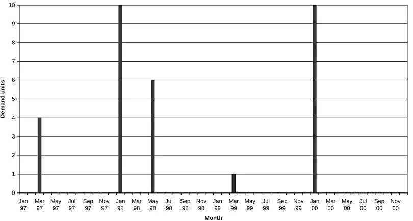
non-zero demand data is available. Figure 1 shows a typical example of the demand

pattern for the RAF. Note that even for a time bucket as large as a quarter of a year

(the RAF uses one month), the demand series often contain more zeros than positive

demands. Moreover, the positive demands vary considerably in size. Such an

intermittent demand pattern generally characterises slow-moving items.

Demand for an example item

0 1 2 3 4 5 6 7 8 9 10 Jan 97 Mar 97 May 97 Jul 97 Sep 97 Nov 97 Jan 98 Mar 98 May 98 Jul 98 Sep 98 Nov 98 Jan 99 Mar 99 May 99 Jul 99 Sep 99 Nov 99 Jan 00 Mar 00 May 00 Jul 00 Sep 00 Nov 00 Month Deman d u n it s

Figure 1. Typical monthly demand pattern for a slow-moving item

Because of these characteristics several authors, starting with Croston (1972), have

argued that the traditional forecasting methods such as moving average (MA) and

single exponential smoothing (SES, currently used by the RAF) are inappropriate and

by these authors and the results of comparative studies are discussed in detail. The

main methods proposed are: Croston’s original method, variants of Croston’s method,

and Bootstrapping. The results from comparative studies in the literature are

inconclusive. Though most studies conclude that the alternative methods perform

better on average, they often identify settings where the traditional methods perform

better. Some studies even find that the average performance of the traditional methods

is better.

In this paper, we show that these mixed findings originate (at least in part) from the

use of inappropriate performance measures. The most commonly used ‘per period

forecast error’ (again see Section 2 for details) is not informative for demand series

that consist of many zeros and few positive demands. Indeed, we will show, using a

large data-set from the RAF, that for this performance measure neither the traditional

nor the alternative methods outperform a simple benchmark method that always

forecasts zero. To the best of our knowledge, we are the first to include such a

benchmark and use it to show that per period forecast errors are inappropriate to

evaluate the performance of forecasting methods for intermittent demand.

A better way of comparing forecasting methods for slow-moving items is to analyse

their effect on inventory control parameters and to compare resulting inventory and

service levels. As described in Section 2, some authors have taken such an approach,

but their exact way of doing so sometimes hampers comparison. In this paper, we

develop a specific approach for comparing target service levels to actual service

levels.

We conclude from our comparison that, for the RAF data-set, the alternative methods

clearly outperform the traditional methods. Furthermore, we show how the alternative

methods can be significantly improved by exploiting the fact that a lead time always

starts with a positive demand. Although this seems straightforward, to the best of our

knowledge it has not been noticed and utilised in the literature.

The main body of the paper is organised as follows. In Section 2, the literature is

compare per period forecast errors of the benchmark method, traditional methods, and

Croston’s original method plus variants. In Section 5, we propose a bootstrap method

that is simpler and more practical than those previously suggested. In Section 6, we

compare the accuracy of all methods in attaining the target service level, and propose

a further improvement based on initial results. In Section 7, we end with conclusions.

2. Literature review on intermittent demand forecasting

As the focus of this paper is on forecasting, we do not review the literature on

inventory control rules for slow-moving items. Interested readers are referred to

Archibald and Silver (1978), Ward (1978) and Williams (1994).

Croston (1972) was the first to suggest that traditional forecasting methods such as

moving average (MA) and single exponential smoothing (SES) may be inappropriate

for slow-moving items. He demonstrated that they can lead to sub-optimal stocking

decisions and proposed an alternative forecasting procedure that separately updates

the demand interval and the demand size (exponentially, and with the same smoothing

constant for both), and only does so in periods with positive demand. The forecast for

the demand per period is then calculated as the ratio of the forecasts for demand size

and demand interval.

Modifications of the original Croston method were later proposed by several other

authors. Syntetos and Boylan (2001) argue that the original method is biased and

correct it by multiplying the forecast for the demand per period with 1−α /2, where α is the smoothing constant. Levén and Segerstedt (2004) use the Croston approach of only updating when there is a positive demand, but update the forecast for the

demand per period directly using the ratio of demand size and interval. They remark

that this method avoids the bias in the original Croston method as identified by

Syntetos and Boylan. Snyder (2002) introduces more complex variations of the

Croston method, which involve bootstrapping.

Bootstrapping has also been proposed by Porras Musalem (2005) and Willemain et al.

lead time demand distribution is forecasted directly by repeated sampling from

realised demands. This technique is in contrast to all previously discussed methods,

which first forecast the demand per period, and take this as the mean while the

variance is based on past forecast errors. There are many variants of the bootstrapping

method. Interested readers are referred to Bookbinder and Lordahl (1989) and Efron

(1979). A disadvantage of many is that they are rather complex. This also holds for

the bootstrapping method proposed by Willemain et al. (2004). It involves estimating

transition probabilities in a Markov model and using that model to generate a

sequence of zero/non-zero demand values. The bootstrapping method proposed by

Porras Musalem (2005) is simpler. Moreover, it can capture demand autocorrelation

by restrictive sampling. However, that does imply that it cannot ‘maximise the use’ of

the limited available data. Since there is no significant autocorrelation for the RAF

case, we use a different bootstrapping method in this study (see Appendix A for a

detailed description).

Comparative studies

The traditional forecasting methods have been compared to (variants of) the Croston

method in a number of studies (Eaves, 2002; Eaves and Kingsman, 2004; Ghobbar

and Friend, 2003; Johnston and Boylan, 1996a; Johnston and Boylan, 1996b; Levén

and Segerstedt, 2004; Regattieri et al., 2005; Sani and Kingsman, 1997; Syntetos and

Boylan, 2005; Willemain et al., 1994). Essentially, two types of performance

measures are used. The first type is the most common and compares per period

forecast errors, usually measured by the mean absolute deviation (MAD), mean

square error (MSE), or mean absolute percentage error (MAPE). The second type

transforms the forecasts into the stock control parameter(s) and compares the average

inventory and/or service levels.

The second type of performance measures can be implemented in many different

ways. In fact, all papers that use this type, implement it in a different way. Eaves and

Kingsman (2004) initially set the safety stock to zero and determine the maximum

backlog for the corresponding reorder level. They then raise the reorder level by the

maximum backlog amount so that a 100% service level is achieved, and calculate the

lead time variance forecast plays no role and (ii) a 100% service level can never be

achieved in practice. Sani and Kingsman (1997) calculate the percentage increase in

average inventory/service level of a method compared to the method with the lowest

level. The disadvantage here is that a low inventory level automatically implies a high

service level, and hence that no clear decision is possible on which method performs

best. Levén and Segerstedt (2004) propose calculating a combination of average

service level and inventory level for many different reorder levels and compare the

inventory-service curves. These curves do allow a clear decision if one curve is closer

to the axis than another. However, they do not show the difference between the target

service level and the actual service level.

Although the exact implementation of the second type of performance measure

sometimes hampers comparison (as discussed above), most results indicate that

Croston-type methods outperform traditional methods. The comparative studies

(mainly) based on per period forecast errors have led to a mixed bag of results.

Almost no study finds consistent superior performance (for all considered settings)

from either Croston-type or traditional methods. Most studies do conclude that

Croston-type methods perform better on average, but some find the opposite.

As for the performance of bootstrapping methods, Willemain et al. (2004) conclude

that their method produces more accurate forecasts of lead time demand (based on

assessing the uniformity of observed percentiles, pooled across items, in a rather

complex way) than exponential smoothing and Croston’s original method. The results

of the same comparison by Snyder (2002), for his complex variations of the Croston

method involving bootstrapping, are unclear, partly due to the small number of items

in his data-set. Porras Musalem’s (2005) comparison is restricted to bootstrapping

methods. He compares two variants of his own method, fitting a normal distribution

to the empirical mean and variance or using the ‘full’ empirical distribution, to

themethod of Willemain et al. He concludes that both variants outperform the method

3. Case study (data) details

The data are sampled from demand for consumable spare parts – i.e. spare parts with

no associated repair activity - as used by the RAF. The items are all classified as

intermittent and lumpy – that is, they show demand patterns such as that in Figure 1.

The spare parts include, for example, valves, diodes, screws and cables.

The data-set included 5000 items and covered 6 years (1997-2002). Items are selected

randomly from those that had at least one demand in this time period. The lead time

for each item, including the production lead time and the administration lead time, is

available. Both lead time components are fairly constant, and therefore the lead times

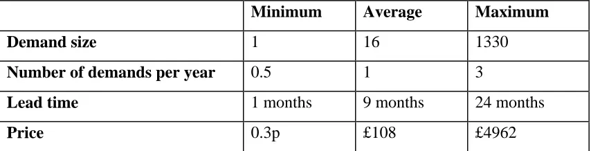
are assumed to be deterministic. Relevant characteristics of the data are summarised

in Table 1.

Minimum Average Maximum

Demand size 1 16 1330

Number of demands per year 0.5 1 3

Lead time 1 months 9 months 24 months

Price 0.3p £108 £4962

Table 1. Information about the data-set for the first four years.

A distinction between slow-moving, intermittent and irregular demand, as suggested

by Eaves and Kingsman (2004), was considered, but was not made because the data

was not found to divide naturally or usefully into any such categories. In

slow-moving demand forecasting it is also usual to assume the absence of any seasonality

or complicated trends, due to the lack of any evidence for these factors in series with

4. Methods that are included in the comparative study

The methods that we include in our study are listed below, with the abbreviations

used for them and journal and textbook references in which they are described.

Name of method Abbrev. Reference

Zero forecast ZF n/a

Simple moving average MA Makridakis et al, 1998, pp142

Exponential smoothing ES Makridakis et al, 1998, pp147

Croston’s method CR Croston, 1972

Syntetos-Boylan variation of Croston’s method

(elsewhere referred to as the Approximation

method)

CR_SB Syntetos and Boylan, 2001

Eaves and Kingsman, 2004

Levén-Segerstedt variation of Croston’s method CR_LS Levén and Segerstedt, 2004

Bootstrapping BS Bookbinder and Lordahl, 1989

The Zero Forecast method is the benchmark technique against which all others are

compared. For this method a demand prediction of zero is made for each month.

This method is expected to be the worst technique, since such a forecast is of no value

for inventory control. To the best of our knowledge, the inclusion of a benchmark

method has not been considered in the literature. As the next section will show, it

enables firmer comparisons to be drawn.

For practicality, the bootstrapping method that we use is much simpler than that

proposed by Willemain et al. (2004). For the same reason, we do not include the

complex Croston variants proposed by Snyder (2002).

Details of all other methods are provided in Appendix A. There, we also describe why

we set the smoothing constant to 0.15 for all methods that use smoothing (though we

5. Traditional performance measures

This section illustrates that traditional performance measures of forecast error per

period cannot be used for comparing methods of forecasting intermittent demand,

even though that has repeatedly been done in the literature, as discussed in Sections 1

and 2.

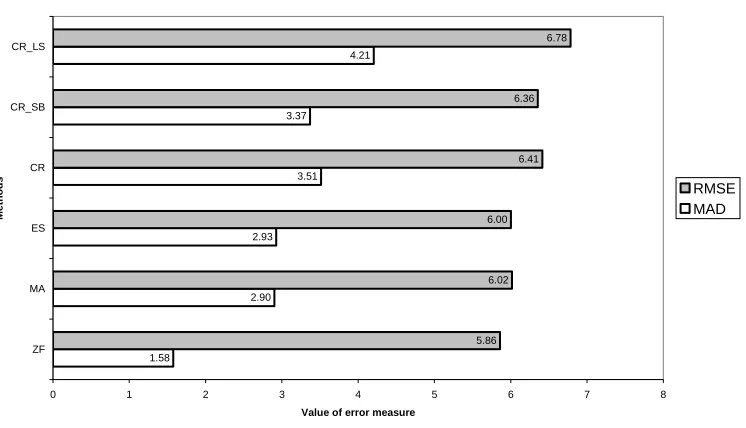
Figure 2 shows the results for the Mean Absolution Deviation (MAD) and the Mean

Squared Error (MSE), which were used in previous studies on intermittent demand

(Eaves and Kingsman, 2004; Regattieri et al., 2005; Sani and Kingsman, 1997;

Syntetos and Boylan, 2005). Note that, for ease of presentation, Figure 2 displays the

Root Mean Squared Error (RMSE) instead of the MSE.

Results for MAD and RMSE for all appropriate methods

4.21

1.58

2.90 2.93

3.51 3.37

5.86

6.78

6.36

6.41

6.00

6.02

0 1 2 3 4 5 6 7 8

ZF MA ES CR CR_SB CR_LS

Me

tho

d

s

Value of error measure

RMSE MAD

Figure 2. MAD and RMSE error measures.

A sensitivity analysis, where the smoothing constant is varied within the 0.1-0.2

range, reveals that these results are robust. The smoothing constant does have some

effect on the performance of methods, but this effect is small in comparison to the

difference in performance between the various methods.

Similar results are obtained (but not reported in detail here) for the Relative

recommended by Eaves and Kingsman (2004) and used by Syntetos and Boylan

(2005), following research by Fildes (1992).

The Mean Absolute Percentage Error (MAPE) is not employed, despite some studies’

use of it (Eaves and Kingsman, 2004). The argument against MAPE, as explained by

Willemain et al. (2004), is that the calculation requires division by the demand, and

for slow-moving demand the series will include a large number of zero demand

points.

Discussion of results

The main, and striking, result is that the Zero Forecast comes out as the best of all the

methods. Though surprising at first, this result is logical and is illustrated by the

following simple example. If demand is 0 for nine out of ten months and the average

demand size is 10 when a demand does occur, then the zero-forecast will have an

MAD of , whereas the ‘correct’ per period forecast

of 1 will have an MAD of

(

)

(

)

(

)

(

)

(

)

(

)

MAD calculation. This argument also explains why the Croston-type methods have

higher MADs than MA and SES, since the traditional methods adjust the forecast

towards zero after each period of zero demand. The same arguments hold for the

(R)MSE and GRMSE, although to a lesser extent.

This result does not imply that the MA and SES are preferable to Croston-type

methods, and certainly does not imply that it is even better to use the ZF. It means,

rather, that per period forecast errors are not appropriate error measures in this area.

In the context of inventory control, what matters is whether a forecast and

corresponding forecast error result in the distribution of lead time demand being well

approximated. In the next section, we therefore transform these distributions to

inventory decisions and compare methods in their ability to approximate the target

6. Service Level Accuracy

The general logic of looking at the Service Level Accuracy is to compare a target

service level to the actual service level achieved when inventory control parameters

are based on the demand forecasts from given forecasting methods. It can be used for

any type of inventory policy and any definition of service level, as long as there is a

way of calculating control parameters from the forecasts.

We focus on the order-up-to policy, which is used by the RAF and generally accepted

as an appropriate method for controlling slow-moving inventory. The cycle service

level definition is used, i.e. the service level is equal to the fraction of orders that

arrives on time. We further assume that lead time demand is normally distributed. As

shown in Appendix B, the normal distribution provides a reasonable fit for the RAF

data-set. Using the forecasts for the mean and standard deviation of lead time demand

(generated by selected methods, see below), the calculation of the order-up-to level is

by straightforwardly using the inverse normal distribution function.

Bootstrapping (BS) directly produces forecasts for the mean and standard deviation of

lead time demand by repeatedly and randomly drawing L (lead time) realisations of

past monthly demand (see Appendix A for details).

All other methods produce a forecast for the demand per period and the associated

forecast error. Using these outputs, the mean lead time demand is determined as the

product of the per period forecast and L, and the standard deviation can be calculated

as the product of the Root Mean Square Error (RMSE) and L. This is the common

approach for transforming per period forecasts into lead time forecasts.

We remark now that later on in this section, we will propose modified approaches for

the BS, as well as the other methods, based on initial results. We further remark that

Levén and Segerstedt provide an alternative variance estimator, which we do not use,

in order to get a clear comparison.

Recall from Section 3 that the RAF data-set covers a six year period. For each

deviation of lead time demand, where the initial year is used for initialisation for all

methods (except bootstrapping where no initialisation is necessary). This initialisation

needs some further explanation, as it is not always straightforward. For MA and SES,

the initial demand forecast is the average monthly demand over the initial year. For

the Croston-type methods, (i) the initial forecast of the demand size is the

straightforward average if at least one demand has occurred, and is otherwise set to 1;

(ii) the initial forecast of the demand interval is the straightforward average if at least

two demands (and hence one interval) have occurred, and is otherwise set to 12

months. This is in line with proposals from Eaves (2002) and Willemain et al. (2004).

The latter two years of the data-set are then used to evaluate whether the

order-up-to-levels lead, approximately, to the required service level (starting with no items on

order at the start of this two year period). It is important to note that we can only

expect a close approximation as an average over a large group of items. To see why,

consider an item for which 3 orders are placed over the evaluation period. For that

item, the cycle service level over the evaluation period can only be 0%, 33%, 67% or

100%. A target service level of, say, 95% could therefore never be too closely

approximated for this single item.

Results

In a military context, loss of service level is entirely inappropriate and high service

levels are required. Therefore, only service levels above 90% are chosen for testing.

Despite this decision, testing the accuracy of the predicted distributions could, in

principle, be carried out with any service levels.

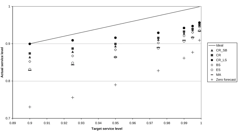
The results are summarised in Figure 3. We remark that a sensitivity analysis showed

these results to be robust to changes in the smoothing parameter. Note that the actual

service level increases with the target service for Zero Forecast (and all other forecast

Service Level Accuracy

0.7 0.8 0.9 1

0.89 0.9 0.91 0.92 0.93 0.94 0.95 0.96 0.97 0.98 0.99 1 Target service level

A c tu al se rvice leve l Ideal CR_SB CR CR_LS BS ES MA Zero forecast

Figure 3. Comparison of Service Level Accuracy for the different forecasting

methods. Results are averaged over all items.

Zero Forecast is definitely the worst method – as anticipated. Moving Average and

Single Exponential Smoothing perform fairly similarly to each other. Bootstrapping

performs better, but is in its turn outperformed by all Croston-type methods. Among

the Croston-type methods: the Levén-Segerstedt variation has the best performance,

followed by original method that performs slightly better that the Syntetos-Boylan

variation.

Another important result is that all methods lead to service levels that are significantly

below their targets (as shown by comparison to the Ideal series). A reason for this

could be that the normal distribution provides a very poor fit for lead time demand, in

particular that it underestimates the pth quantile for the entire range

considered. However, as is shown in Appendix B for two randomly selected items

(other items show similar results) using the results of bootstrapping, this is not the

case. In fact, the p

] 1 , 9 . 0 [ ∈ p th

quantile is overestimated for values up to about 0.95.

So, if the non-normality is not the (main) cause for actual levels being consistently

below their targets for all methods, then apparently the mean and/or variance of lead

following explanation: all methods ignore the fact that an order is triggered by a

demand, and therefore ignore that a lead time starts with a demand. Obviously, doing

so can lead to a serious underestimation of the mean lead time demand. In the next

section, we will therefore propose a modification to the calculation of that mean and

show that this indeed significantly improves the performance.

Adjusting the mean lead time demand

As explained above, we want to adjust lead time demand to take into account of the

fact that each lead time starts with a demand. For bootstrapping (see Appendix A for

details), this is done by requiring the first of L draws to be chosen from those months

with positive demand. For Croston’s original method and the Syntetos-Boylan

variation, the adjusted mean lead time is equal to the demand size forecast for the first

month plus L-1 times the demand per period forecast. Recall that it used to be L times

the demand per period forecast. Note that a similar adjustment cannot be made for

MA, SES, and CR_LS, since those methods do not forecast demand size and demand

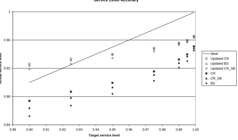
Figure 4 compares the performance of the original methods to the adjusted methods.

Service Level Accuracy

0.84 0.88 0.92 0.96 1

0.89 0.90 0.91 0.92 0.93 0.94 0.95 0.96 0.97 0.98 0.99 1.00 Target service level

A

c

tu

al se

rvice leve

l _Ideal

Updated CR Updated BS Updated CR_SB CR

CR_SB BS

Figure 4. Increase in Service Level accuracy due to a modified calculation of mean

lead time demand (scale different from Figure 3). Results are averaged over all

items.

As can be seen from Figure 4, the improvement in performance is significant. Note

also that the actual service level is no longer consistently below the target service

level. For target service levels below ca 94% (for these two items) the actual service

level is still lower, but for target service levels above 94% the actual service level is

higher. As discussed in the previous section, this can be explained by the use of the

normal distribution for fitting the lead time demand distribution.

This suggests that further improvement may be possible by assuming a different

distribution of lead time demand, or for the Bootstrapping method by directly using

the ‘full’ distribution determined by bootstrapping. As explained in Appendix A, the

latter suggestion also has a major disadvantage: it can lead to jumps in the considered

7. Conclusion

By comparing both basic (MA, SES) and Croston-type forecasting methods to a

simple benchmark method that always generates a zero forecast, we clearly showed

that traditional per period forecast errors are inappropriate for measuring the

performance of forecasting methods for items with intermittent demand. To the best

of our knowledge, we are the first to include such a benchmark policy and obtain this

insight. Indeed, it explains to a large extent why the literature has been inconclusive

with respect to the question of whether Croston-type methods indeed outperform

general methods.

Building on some suggestions in the literature, we proposed to measure performance

by comparing target service levels to actual service levels. Doing so for a large

data-set from the RAF showed that Croston-type methods significantly outperform general

methods. We also included a bootstrap method in the comparative study, which

performed slightly worse than the Croston-type methods but still considerably better

than the general methods.

Based on the observation that actual service levels were consistently below their

targets for all methods, we suggested a modification in the determination of

order-up-to levels by taking inorder-up-to account that each lead time starts with the demand that

triggers it. Although this seems straightforward, to the best of our knowledge it has

not been suggested in the literature previously. The modification significantly

improves the performance of the original Croston method, the Syntetos-Boylan

variation and the bootstrap method. The other methods cannot be modified in this way

as they do not separately forecast the demand size and the demand interval.

The results for these modified order-up-to levels suggest that the remaining service

level inaccuracy is largely explained by the deviations of the actual lead time

distribution from the Normal distribution. So, further improvement may be possible

by considering other distributions (e.g. Erlang), or for Bootstrapping by using the full

empirical distribution rather than the first two moments. This, however, requires

Based on the results of this research, we advocate the use of the original Croston

method with modified calculation of order-up-to levels. Bootstrapping performs

equally well, but is more difficult to implement.

References

Archibald BC and Silver AE (1970). (s,S) policies under continuous review and

discrete compund Poisson demand. Management Science, 24, 899-904.

Bookbinder JH and Lordahl AE (1989). Estimation of inventory re-order levels using

the bootstrap statistical procedure. IIE Transactions, 21, 302-312.

Croston JF (1972). Forecasting and stock control for intermittent demands.

Operational Research Quarterly, 23, 289-304.

Eaves AHC (2002). Forecasting for the ordering and stock-holding of consumable

spare parts. PhD thesis, University of Lancaster, UK.

Eaves AHC and Kingsman BG (2004). Forecasting for the ordering and

stock-holding of spare parts. Journal of the Operational Research Society, 55, 431-437.

Efron B (1979). Bootstrap methods: Another look at the jackknife. Annals of

Statistics, 7, 1-26.

Fildes R (1992). The evaluation of extrapolative forecasting methods. International

Journal of Forecasting, 8, 81-98.

Ghobbar AA and Friend CH (2003). Evaluation of forecasting methods for

intermittent parts demand in the field of aviation: a predictive model. Computers

and Operations Research, 30, 2097-2114.

Johnston FR and Boylan JE (1996). Forecasting for items of intermittent demand.

Journal of the Operational Research Society, 47, 113-121.

Levén E and Segerstedt A (2004). Inventory control with a modified Croston

procedure and Erlang distribution. International Journal of Production

Economics, 90, 361-367.

Makridakis S, Wheelwright SC and Hyndman RJ (1998), Forecasting: Methods and

Applications, 3rd edition, John Wiley & Sons, Inc., New York

Porras Musalem E (2005). Inventory Theory in Practice: joint replenishments and

spare parts control (Chapter 6), PhD thesis Erasmus University Rotterdam

Regattieri A, Gamberi M, Gamberini R and Manzini R. (2005). Managing lumpy

demand for aircraft spare parts. Journal of Air Transport Management, 11,

426-431.

Sani B and Kingsman BG (1997). Selecting the best periodic inventory control and

demand forecasting methods for low demand items. Journal of the Operational

Research Society, 48, 700-713.

Syntetos AA and Boylan JE (2001). On the bias of intermittent demand estimates.

International Journal of Production Economics, 71, 457-466.

Syntetos AA and Boylan JE (2005). The accuracy of intermittent demand estimates.

International Journal of Forecasting, 21, 303-314.

Ward JB (1978). Determining reorder points when demand is lumpy. Management

Science, 24, 623-632.

Willemain TR, Smart CN and Schwarz HF (2004). A new approach to forecasting

intermittent demand for service parts inventories. International Journal of

Forecasting, 20, 375-387.

Willemain TR, Smart CN, Shockor JH and DeSautels PA (1994). Forecasting

intermittent demand in manufacturing: a comparative evaluation of Croston’s

method. International Journal of Forecasting, 10, 529-538.

Williams TM (1982). Reorder levels for lumpy demand. Journal of the Operational

Research Society, 33, 185-189.

Acknowledgements

This paper is based on a project sponsored by Logistics Analysis and Research

Organisation (LARO), a sub-department of the Defence Logistics Organisation

(DLO), based in Wyton, UK. In particular, we thank David Hampton, Robert

Appendix A. Forecasting methods

Table A.1 lists the notations used in this appendix.

Notation Definition

$

d_t Forecast for mean demand per period after period t

d_t Realised demand in period t

n_t Number of time units since the previous demand occurred (if a demand occurs in period t)

$

s_t Forecast for mean demand size after period t (Croston-type methods)

$

n_t Forecast for the demand interval after period t (Croston-type methods)

α Smoothing parameter (SES and Croston-type methods)

m Demand history on which the forecast is based (MA)

L Lead time

Table A.1. Notations

Table A.2 gives the mathematical details of all considered forecasting methods except

bootstrapping.

Name demand size

$

s_t

demand interval

$

n_t

demand per period

$ d_t

Moving Average --- --- 1

0 1

m k dt k

m − = −

∑

--- --- α _dt + −₍₁ α_)d$_t−1

Croston

Original

αdt +(1−α)s$t−n_t αnt + −(1 α)n$t−n_t $

$ s n t t Croston

Syntetos & Boylan

αd_t α s_t t

+(1− )_$−n αn_t α n_t

t n

+ −(1 )_$−

t t n s ˆ ˆ 2 1 ⎟ ⎠ ⎞ ⎜ ⎝

⎛ −α

Croston

Levén & Segerstedt

--- ---

α d α

n d

t

t

t nt

+ −(1 )$−

Table A.2. Details of forecasting methods included in out comparative study (except

Values of between 0.1 and 0.3 for the smoothing constantα are generally accepted to

make SES work successfully. For Croston-type methods, several suggestions have

been made. Croston (1972) recommends 0.2 < α < 0.3 when a high proportion of

items have non-stationary, intermittent demand, but 0.1 < α < 0.2 otherwise.

Syntetos and Boylan (2001) suggest that α should be no more than 0.15. Eaves

(2002) chooses values in the range of 0.01-0.1. As a compromise between these

conflicting suggestions, we use a smoothing constant of 0.15. Moreover, we use the

same constant for all Croston-type methods and for SES to ensure a fair comparison.

For MA, we set the demand history m on which the forecast is based to 12, i.e. the

demand history is one year.

Bootstrapping

Bootstrapping techniques estimate the (moments of the) distribution of lead time

demand by repeatedly sampling L demands from the demand history. The sampling

can be done in many different ways. Especially, one can sample with or without

replacement, and sample randomly or restricted to successive months. To maximise

the use of the limited available data involved with mostly zero demand series, we

choose to sample with replacement and randomly. We sampled 10,000 times, as that

turned out to be sufficient for obtaining stable estimates.

We use the bootstrapping results to calculate the mean and standard deviation of lead

time demand for an item. The order-up-to level is then determined by assuming a

normal distribution, as is done for all other methods. Alternatively, the ‘full’

distribution resulting from bootstrapping could have been used to determine the

order-up-to level. However, the full distribution can be far from smooth if there are very

few demand occurrences. For instance, based on two demand occurrences of sizes 5

and 6, respectively, the full distribution would suggest that possible lead time demand

values are restricted to 0, 5, 6, 10, 11, 12, 15, etc., which would imply that only these

Appendix B. Normality of lead time demand

In Figures B.1 and B.2, the lead time distribution resulting from bootstrapping is

compared to the (discrete) normal distribution with the same mean and variance for

two randomly selected items (numbered 1 and 2, respectively, in this appendix).

0 200 400 600 800 1000 1200 1400 1600

1 2 3 4 5 6 7 8 9 10 11 12 13 14 15 16 17 18 19 20 21

Lead time demand

Number of

sampl

es

wit

h

each

demand

Observed data Normal curve

Figure B.1. The observed lead time (17 months) demand distribution from

bootstrapping versus the Normal distribution with the same mean and variance for

item 1.

0 500 1000 1500 2000 2500 3000 3500

1 2 3 4 5 6 7 8 9

Lead time demand

Number

of samples w

ith

each deman

d

Observed data Normal distribution

Figure B.2. The observed lead time (8 months) demand distribution from

bootstrapping versus the Normal distribution with the same mean and variance for

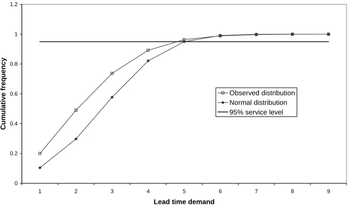
The main conclusion for these two items (and for other items as well) is that the

normal curve provides a reasonably good fit to the observed data, although it

somewhat overestimates the probabilities of large demands and underestimates the

probabilities of very large demands. This is further illustrated by the cumulative

relative frequency curves in Figures B.3 and B.4, which show that for these two items

the observed and normal curves intersect around the 95% cumulative relative

frequency / probability point, corresponding with the 95% cycle service level.

0 2000 4000 6000 8000 10000 12000

1 2 3 4 5 6 7 8 9 10 11 12 13 14 15 16 17 18 19 20 21

Lead time demand

C

u

m

u

lat

ive frequency

Observed distribution Normal distribution 95% Service Level

Figure B.3. Cumulative frequency curves for item 1.

0 0.2 0.4 0.6 0.8 1 1.2

1 2 3 4 5 6 7 8 9

Lead time demand

Cum

u

la

tiv

e

freq

uen

c

y

Observed distribution Normal distribution 95% service level

Note from a comparison of Figures B.1 (B.3) and B.2 (B.4) that a larger lead time

results in a smoother distribution from bootstrapping. The same effect also results