Foundations for Wash Sales

http://www.scirp.org/journal/jmf ISSN Online: 2162-2442 ISSN Print: 2162-2434

Foundations for Wash Sales

Phillip G. Bradford

Department of Computer Science and Engineering, University of Connecticut, Stamford, CT, USA

Abstract

Consider an ephemeral sale-and-repurchase of a security resulting in the same posi-tion before the sale and after the repurchase. A sale-and-repurchase is a wash sale if these transactions result in a loss within ±30 calendar days. Since a portfolio is essen-tially the same after a wash sale, any tax advantage from such a loss is not allowed. That is, after a wash sale a portfolio is unchanged so any loss captured by the wash sale is deemed to be solely for tax advantage and not investment purposes. This pa-per starts by exploring variations of the birthday problem to model wash sales. The birthday problem is: Determine the number of independent and identically distri-buted random variables required so there is a probability of at least 1/2 that two or more of these random variables share the same outcome. This paper gives necessary conditions for wash sales based on variations on the birthday problem. Suitable vari-ations of the birthday problem are new to this paper. This allows us to answer ques-tions such as: What is the likelihood of a wash sale in an unmanaged portfolio where purchases and sales are independent, uniform, and random? Portfolios containing options may lead to wash sales resembling these characteristics. This paper ends by exploring the Littlewood-Offord problem as it relates capital gains and losses with wash sales.

Keywords

Wash Sales, Tax, Birthday Problem, Littlewood-Offord, Probability, Finance

1. Introduction

Wash sales occur when a security is sold and quickly bought back with the sole intent to capture a tax loss from the sale. Wash sales impact a portfolio’s tax liabilities. Deter- mining the likelihood of wash sales is also important for understanding investment strategies and for comparing actively and passively managed portfolios. Wash sales apply to investors, but not to market makers.

How to cite this paper: Bradford, P.G. (2016) Foundations for Wash Sales. Journal of Mathematical Finance, 6, 580-597. http://dx.doi.org/10.4236/jmf.2016.64044

Received: June 13, 2016 Accepted: October 14, 2016 Published: October 17, 2016

Copyright © 2016 by author and Scientific Research Publishing Inc. This work is licensed under the Creative Commons Attribution International License (CC BY 4.0).

http://creativecommons.org/licenses/by/4.0/

581 Taxes play a significant role in economics and finance. Taxes influence behavior, shape the engineering of financial transactions, and sometimes have unintended consequences. Therefore, thoughtful analysis is imperative for taxes. This paper adds firm mathematical foundations to aid the understanding of wash sale taxes.

The main goal of this paper is: To provide foundations for certain wash sales-in cases when they may occur as well as the capital gain implications. This may also help differentiate managed funds and unmanaged index funds in terms of wash sales.

Wash sales are sometimes created by the exercise of options, thus a portfolio manager may not be able to avoid a wash sale in some contexts. For example, suppose an in-the-money American-style put option is written in a portfolio. Provided this option remains in-the-money, it may be exercised by its holder1 _{at anytime up to its}

expiry. If the exercise of this put option replaces shares sold at a loss in the prior 30 days, then this is a wash sale. This option’s exercise is beyond control of the portfolio manager.

The foundations given here start with variations of the classical birthday problem from probability theory [1]-[3]. This work has implications on wash sales. Also, the Littlewood-Offord problem [4]-[6] is applied to understand capital gains for certain wash sales. The Littlewood-Offord problem is viewed from the perspective of the pro- babilistic method.

For convenience, let

[ ]

n ≡

{

1, 2,,n

}

.

1.1. Wash Sales in Detail

Suppose a security is sold at a loss on day d2. This sale is a wash sale if substantially the same security is purchased within ±30 calendar days from d2, see for example

[7].

Definition 1 (US wash sale [7]) Consider three dates d d d1, 2, 3:d1≤d2 and d1≤d3 where d3−d2 ≤30 calendar days. Suppose s shares of a security are purchased on date d1 at price p1. At some later date d2, s shares are sold for price p2< p1. Thus, the s shares are sold at a loss. Then within ±30 days on date d3, s shares are repurchased for price p3. This is a wash sale and since d3−d2 ≤30 days, then the next adjustments must be made [7]:

1) The loss p1−p2 is not permissible for taxes. That is, this loss may not be subtracted from profits or gains and it may not be used to get a lower tax rate.

2) The cost-basis of the shares repurchased on d3 is set to p3+

(

p1−p2

)

. The shares purchased on d3 have the start of their holding period reset to d1.

Short positions may also be wash sales. For example, consider holding a short position of 100 shares of a security starting on date d1 in a portfolio Π. Then suppose this short position is closed at a loss by purchasing 100 shares on day d2. Once this position is closed on day d2, then Π contains no shares of this security. Next re-short another 100 shares of substantially the same security on d3 where

3 2 30

d −d ≤ days. These transactions leave the portfolio the same while getting a tax

advantage for the loss. This tax advantage is also disallowed by the wash sale rules. Consider a wash sale as described by Definition 1, where

(

p1−p2

)

+p3 > p1 or in other words p3> p2. Suppose the shares are sold at price p4>

(

p1−p2

)

+ p3> p1 at the later date d4≥d3. In the case with the wash sale, there is a capital gain of

(

)

4 1 2 3

p −_ p −p +p _ which is smaller than the capital gain p₄−p₁ if the wash sale

had not occurred. Capital gains are taxable. A capital gain p4−p1 is from the single purchase of the shares for price p1 on d1 and the single sale of the shares on date

4

d for price p4, thus skipping the sale at a loss and repurchase.

This means such a wash sale gives p4−p1−p4 −

(

p1−p2

)

+p3 or p3−p2 less taxable income than a single purchase of the security at price p1 on date d1 and a single sale for price p4 on d4. Of course, a wash sale’s loss is not allowed.

Wash sales may be avoided by restricting each security in a portfolio to be either purchased or sold only every 31 calendar days. This restriction may not be suitable for many portfolios. In a portfolio containing options, it may be impossible to maintain this restriction.

It has also been suggested, e.g. [9], wash sales may be avoided by purchasing or selling (moderately) correlated, but not substantially the same, securities. That is, if a security is sold at a loss then purchase a different but correlated security within 30 days maintaining some of a portfolio’s characteristics while keeping the tax advantage.

Historically many securities are assumed to only trade on about n=252 business

days per year [10]. Although reflecting on global markets one may assume there are

365

n= trading days.

1.2. Background

There has not been much research on wash sales, e.g., [9]. There is important work on taxation and its investment implications. Take, for example, [11]-[13].

The birthday problem is classical.

Definition 2 (Birthday-Collision) Given two random variables X X1, 2 mapping respectively to x x1, 2 in the same range

[ ]

n , then a birthday-collision is when x1=x2.

To model random wash sales, this paper assumes independent identically distributed random variables. A common statement of the birthday problem is:

Definition 3 (Birthday Problem) Consider n days in a year and k independent identically distributed (iid) uniform random variables whose range is

[ ]

n and n≥k.

What is the probability B n k

( )

, of at least one birthday-collision among these k

random variables?

According to a blog post by Pat B [14] the birthday problem may have originally been given by Harold Davenport as cited in [15] and later published by [1]. In any case, von Mises gave the first published version to the best of our knowledge.

583 distance d for cyclic years are given by [17].

The birthday problem applied to boys and girls (random variables with different labels) are discussed in [18] as well as [19]. That is, how many birthdays are shared by one or more boys and one or more girls? A comprehensive view is provided by [20]

including stopping problems with the boy-girl birthday problem. Non-uniform bounds for online boy-girl birthday problems are given by [21] and [22].

Tight bounded Poisson approximations for birthday problems are given by [23]. Poisson approximations to the binomial distribution for the boy-girl birthday problem is given by [19]. A Stein-Chen Poisson approximation is used by [24] to solve variations of the standard birthday problem. Matching and birthday problems are given by [25]. Incidence variables are used to study birthday problems with Pareto-type distributions in [26].

Applications of the birthday problem include: computer security [20][21][26][27], public health and epidemiology [28], psychology, DNA sequence alignment, experi- ments, and games [29] [30]. Summaries of work on the birthday problem are in [29]- [31].

Results on the expectation for getting j different letter k-collisions are given by [32]. Their results are expressed as truncated exponentials or gamma functions.

The Littlewood-Offord problem hails from complex analysis [6]. Erdös [5] improved Littlewood and Offord’s result by an elegant application of the probabilistic method. These and related results determine the concentration of sums of random variables multiplied by integers. The Littlewood-Offord problem is applied to certain capital gains.

1.3. Structure of This Paper

Section 2 reviews variants the birthday problem applied here. First the classical birthday problem is discussed. Next this section progresses through the ±d birthday problem.

After the definition and key results are given about the ±d birthday problem, the

boy-girl birthday problem is explored. Finally, the ±d boy-girl birthday problem is

defined and several bounds are derived as they relate to a necessary condition for wash sales.

Subsection 2.1 gives an example of wash sales based on boy-girl birthday collisions of a single day.

Section 3 generalizes results of the previous sections. In particular, it shows how to compute Bd

(

n b g, ,

)

, the number of b boys and g girls that give a probability of 1/2 or

more where a boy and a girl have birthdays within d days of each other over n days. Subsection 3.1 gives an example of wash sales based on boy-girl birthday collisions over a range of ± =d 30 days.

2. The Birthday Problem and Wash Sales

The birthday problem is often applied to finding the probability of coincidences. So there is a rich literature on variations of the birthday problem [29][30]. Asset sales are often viewed as carefully selected. However, portfolios using American-style options may exhibit asset sales or purchases beyond the control of the portfolio managers.

A key question is: Over n consecutive days for what integer k does

( )

1

arg min ,

2

k B n k

 _≥ 

 

  hold for k iid uniform random variables? In other words, given n days, what is the least k iid uniform random variables so that B n k

( )

, =1 2?

Solutions to this basic variation of the birthday problem are well known. The probability B n k

( )

, is the compliment of the probability of k iid uniform random

variables having no birthday-collisions. Therefore, if there are no birthday-collisions, then k birthdays can be in n k!

k

   

  permutations out of all possible

k

n mappings of

the k random variables onto

[ ]

n . In other words, the n

k

   

  subsets of k distinct

elements of

[ ]

n is the exact number of subsets the k variables may map to without a

collision. These k variables may be ordered in k! permutations. That is,

( )

!

₍

!

₎

1

, 1 1 ,

!

k k

n k n

B n k

k n n k n

 

= −_{ } = − ⋅

−

  (1)

for n≥k and B n k

( )

, =1 otherwise.

Starting with n and a probability p=B n k

( )

, , then computing k is often done using

the inequality 1 e x

x −

− ≤ _{. In particular, the smallest k giving a probability of 1/2 that} there is at least one birthday-collision requires k to be roughly 2 ln 2

( )

n or about 1.18 n. See for example, [1][33][34].

Another classical approach is to look at the random variable X as the sum of all birthday-collisions of k people over n days, see for example [19] [25] [35] [36]. A concise exposition is given in [36] which we follow. Presume the birthday of person

[ ]

i∈ k is given by the random variable Yi∈

[ ]

n . Since a potential birthday collision is a Bernoulli trial, so X is binomially distributed. Thus, 0,1, 2, ,

2

k X∈   _{ }

  

   where

2

k

   

  is the maximum number of potential birthday-collisions. The expectation of the

maximum number of birthday collisions possible is

2

k

   

  with probability

[ ]

1

| ,

i j

Y t Y t t n

n= = =  ∈ where

{ }

i j, ⊆

[ ]

k . The expected maximum number of

birthday-collisions is 1

2

k

n

   

 . If n is sufficiently larger than k, then X is approximately

Poisson where 1

2

k

n

λ_{=  } 

 . Thus,

[

]

2

1 1 e

k n

X

  −   

≥ ≈ −

585 In the case of the ±d birthday problem, if two random variables X X₁, ₂ map

within d days of each other, then this is a ±d birthday-collision [16].

Two birthdays x1 and x2 of distance x1−x2 demark a span of size 1+ x1−x2 . For example, 4 _ July−3 _ July =1, so these dates are in a ± = ±d 2 span, but not in

a span of ± = ±d 1.

The next definition is based on [16][17][29].

Definition 4 (±d Birthday Collisions) Consider n days in a year, spans of less than

d

± days, and k iid uniform random variables with range

[ ]

n : Then Bd

( )

n k, is the

probability at least two such random variables have a ±d birthday-collision. That is,

these two random variables have ranges in less than d days of each other. In n days with a ±d span, then arg min

( )

, 1

2

k Bd n k

 _≥ 

 

  gives the smallest k so there is a probability of at least 1/2 where at least two such random variables are fewer than d days from each other.

Definition 5 (Blocks of days) Let i k: > >i 1. Suppose birthdays are ordered as

1 2 k

x ≤x ≤≤x , then for a birthday xi its nearest birthday pairs are

(

xi−1,xi

)

and

(

x xi, i+1

)

. There are no birthdays between xi−1 and xi and there are no birthdays between xi and xi+1.

A block of days contains a single birthday on one of its end-points. The birthday xi is associated with two blocks:

(

xi−1,xi

]

and

[

x xi, i+1

)

.

The days between x1 and x2 form a block of size x1−x2 since there are no birthdays between x1 and x2. Thus, two nearest birthday pairs contained in a span of

d

± _{are separated by a block of size} d−1.

Take k iid uniform random variables and consider ±d birthday-collisions over

[ ]

n

days. Naus [16] gives the next idea: If there are no ±d birthday-collisions, then there

must be at least size d−1 blocks of no birthdays between each nearest birthday pair.

This gives a total of

(

k−1

)(

d−1

)

days with no birthdays in k−1 contiguous blocks

of at least d−1 days each. Therefore, if there are no ±d birthday-collisions, then k

birthdays can be in n

(

k 1

)(

d 1

)

k!

k

− − −

 

 

  permutations out of all possible

k

n map-

pings of the k random variables. Thus, to get the probability of at least one ±d

birthday collision, take the compliment of the probability of having no ±d birthday-

collisions. The next result follows. Theorem 1 ([16]).

( )

(

1

)(

1

)

!

₍

(

₍

(

₎₍

1

)(

₎

1 !

)

)

₎

1

, 1 1 ,

1 1 !

d k k

n k d

n k d k

B n k

n n k d k n

k

− − −

− − −

 

= −_{ } = − ⋅

− − − −

  (2)

for n≥

(

k−1

)(

d− +1

)

k and B_d

( )

n k, =1 otherwise.

Using the bound 1− ≤x e−x on Naus’ result gives k of about 0.83 4

n

d− , see [16].

Also [29] approximate k to about 1.2

2 1

n

Note, Theorem 1 with d =1 gives the solution to the standard birthday problem of

Definition 3. That is, a span of d=1 and blocks of size d− =1 0.

The falling factorial is

(

1

) (

1

)

!

k m

m m m m k k

k

 

= − _{− + =  }

 

 (3)

In these terms, Theorem 1 may be expressed as

( )

, 1

(

(

1

)(

1

)

)

k

d k

n k d

B n k

n

− − −

= − .

The next classic result is important.

Lemma 1 (Classical) Let m≥ ≥k 1. The falling factorial mk is the number of

injective mappings of k≥1 elements to the range

[ ]

m .

The next definition is based on [18][20][23].

Definition 6 (Boy-Girl Birthdays) Consider n days in a year and two sets of dis- tinctly labeled iid uniform random variables all with range

[ ]

n : g of these variables are

girls and b of these variables are boys. Then B n b g

(

, ,

)

is the probability at least one

girl and one boy have a birthday-collision.

For instance, in n days,

(

)

1

arg min , , 2

k b g b g

B n b g = +

=

 _≥ 

 

  gives the value k= +b g and

b=g so there is a probability of 1/2 where at least one girl and one boy have the same

birthday.

Stirling numbers of the second kind [37] count the number of non-empty partitions of a given set. For example given the set

[ ]

m , the number of partitions of

[ ]

m into i

non-empty subsets is m

i

     .

Due to their nature, it is common to define Stirling numbers of the second kind

recursively [37]: 1 1

1

m m m

i

i i i

− −

     

= +

     ₋ 

      with the base cases 1 1

m

  =  

  and 1

m

m

  =     .

Finally, m 0

m i

 

=  ₊ 

  for any i>0. As an example,

{ } { }

{

}

{

{ } { }

}

{

{ } { }

}

{

}

3

1, 2 , 3 , 1, 3 , 2 , 1 , 2, 3 3. 2

 

= =

 

  (4)

The next classical equality counts the number of functions from

[ ]

n elements to

[ ]

m elements, m≥n,

1 n

n i

i

n

m m

i =

  = _{ }  

∑

(5)

expressed as the number of non-empty i partitions of the

[ ]

n elements and the

number of surjections from the i partitions by Lemma 1.

Theorem 2 ([18][20]) Consider n days in a year and two sets of distinctly labeled iid uniform random variables all with range

[ ]

n : g random variables are girls and b

random variables are boys. Then B n b g

(

, ,

)

is the probability at least one girl and at

587

(

)

(

)

1

1

, , 1 .

g

b i b g

i

g

B n b g n i n

i n+ =

 

= − − _{ }

 

∑

(6)

The next Lemma is from [18][38].

Lemma 2 ([18][38]) Consider n days in a year and two sets of distinctly labeled iid random variables all with range

[ ]

n : g random variables are girls and b random

variables are boys. Then B n b g

(

, ,

)

is the probability that at least one girl and at least

one boy have a birthday-collision and

(

)

1 1

1

, , 1 .

g b

i j b g

i j

b g

B n b g n

j i

n

+ +

= =

   

= − _{   }

   

∑∑

(7)

Wash Sale Example 1: Same Day Purchase and Sale

Consider a portfolio Π =

{

a1,,ak

}

where ai:k≥ ≥i 1 is asset (security) i held in Π_{. At the end of business on day , consider portfolio} Π =_

{

a1,_,,ak,_

}

the market value of asset i in Π_{ is} a_i, and the total value of Π_ is _,

1 k

i i= a

Π =_

∑

_ . Just before the start of each tax year, asset i has market value ai,0 and Π has total market value Π0 . Assume each asset is sufficiently liquid so our purchases or sales do not impact its market price.

Suppose portfolio Π _{has T total iid uniform and random transactions during the} business days of one calendar year. Assume trades are distributed on an asset-weighted basis from the initial weight of each asset in the portfolio just before the trading year commences. Thus, just prior to the first trading day and with no other information,

asset ai is expected to have

( )

,0

0 i

a t i =T

Π trades in one year.

Take t i

( )

transactions and define the independent Rademacher2 random variables

( )

1, , t i

η _η _{representing buys or sells of portions of asset class i in portfolio} Π:

1 if transaction is a buy of asset 1 if transaction is a sell of asse

j

j i

j t i

η _{= }+

−

 (8)

for j t i:

( )

≥ ≥j 1. That is, the b independent Rademacher random variables where

1

j

η = + _{represent buys (boys) and the g random variables where} η_j = −1 represent

sells (gals).

To apply a suitable version of Chernoff's bound ([39], Appendix A) where

1

1 1

2

j j

η η

 = + =  = − =

   

  , then for any c>0

( )

(

)

2(₂( ))

1 e .

c t i t i c

η η −

 _{+ + >} _<

  

 (9)

So, for example, take c=1, then b− ≤g 1 holds with high probability as t i

( )

gets large. Of course, as t i

( )

gets large, the likelihood of wash sales increases. That is,

the total number of buys and sells is expected to converge to be about the same as the total number of transactions grows. However, along the way, the number of buys or sells may not be as balanced [2][40].

Select the probabilities that the number of buys and sales are the same, given t i

( )

total trades, in asset class ai are:

( )

t i 10 20 30 40 50

( )

( )

1 2

e− t i _{0.951 0.975 0.983 0.987 0.990}

Let h be half the total trades t i

( )

. That is, h←t i

( )

2. Assuming

{

252, 365

}

n∈ trading days gives the probabilities of same-day girl-boy birthday

collisions for a single asset-type as:

h 1 5 10 15 20 25 30 35

(252, , )

B h h 0.0040 0.0946 0.3280 0.5909 0.7957 0.9162 0.9717 0.9921

(365, , )

B h h 0.0027 0.0663 0.2399 0.4605 0.6660 0.8196 0.9150 0.9650

In fact, B

(

252,13,13

)

=0.4891 and B

(

252,14,14

)

=0.5410. So, considering only

equal numbers of sales and buys over n=252 days of the same asset type, 14 girls and

14 boys is the first case where there is greater than a 50% chance of a (same-day) boy- girl birthday collision.

Assuming the portfolio Π _{already holds this single asset type, a boy-girl collision} only is a necessary condition for a wash sale. A birthday collision must be accompanied by a sale at a loss and a repurchase of substantially the same security within 30 calendar days.

3. General Wash Sales

Necessary conditions are given here for wash sales where a purchase and sale are within

d

± calendar days. Since the purchase and sale are not known to be at a loss while keeping substantially the same portfolio before and after the ±d birthday collision.

Definition 7 (Boy-Girl ±d Birthdays) Consider n days in a year, spans of ±d

days, and two sets of distinctly labeled iid uniform random variables all with range

[ ]

n :

g random variables are girls and b random variables are boys. Then Bd

(

n g b, ,

)

is the

probability at least one girl and one boy are mapped to less than d days of each other. For example, starting with n d, and k= +g b and g=b, then

1

arg min , ,

2 2 2

k d

k k

B n

  _{ ≥} 

 _ _ 

  gives k so there is a probability of

1 2

≥ so at least one girl

and one boy have ±d-birthday collisions.

The next result is based on [16][18][20][38].

Theorem 3. Consider n days in a year, a span of ±d days, and two sets of distinctly

labeled iid uniform random variables all with range

[ ]

n : g random variables are girls

and b random variables are boys. Then Bd

(

n g b, ,

)

is the probability at least one girl

and one boy have a ±d birthday-collision and:

(

)

(

(

)(

)

)

1 1

1

, , 1 1 1 .

g

b _{i j}

d b g i j

b g

B n g b n i j d

i j

n

+ +

= =

   

= − _{   } − + − −

   

589 Proof. This proof calculates the probability of not having no boy-girl ±d birthday

collisions. That is, one minus the probability of no boy-girl ±d birthday collisions.

This gives the probability of at least one boy-girl ±d birthday collision.

Given n days, a ±d span, and iid uniform random variables separated into g (girls)

random variables and b (boys) random variables. Then the total number unconstrained mappings of the b and g variables to

[ ]

n is b g

n+ giving the denominator in front of

the double sum.

The value Bd

(

n g b, ,

)

is not impacted if either any number of boys have the same

birthday or separately any number of girls have the same birthday. Rather Bd

(

n g b, ,

)

is impacted by boy-girl collisions. Therefore, consider partitions of b boys and

g

girls.

To prevent the girls’ partitions and boys’ partitions from colliding into ±d spans of

the same range, count the number of places these i and j non-empty partitions may be mapped so there is no ± >d 1 birthday-collision. By Lemma 1 there are

(

)(

)

(

)

(

1

)(

1

) ( )

1 1 i j n i j d !

n i j d i j

i j

+  − + − − 

− + − − =_{ } +

+

  (11)

injective functions to

[ ]

n for sets of i∈

[ ]

b boys and sets of j∈

[ ]

g girls with

(

i+ −j 1

)

blocks of

(

d−1

)

contiguous days with no boy or girl in them.

Now, consider placing the i and j partitions in separate locations among the

(

)(

)

(

n− + −i j 1 d−1

)

i j+ function mappings to

[ ]

n , see Naus [16]. That is, the i

partitions of

[ ]

b where each partition is in a different location and j partitions of

[ ]

g

where each partition is also in a different location by Equation (11). That is, given

[ ]

i∈ b and j∈

[ ]

g , then the product b g

i j

     

   is the total number of injective

mappings of boys to i non-empty partitions and independently the number of injective mappings of girls to j non-empty partitions.

This completes the proof.

Wash Sale Example 2: d = ±30 Calendar Days

Start with the same setup as the previous wash sale example from subsection 2.1.

Let h be half the total trades t i

( )

in day i. That is, h←t i

( )

2. Assuming

{

252, 365

}

n∈ trading days and d= ±30 calendar days gives the probabilities of girl-

boy ±30-day birthday-collisions for a single asset type is:

h 1 2 3 4

( )

30 252, ,

B h h 0.220 0.819 0.994 0.99998

( )

30 365, ,

B h h 0.155 0.667 0.953 0.99840

Consider only a single asset type. The intuition behind these probabilities is straight- forward. For instance, consider n=365 days and to avoid boy-girl collisions each girl

4. Wash Sale and Integral Capital Gains and Losses

Capital gains or capital losses may be rounded to the nearest integer for US tax calculations. Provided all trades are rounded. Rounding drops the cents portion for gains whose cents portion is 50-cents or below. Rounding adds a dollar to the dollar portion of gains whose cents portion is greater than 50 cents while dropping the cents portion. Losses work the same way. Gains and losses must all be rounded or none must be rounded. So, from here on, let all gains or losses be integers.

Long term capital gains and losses are aggregated and at the same time short term capital gains and losses are aggregated. At the end of the tax year the long term and short term aggregates are added together to get the final capital gain or loss for taxation.

The focus here is capital gains or losses for capital assets that may have wash sales. Wash sales are losses, but losses may offset gains. The study of options and their associated premiums is classical [10] and we do not address it here. So, option premiums are ignored.

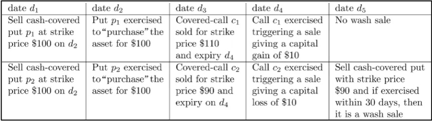
In a portfolio, individual capital gain values and individual capital loss values are usually distinct. Though rare, identical capital gains and capital losses are possible. Identical capital gains or losses are possible for portfolios built using options. We are ignoring option premiums. That is, asset purchases may be done via the exercise of cash-covered American-style put options. Also asset sales may be done via the exercise of American-style covered-call options. In these cases with options that become in-the-money, a portfolio manager has no control of the asset sales or purchases or timing of such trades. See Figure 1.

[image:11.595.122.553.510.632.2]

Most often, put or call option strike prices are at discrete increments. For example, many put and call equity options have strike prices in $5 or $10 increments. Suppose a portfolio is built only using the exercise of American-style options. Many asset gains and losses may be for identical amounts. Of course, this depends on the size of the underlying positions or the number of options written. Options with the same expiry on identically sized underlying assets may have very different values [10].

Figure 1. A potential wash sale with American-style options.Each row represents the same underlying asset type.

In such option-based portfolios assume uniform, independent, and random capital gains and capital losses. This may be modeled by the Littlewood-Offord Problem.

591 It is based directly on [4][6][41].

Definition 8 (Littlewood-Offord Problem) The integer Littlewood and Offord’s problem is given an integer multi-set V =

{

v v1, 2,,vn

}

where vi≥ ∀ ∈1, i

[ ]

n and

1 1 2 2

v n n

S =ξv +ξ v ++ξ v so each ξi is such that

[

]

[

]

1

1 1

2

i i

ξ = − = ξ = + =

  , for

[ ]

i∈ n , then what is maxx∈

[

Sv =x

]

?

Assuming equal probability of gains and losses and no drift [10]. Given an integer multi-set V =

{

v v1, 2,,vn

}

so vi≥ ∀ ∈1, i

[ ]

n . The multi-set V represents capital gains and capital losses. Capital gains and capital losses are all from sales. The iid Rademacher random variables ξi∈ + −

{

1, 1

}

determine if a vi is a capital gain or loss. All vi are positive since all the Rademacher variables have range

{

− +1, 1

}

, see also [5] and [40].

Over a tax year, the total capital gain or loss is

1 1 2 2 .

v n n

S =ξv +ξ v ++ξ v (12)

In an optimal solution of this version of the Littlewood-Offord problem, [5] showed the n-element multi-set V =

{

1,1,,1

}

has max_x

{

[

S_v x

]

}

O 1

n ∈

 

= _{=  }

 

  .

The next lemma’s proof follows immediately from the linearity of expectation given Rademacher random variables. See, for example, [39].

Lemma 3. Consider any integer multi-set V =

{

v v1, 2,,vn

}

where vi ≥ ∀ ∈1, i

[ ]

n and the random variable Sv =ξ1 1v +ξ2 2v ++ξn nv , where

[

]

[

]

1

1 1

2

i i

ξ = − = ξ = + =

  , for all i∈

[ ]

n , then 

[ ]

Sv =0.

For any Rademacher random variable ξi, it must be 

[ ]

ξi =0 and 2

1

i ξ   =  

 .

Since vi is constant

[ ]

2

2 2 2 2

i iv ivi i iv vi

ξ

σ =__ξ _−_ ξ = _{. Thus, a proof of the next}

theorem follows since the variance of a sum of independent random variables is the sum of the variances.

Theorem 4. Consider any non-negative integer vector v and the random variable

1 1 2 2

v n n

S =ξv +ξ v ++ξ v , where

[

1

]

[

1

]

1 2

i i

ξ = − = ξ = + =

  , for all i∈

[ ]

n , then

2 2 2 2

1 2

v n

S v v v

  = + + +

  

 and 2 2 2

1 2

v

S v v vn

σ = + ++ .

Thus, the lowest variance, 2

v

S

σ _{, for the integer Littlewood-Offord problem occurs} exactly when V =

{

1,1,,1

}

and V =n. Assuming the ξi,∀ ∈i

[ ]

n are all Rade-

macher random variables, then x∈

[

Sv =x

]

is maximized [6][40][41] as O

(

1 n

)

and σSv = n.

Theorem 4 implies the next corollary.

Corollary 1. Assume 1= =v1 v2==vn and Sv=ξ1 1v +ξ2 2v ++ξn nv where

[

]

[

]

1

1 1

2

i i

ξ = − = ξ = + =

  , for all i∈

[ ]

n , then the standard deviation of Sv is

v

S n

σ = _.

The generality of Theorem 4 asserts large variances too. Consider the set

{

0 1 1

}

2 , 2 , , 2n

V =  − , then by Theorem 4,

2 1 2 2

0

2 1

2 3

v

n n i S i

σ −

=

−

=

∑

= . This last equality

follows since the sum is a geometric series.

Definition 9 (Distinct sums of a set or multi-set V) Consider a set or multi-set

{

1, 2, , n

}

V = v v  v and let each element of the lists H₁= ξ ξˆ_1,1,ˆ_2,1,,ξˆ_n,1 and

2 ˆ1,2,ˆ2,2, ,ˆn,2

H = ξ ξ  ξ be fixed values from

{

− +1, 1

}

. The two sums of V,

,1 ˆ1,1 1 ˆ2,1 2 ˆ,1

v n n

s =ξ v +ξ v + + ξ v (13)

,2 ˆ1,2 1 ˆ2,2 2 ˆ,2 ,

v n n

s =ξ v +ξ v + + ξ v (14)

are distinct iff there is some ξˆi,1≠ξˆi,2, for i∈

[ ]

n .

Given any multi-set of positive integers V =

{

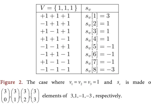
v v1, 2,,vn

}

, enumerate all 2 n _dis-

tinct sums as s_v

[ ]

1 ≥s_v

[ ]

2 ≥≥  s_v 2n , for example, see Figure 2. Given any set of

positive integers V =

{

v v1, 2,,vn

}

, where none of the 2

n _{distinct sums add to the}

same value gives s_v

[ ]

1 >s_v

[ ]

2 >>  s_v 2n .

An important observation by [5], is that for any fixed sum s the values s+vi and

i

s−v differ by 2vi. Next, this observation is used to show the set

{

}

0 1 1

2 , 2 , , 2n

V =  −

has no distinct sums that add to the same value.

In particular, take any distinct sums sv,1 and sv,2 with associated fixed values

{

}

,1

ˆ _{1, 1}

i

ξ ∈ − + _and ˆ_,2

{

_{1, 1}

}

i

ξ ∈ − + _{, respectively, for all} i∈

[ ]

n . Suppose, for the sake of

a contradiction, that sv,1=sv,2. Building on Erdös’ observation, the values sv,1 and

,2 v

s may be written as s_v,1=2n− −1 2m₁ where

1

1 1 2

i i I

m =

∑

_∈ − and I₁=

{

i:ξˆi_,1= −1

}

and likewise ,2 2 1 2 2 n

v

s = − − m where

2

1 2 2

i i I

m =

∑

_∈ − and I₂ =

{

i:ξˆ_i,2 = −1

}

, for all

[ ]

i∈ n . Finally, the uniqueness of binary-number representations means m1=m2 which in turn means ξˆi,1=ξˆi,2, for all i∈

[ ]

n . So, in fact, the sums sv,1 and sv,2 are equal, giving a contradiction.

Thus, the set

{

0 1 1

}

2 , 2 , , 2n

V =  − satisfies the antecedent of the next theorem.

Figure 2. The case where v1= = =v2 v3 1 and sv is made of

3 3 3 3

, , ,

0 1 2 3

               

        elements of 3,1, 1, 3− − , respectively.

Theorem 5. Among all sets of distinct positive integers where no two distinct sums add to the same value, the set

{

0 1 1

}

2 , 2 , , 2n

[image:13.595.242.500.485.664.2]

593

1 2 2 1

n

v n

s = +v v ++v = − .

Proof. Suppose, for the sake of a contradiction, that 1 2 2 1 n

v n

s = +v v ++v < − for

some set of distinct positive integers V =

{

v v1, 2,,vn

}

where no two distinct sums add to the same value.

Take the next enumeration of the 2n _{distinct sums,}

[ ]

₁

[ ]

_{2 2}n

v v v

s >s >>  s  , and

by our supposition, 2n− ≥2 s_v

[ ]

1 and s_v  ≥ − +_{ }2n 2n 2, so s_v

[ ]

1 −s_{v } 2n ≤2n+1−4.

Let

{

,1, ,2

}

{

[ ] [ ]

1 , 2 , , 2

}

n v v v v v

s s ⊆ s s  s  _{ } where sum sv,1 has the list of fixed values 1,1 2,1 ,1

ˆ _,ˆ _{, ,}ˆ

n

H = ξ ξ  ξ so that sv,1= v v1, 2,,vn ⋅H, where ⋅ is the vector dot pro- duct. Likewise, the sum sv,2 has the list of fixed values ξ ξˆ1,2,ˆ2,2,,ξˆn,2 .

The difference of any two distinct sums

s

v,1

−

s

v,2 must be even since any fixed

values ξˆi,1∈ − +

{

1, 1

}

and ξˆi,2∈ − +

{

1, 1

}

, for i∈

[ ]

n , are so that,

{

}

,1 ,2

ˆ ˆ _{0, 2, 2 ,}

i i

ξ −ξ ∈ − + ₍₁₅₎

giving

(

)

,1 ,2 ,1 ,2

1

ˆ ˆ

n

v v i i i

i

s s v ξ ξ

=

− =

∑

− ₍₁₆₎

which must be even.

Starting from sv

[ ]

1 and going to 2

n v

s  _{ } contains 2n−1 intervals. Since all

[ ]

v

s i , for 2n

i∈   , are different and their differences must be even so

[ ]

1 2n v v

s −  s  

spans at least

(

)

1

2 2n− =1 2n+ −2. That is, sv

[ ]

1 sv 2n 2n1 2

+

 

− _{ }≥ − _{. This gives a}

contradiction of the assumption

[ ]

1

1 2n 2n 4

v v

s −s  _{ }≤ + − , completing the proof.

Given a set of distinct positive integers V where V =n, Theorem 5 indicates that

[

]

{

}

1

max

2

x∈  Sv =x ≤ n . So in the case where all distinct sums of V add to different values, erasing a wash sale loss may have a very large impact. In particular, the multi-set

{

1,1, ,1

}

V =  has largest loss s_v  = −_{ }2n n, where Theorem 5 indicates

{

0 1 1

}

2 , 2 , , 2n

V =  − has the largest loss s_v  = − +_{ }2n 2n 1. In this case, when no distinct

sums add to the same value, let U =

{

2n−

(

2i−1 :

)

i∈   2n

}

giving

[

]

{

}

1

max

2

x U∈  Sv=x = n . Assuming wash sales occur with the same random and

uniform probability among all losses, the expected disallowed loss is 2n 1

n

− _{. This is}

because all losses are of the form

( )

1

2i−

− _{, for} i∈ +

[

n 1

]

, and by assumption these

losses all have the same probability of occurring.

Since 

[ ]

Sv =0 by Lemma 3, Littlewood-Offord results are useful for under-

standing likely values for Sv. That is, maxx∈ −{ }0

{



[

Sv=x

]

}

gives most likely capital gains or losses outside of the expected value 

[ ]

Sv =0. None of the sv values in

Figure 2 are 0, but if V has an even number of 1s, then the most common value is 0.

The following tail bound is given by [42] where 2 2 2

1, 2, , n 2 1 2 n

v v  v = v +v ++v ,

2₂

1 2 2 1

, , , e

n

t i i n i

v t v v v

ξ −

=

 _> _≤

 



∑

 

 (17)

2

2 2 2 2

1 2 e

t

v n

S t v v v −

 _{> + + +} _≤

 

  

2₂

e

v

t v S

S tσ −

 > ≤

 

 (19)

Since by Theorem 4, 2 2 2

1 2

v

S v v vn

σ = + ++ .

Suppose V =

{

1,1,,1

}

and V is odd. Since no sum of V is 0, there are

2 n capital gains and 2 n

capital losses. This means if Sv=tσ, then there are

2 2

n₊tσ

capital

gains and

2 2

n₋tσ

capital losses. Losses are necessary for wash sales. Therefore, the

bound 2₂

e

v

t v S

S tσ −

 > ≤

 

 gives the probability there are at least

2

v

S

tσ

more gains

than losses. That is, there are

2

v

S

tσ

fewer opportunities for wash sales.

Following Figure 2, given V =n then s_v

[ ]

1 =n is the case with zero capital losses.

Likewise, sv  = − 2n n is the case with zero capital gains. By Lemma 3, since 

[ ]

Sv =0 and sv

[ ]

1 + + sv  2n =0, thus

[ ]

2 2

n

v v

n s s  

− = _{+ +   . Also suppose a single wash} sale disallows a capital loss among all identical capital gains and losses. The single wash sale disallows a single capital loss giving the expected capital gain or loss:

[ ]

(

2 1

)

(

[ ]

3 1

)

(

2 1

)

.

2 1

n

v v v

n

s + + s + + + s  _{ }+

− 

(20)

The term sv

[ ]

1 is excluded since it has no losses, hence no wash sales.

The boy-girl ±30 birthday problem gives a necessary condition for wash sales of

substantially identical securities. Recall B30

(

252, ,g b

)

is the probability of at least one boy-girl ±30 birthday collision, so 1−B30

(

252, ,g b

)

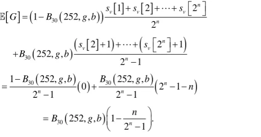
is the probability of no such birthday collision.

Given any number of boy-girl ±30 birthday collisions of the same security and

suppose these birthday collisions produce at most a single wash sale. In this case let G be a total taxable gain or loss where all gains and losses are the same. Suppose these gains and losses are all 1. This gives,

[ ]

(

30

(

)

)

[ ]

[ ]

1 2 2

1 252, ,

2

n

v v v

n

s s s

G B g b

 

+ _{+ +  }

= − 

 (21)

(

)

(

[ ]

)

(

)

30

2 1 2 1

252, , 2 1 n v v n s s

B g b

  + + + _{ }+ + −  (22)

(

_{) ( ) (}

)

₍

₎

30 30

1 252, , 252, ,

0 2 1

2 1 2 1

n

n n

B g b B g b

n

−

= + − −

− − (23)

(

)

30 252, , 1 .

2n 1

n

B g b  

= _ − _

−

  (24)

5. Conclusions and Further Directions

[image:15.595.189.553.64.356.2] [image:15.595.257.524.495.635.2]

595 Modeling and simulating taxes are important in both public policy settings as well as in practical tax planning. In public policy settings, conflicting fiscal and social policies make tax rules contentious. In tax planning, unexpected events may have serious consequences. Thus, reducing certain taxes to mathematical terms gives an unusual level of percision. Such percision can only benefit public policy and tax planning.

Acknowledgements

Thanks to Noga Alon and C.-F. Lee for insightful comments.

References

[1] von Mises, R. (1939) Über Aufteilungs-und Besetzungs-Wahrscheinlichkeiten. Revue de la Faculté des Sciences de l’Université d’Istanbul, 4, 145-163.

[2] Feller, W. (1968) An Introduction to Probability Theory and Its Applications. 3rd Edition, John Wiley, Hoboken.

[3] Cormen, T., Leiserson, C., Rivest, R. and Stein, C. (2001) Introduction to Algorithms. 2nd Edition, MIT Press, Cambridge.

[4] Littlewood, J. and Offord, A. (1943) On the Number of Real Roots of A random Algebraic Equation (III). Matematicheskii Sbornik, 12, 277-286.

[5] Erdös, P. (1945) On a Lemma of Littlewood and Offord. Bulletin of the AMS—American Mathematical Society, 51, 898-902. http://dx.doi.org/10.1090/S0002-9904-1945-08454-7

[6] Tao, T. and Vu, V. (2010) A Sharp Inverse Littlewood-Offord Theorem. Random Structures & Algorithms, 37, 525-539. http://dx.doi.org/10.1002/rsa.20327

[7] US Internal Revenue Service, Investment Income and Expenses (including Capital Gains and Losses) (2015) IRS Publication 550, Cat. No. 15093R for 2014 Tax Returns. See Pages 59+. https://www.irs.gov/pub/irs-pdf/p550.pdf

[8] FINRA Regulatory Notice 11-35, Effective 8-Aug-2011.

https://www.finra.org/sites/default/files/NoticeDocument/p124062.pdf

[9] Jensen, B. and Marekwica, M. (2011) Optimal Portfolio Choice with Wash Sale Constraints. Journal of Economic Dynamics and Control, 35, 1916-1937.

http://dx.doi.org/10.1016/j.jedc.2011.06.007

[10] Hull, J. (2015) Options, Futures, and other Derivatives. 9th Edition, Pearson, New York. [11] Constantinides, G.M. (1983) Capital Market Equilibrium with Personal Tax. Econometrica,

51, 611-636.

[12] Constantinides, G.M. (1984) Optimal Stock Trading with Personal Taxes: Implications for Prices and the Abnormal January Returns. Journal of Financial Economics, 13, 65-89.

http://dx.doi.org/10.1016/0304-405X(84)90032-1

[13] Dammon, R., Spatt, C. and Zhang, H. (2001) Optimal Consumption and Investment with Capital Gains Taxes. Review of Financial Studies, 14, 583-616.

http://dx.doi.org/10.1093/rfs/14.3.583

[14] Pat’s World Math Blog (2012).

http://pballew.blogspot.com/2011/01/who-created-birthday-problem-and-even.html [15] Ball, W. and Coxeter, H. (1987) Mathematical Recreations and Essays. 13th Edition, Dover,

New York, 45-46.

29. http://dx.doi.org/10.2307/2681879

[17] Abramson, M. and Moser, W. (1970) More Birthday Surprises. American Mathematical Monthly, 77, 856-858. http://dx.doi.org/10.2307/2317022

[18] Crilly, T. and Nandy, S. (1987) The Birthday Problem for Boys and Girls. The Mathematical Gazette, 71, 19-22. http://dx.doi.org/10.2307/3616281

[19] Pinkham, R. (1988) A Convenient Solution to the Birthday Problem for Girls and Boys. The Mathematical Gazette, 72, 129-130. http://dx.doi.org/10.2307/3618930

[20] Nishimura, K. and Sibuya, M. (1988) Occupancy with Two Types of Balls. Annals of the In-stitute of Statistical Mathematics, 40, 77-91. http://dx.doi.org/10.1007/BF00053956

[21] Galbarith, S. and Holmes, M. (2012) A Non-Uniform Birthday Problem with Applications to Discrete Logarithms. Discrete Applied Mathematics, 160, 1547-1560.

http://dx.doi.org/10.1016/j.dam.2012.02.019

[22] Selivanov, B. (1995) On the Waiting Time in a Scheme for the Random Allocation of Co-lored Particles. Discrete Mathematics and Applications, 5, 73-82.

http://dx.doi.org/10.1515/dma.1995.5.1.73

[23] Chatterjee, S., Diaconis, P. and Meckes, E. (2005) Exchangeable Pairs and Poisson Ap-proximation. Probability Surveys, 2, 64-106.

http://dx.doi.org/10.1214/154957805100000096

[24] Arratia, R., Goldstein, L. and Gordon, L. (1990) Poisson Approximation and the Chen- Stein Method. Statistical Science, 5, 403-424.

[25] DasGupta, A. (2005) The Matching, Birthday and the Strong Birthday Problem: A Con-temporary Review. Journal of Statistical Planning and Inference, 130, 377-389.

http://dx.doi.org/10.1016/j.jspi.2003.11.015

[26] Bradford, P., Perevalova, I., Smid, M. and Ward, C. (2006) Indicator Random Variables in Traffic Analysis and the Birthday Problem. 31st Annual IEEE Conference on Local Com-puter Networks (LCN 2006), Tampa, 14-16 November 2006, 1016-1023.

http://dx.doi.org/10.1109/lcn.2006.322217

[27] Stinson, D. (2005) Cryptography Theory and Practice. 3rd Edition, CRC Press, Boca Raton. [28] Song, R., Green, T., McKenna, M. and Glynn M. (2007) Using Occupancy Models to Esti-mate the Number of Duplicate Cases in a Data System without Unique Identifiers. Journal of Data Science, 5, 53-66.

[29] Diaconis, P. and Mosteller, F. (1989) Methods for Studying Coincidences. Journal of the American Statistical Association, 84, 853-861.

http://dx.doi.org/10.1080/01621459.1989.10478847

[30] DasGupta, A. (2004) Sequences, Patterns, and Coincidences.

http://citeseerx.ist.psu.edu/viewdoc/summary?doi=10.1.1.121.8367

[31] Apoport, A. (1998) Birthday Problems: A Search for Elementary Solutions. The Mathemat-ical Gazette, 82, 111-114. http://dx.doi.org/10.2307/3620175

[32] Flajolet, P., Gardy, D. and Thimonier, L. (1992) Birthday Paradox, Coupon Collectors, Caching Algorithms and Self-Organizing Search. Discrete Applied Mathematics, 39, 207- 229. http://dx.doi.org/10.1016/0166-218X(92)90177-C

[33] Motwani, R. and Raghavan, P. (1995) Randomized Algorithms. Cambridge University Press, Cambridge. http://dx.doi.org/10.1017/CBO9780511814075

[34] Mitzenmacher, M. and Upfal, E. (2005) Probability and Computing. Cambridge University Press, Cambridge. http://dx.doi.org/10.1017/CBO9780511813603

597 Probability. Springer, New York. http://dx.doi.org/10.1007/978-1-4612-4304-5

[36] Pinkham, R. (1985) 69.32 The Birthday Problem, Pairs and Triples. The Mathematical Ga-zette, 69, 279.http://dx.doi.org/10.2307/3617572

[37] Graham, R., Knuth, D. and Patashnik, O. (1994) Concrete Mathematics: A Foundation for Computer Science. Addison Wesley, Boston. http://dx.doi.org/10.2307/3617572

[38] Wendl, M. (2003) Collision Probability between Sets of Random Variables. Statistics & Probability Letters, 64, 249-254. http://dx.doi.org/10.1016/S0167-7152(03)00168-8

[39] Alon, N. and Spencer, J.H. (2008) The Probabilistic Method. 3rd Edition, Wiley, Hoboken.

http://dx.doi.org/10.1002/9780470277331

[40] Nguyen, H. and Vu, V. (2012) Small Ball Probability, Inverse Theorems, and Applications.

http://arxiv.org/abs/1301.0019

[41] Tao, T. and Vu, V. (2006) Additive Combinatorics. Cambridge University Press, Cam-bridge. http://dx.doi.org/10.1017/CBO9780511755149

[42] Montgomery-Smith, S. (1990) The Distribution of Rademacher Sums. Proceedings of the American Mathematical Society, 109, 517-522.

http://dx.doi.org/10.1090/S0002-9939-1990-1013975-0

Submit or recommend next manuscript to SCIRP and we will provide best service for you:

Accepting pre-submission inquiries through Email, Facebook, LinkedIn, Twitter, etc. A wide selection of journals (inclusive of 9 subjects, more than 200 journals)

Providing 24-hour high-quality service User-friendly online submission system Fair and swift peer-review system

Efficient typesetting and proofreading procedure

Display of the result of downloads and visits, as well as the number of cited articles Maximum dissemination of your research work

Submit your manuscript at: http://papersubmission.scirp.org/