A Monte Carlo Study for Swamy’s Estimate of Random Coefficient Panel Data Model

(1)

A Monte Carlo Study for Swamy’s

Estimate of Random Coefficient Panel

Data Model

Mousa, Amani and Youssef, Ahmed H. and Abonazel,

Mohamed R.

Department of Applied Statistics and Econometrics, Institute of

Statistical Studies and Research, Cairo University, Cairo, Egypt

11 April 2011

Online at

https://mpra.ub.uni-muenchen.de/49768/

(2)

A Monte Carlo Study for Swamy’s Estimate of Random

Coefficient Panel Data Model

Amani Mousa, Ahmed H. Youssef and Mohamed R. A

bonazel

Department of Applied Statistics and Econometrics, Institute of

Statistical Studies and Research, Cairo University, Cairo, Egypt.

particularly useful approach for analyzing pooled cross sectional and time series data is Swamy's random coefficient panel data (RCPD) model. This paper examines the performance of Swamy's estimators and tests associated with this model by using Monte Carlo simulation. The Monte Carlo study shed some light into how well the Swamy's estimate perform in small, medium, and large samples, in cases when the regression coefficients are fixed, random, and mixed. The Monte Carlo simulation results suggest that the Swamy's estimate perform well in small samples if the coefficients are random and but it does not when regression coefficients are fixed or mixed. But if the samples sizes are medium or large, the Swamy's estimate performs well when the regression coefficients are fixed, random, or mixed.

Key words: Random Coefficient Panel Data Model, Mixed RCPD Model, Panel Data, Monte Carlo Simulation, Pooling Cross Section and Time Series Data.

1. Introduction

Econometrics commonly uses “Time Series Data” describing a single entity. Another type of data called “Panel Data” which means any data base describing number of individuals across a sequence of time periods. To realize the potential value of the information contained in a panel data see Carlson (1978), Hsiao (1985, 2003), and Baltagi (2008). `

When the performance of one individual form the panel data is interest, separate regression can be estimated for each individual unit. Each relationship, on our model studied, is written as follows:

, ,..., 3 , 2 , 1

,..., 3 , 2 , 1 ,

1 0

T t

N i

x y_it _i _i _it _it

= = +

+

=β β ε

(1)

where i denotes cross-sections and t denotes time-periods. The ordinary least squares (OLS) estimators of β₀_i and β₁_i will be best linear unbiased estimators (BLUE) under the following assumptions:

(3)

A1: E(ε_i)=0

A2: E(

ε

_i

ε

_i′)=

σ

_i2I_T

A3: E(ε_iε′_j)=0, foralli≠ j.

These conditions are sufficient but not necessary for the optimality of the OLS estimator, see Rao and Mitra (1971). If assumption 2 is violated and disturbances are either serially correlated or heteroskedastic, generalize least squares (GLS) will provide relatively more efficient estimator than OLS, see Gendreau and Humphrey (1980). If assumption 3 is violated and contemporaneous correlation is present, we have what Zellner (1962) termed seemingly unrelated regression (SUR) equations. There is gain in efficiency by using SUR estimator rather than OLS, equation by equation estimator, see Zellner (1962, 1963).

Suppose that each regression coefficient in equation (1) is viewed as a random variable, that is, the coefficients β₀_i and β₁_i are viewed as invariant over time and varying from one unit to anther.

So, we are assuming that the individuals in our panel data are drown from a population with a common regression parameter,(β_j, j=0,1), which is fixed component, and a random component v_i which will allow the coefficients to differ from unit to unit, i.e.

A4: β_ji =β_j +v_ji, for i= 1,2,….,N, j=0,1.

Model (1) can be rewritten, under assumptions (1) to (4), as:

y_it =β₀_i +βG₁_i x_it +e_it, (2) where

it i it i

it

v

x

v

e

=

₀

+

₁

+

ε

, i =1,2,…,N, t=1,2,…T,

model (2) is called “Random Coefficient Panel Data” model examined by Swamy (1970, 1971, 1973, 1974), Kelejian and Stephan (1983), Hsiao and Pesaran (2004), and Murtazashvili and Wooldridge (2008).

Equation (2) can be written in matrix form as

e X

Y = β + , (3)

where

[

Y1Y2 YN

]

, Yi

[

y1iy2i yTi

]

, X

[

X1X2 XN

],

Y′= " ′= " ′= "

, ,

,

1 1 1

1 0 2

1

ε β

β

β = +

        = 

  

 

   

 

= e DV

x x x X

iT i i

i

#

(4)

, 0 0 0 0 0 0 2 1             = N X X X D " # % # # " "       =             = i i i N v v v v v v V 1 0 2 1 , # .

The following assumptions are added to the previous assumptions:

A5: The vector Vi are independently and identically distributed with E(vi)=0, and E(vivi′)=ψ,

i=1,2,…,N.

A6: The

ε

_it and v_i are independent for every i and j, so the variance-covariance matrix of e is , 0 0 0 0 0 0 ) ( 2 2 2 2 2 2 1 1 1 Ω σ ψ σ ψ σ ψ =               + ′ + ′ + ′ = ′ T N N N T T I X X I X X I X X e e E " # % # # " "

where zeros are T×T null matrices and

ψ

is the variance-covariance matrix of β_i as given in assumption (5). If assumptions (1) till (6) hold, then the GLS estimator of β is given by

Y X X

X 1 ₎ 1 1 (

ˆ ₌ _′_Ω− − _′_Ω−

β . (4)

Swamy (1970) showed that

[

]

_∑

[

]

∑

= − − − = − − ₊ _′       _′ + = N i i i i i N i i i

i X X X X

1 1 1 2 1 1 1 1 2 _ˆ ) ( ) (

ˆ _ψ _σ _ψ _σ _β

β

(5)

where βˆ is the OLS estimator of _i β_i. The GLS estimator cannot be used in practice, since ψ and σ_i2 are unknowns. Swamy (1971) suggested the following unbiased and consistent estimators

2 1 _{ˆ ˆ} ˆ_i _i _i

T K

σ = ε ε′

− , (6)

and

∑

= − ′ − − = N i i i i X X N

S

N 1

1 2

ˆ ˆ ( ) ,

1 1 1

ˆ σ

ψ _β ₍₇₎

where

∑ ∑

∑

= = = ′ − ′ = N i N i i i N i i i N S 1 1 1

ˆ ˆ ˆ.

1 ˆ

ˆ _β _β _β

β

(5)

Note that σˆ_i2 is the mean square error from the OLS regression of Y_i on X_i, and )

1 /(N−

Sβ is the sample variance-covariance matrix of βi. Substitute (6), (7), and (8) in (5),

we get the feasible generalized lest square (FGLS) estimator of βˆ as follows:

[

]

_∑

[

]

∑

= − − − = − − ₊ _′       ₊ _′ = N i i i i i N i i i

i X X X X

1 1 1 2 1 1 1 1 2 , ˆ ) ( ˆ ˆ ) ( ˆ ˆ

ˆ _ψ _σ _ψ _σ _β

β ₍₉₎

and the estimated variance-covariance matrix for the RCPD model is

[

ˆ ˆ ( )

]

,

, ) ( ˆ 1 1 1 1 2 1 1 − = − − − −       ₊ _′ = ′ =    

∑

N i i i

i X X

X X Var σ ψ Ω β (10)

Swamy (1973, 1974) showed that the estimator βˆ_i is consistent as both N and T →∞ and is asymptotically efficient as T →∞.

Because v_i is fixed for given i, we can test for random variation indirectly by testing whether or not the fixed coefficient vectors β_i are all equal. That is, we form the null hypothesis

β β β

β = = = _N =

H₀: ₁ ₂ " .

If different cross-sectional units have the same variance, σ_i2 =σ2, i=1,...,N, the conventional analysis of covariance test for homogeneity. If σ_i2 are assumed different, as postulated by Swamy (1970, 1971), we can apply the modified test statistic

∑

= − ′ ′ − = N i i i i i

i X X

F 1 2 * * ˆ ) ˆ ˆ ( ) ˆ ˆ ( σ β β β β _, (11) where       ′       ′ =

∑

= − = N i i i i N i i i i y X X X 1 2 1 1 2 * ˆ 1 ˆ 1 ˆ σ σ β .

Under H₀, (11) is asymptotically chi-square distributed, with K (N - 1) degrees of freedom, as T tends to infinity and N is fixed.

(6)

2. Simulation Design

A Monte Carlo simulation was conducted to study the behavior of certain estimators and tests in small, medium and large samples. The simulation was designed primarily to investigate estimation and hypothesis tests for the RCPD model discussed before. The settings of the model and results of the simulation study are discussed below.

The values of the independent variable

x

_it, were generated as independent normally distributed random variates with mean µ_X and standard deviation σ_X . The values of

x

_it were allowed to differ for each cross-sectional unit: However, once generated for all N cross-sectional units the values were held fixed over all Monte Carlo trials. The value of µ_X was set equal to zero and the value of σ_X was set equal to one. The disturbances, ε_it, were generated as independent normally distributed random variates, independent of the

x

_it values, with mean zero and standard deviation

σ

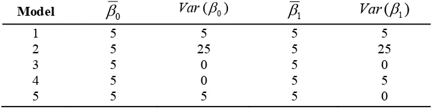
_ε . The disturbances were allowed to differ for each cross-sectional unit on a given Monte Carlo trial and were allowed to differ between trials. The standard deviation of the disturbances was set equal to either 1, 3, or 5 and held fixed for each cross-sectional unit. The values of N and T were chosen to be 10, 25, and 100 to represent small, medium and large samples for the number of individuals and the time dimension.

The parameters, β₀_i and β₁_i, were set at several different values to allow study of the estimators under conditions where the model was both properly and improperly specified. Also, test of hypothesis for randomness was examined to determine the observed level of significance and to obtain an idea of the power of the test. Five different combinations of β₀_i and β₁_i are used as given in Table (1). Note that a variance of zero simply means that the coefficient is fixed and equal over all cross-sectional units. These models will be estimated using Swamy's estimators in order to study the behavior of the coefficient mean estimator under misspecification of the model and to study the behavior of the tests for randomness of coefficients.

Table (1) Values of Coefficient Means and Variances Used in the Simulation

There are 45 experimental settings for the simulation, and 10,000 Monte Carlo trials were used for each settings. The results were recorded in Tables (2) through (6), with each table consisting of three panels, numbered I through III, for the different samples sizes (10, 25, and 100). And each panel from this panels corresponding to three settings of the disturbance standard deviation (1, 3, and 5). Each of the tables provides the results for a particular scheme of generation of the regression coefficients.

Model β₀ Var(β0) β₁ Var(β1) 1

2 3 4 5

5 5 5 5 5

5 25

0 0 5

5 5 5 5 5

5 25

[image:6.612.78.394.534.613.2]

(7)

3. Monte Carlo Results

Tables (2) through (6) are set up to show the following information:

The coefficient mean estimators (or the estimators of the fixed coefficients), βˆ₀ and βˆ₁, that are computed as in equation (9). The values shown in the first row of each panel of each table are the averages over all 10,000 Monte Carlo trials at a particular setting.

Table (2) Results of RCPD Estimation When β₀ ~ N (5, 5) and β₁ ~ N (5, 5)

σ

ε

N=T

1 3 5

0

β β₁ β₀ β₁ β₀ β₁

I. 10

βˆ 4.999 5.012 5.000 4.981 5.835 6.215

ψˆ 4.966 4.992 4.999 5.014 5.023 4.989

Bias of βˆ 0.001 -0.012 0.000 0.019 -0.835 -1.215

MSE of βˆ 0.508 0.515 0.592 0.627 1.404 2.209

% Negative Variance Estimates

0.0 0.0 0.1 0.2 1.0 1.9

%Rejections

0 :

2

0

σ

β

=

H

100.0 100.0 99.0 97.3 86.1 80.8

II. 25

βˆ 5.000 4.999 4.998 5.001 4.992 5.002

ψˆ 5.020 5.003 4.996 5.010 4.969 4.970

Bias of βˆ 0.000 0.001 0.002 -0.001 0.008 -0.002

MSE of βˆ 0.202 0.202 0.214 0.216 0.239 0.240

0.0 0.0 0.0 0.0 0.0 0.0

%Rejections

0 :

2

0

σ

β

=

H

100.0 100.0 100.0 100.0 100.0 100.0

III. 100

βˆ 4.999 4.998 4.999 5.000 5.002 5.000

ψˆ 5.000 4.996 4.999 4.999 5.002 5.007

Bias of βˆ 0.001 0.002 0.001 0.000 -0.002 0.000

MSE of βˆ 0.050 0.050 0.051 0.051 0.053 0.053

0.0 0.0 0.0 0.0 0.0 0.0

%Rejections

0 :

2

0

σ

β

=

[image:7.612.93.508.187.687.2]

(8)

Table (3) Results of RCPD Estimation When β₀ ~ N (5, 25) and β₁ ~ N (5, 25)

σ

ε

N=T

1 3 5

0

β β₁ β0 β1 β0 β1

I. 10

βˆ 4.997 5.026 5.008 4.998 5.015 4.998

ψˆ 24.816 24.943 24.972 25.089 25.062 24.986

Bias of βˆ 0.003 -0.026 -0.008 0.002 -0.015 0.002

MSE of βˆ 2.493 2.511 2.597 2.649 2.775 2.865

0.0 0.0 0.0 0.0 0.0 0.0

%Rejections

0 :

2

0

σ

β

=

H

100.0 100.0 100.0 100.0 99.8 99.7

II. 25

βˆ 5.000 4.998 4.998 5.001 4.981 5.001

ψˆ 25.101 25.011 24.978 25.071 24.866 24.886

Bias of βˆ 0.000 0.002 0.002 -0.001 0.019 -0.001

MSE of βˆ 1.006 1.002 1.014 1.018 1.036 1.038

0.0 0.0 0.0 0.0 0.0 0.0

%Rejections

0 :

2

0

σ

β

=

H

100.0 100.0 100.0 100.0 100.0 100.0

III. 100

βˆ 4.999 4.995 4.997 5.000 5.003 4.999

ψˆ 25.001 24.982 24.992 24.997 25.010 25.036

Bias of βˆ 0.001 0.005 0.003 0.000 -0.003 0.001

MSE of βˆ 0.250 0.250 0.251 0.251 0.253 0.253

0.0 0.0 0.0 0.0 0.0 0.0

%Rejections

0 :

2

0

σ

β

=

H

100.0 100.0 100.0 100.0 100.0 100.0

The estimated variance of each coefficient, (β ) ψˆ ^

=

k

Var , averaged over 10,000 trials, is shown in the second row. The estimates are computed as the diagonal elements in equation (7).

The bias value of the coefficient mean estimators, βˆ₀ and βˆ₁, are computed as

β β

βˆ₎ ˆ

( = −

bias where βˆ is a vector of coefficients mean estimators and β is a true vector of

[image:8.612.88.507.81.567.2]

(9)

Table (4) Results of RCPD Estimation When β0 = 5 and β1 = 5

σ

ε

N=T

1 3 5

0

β β₁ β0 β1 β0 β1

I. 10

βˆ 4.939 5.054 5.389 4.579 4.761 5.026

ψˆ 0.000 0.000 0.006 0.004 0.011 -0.017

Bias of βˆ 0.061 -0.054 -0.389 0.421 0.239 -0.026

MSE of βˆ 0.013 0.015 0.217 0.248 0.201 0.198

12.5 15.2 12.4 15.3 12.5 15.3

%Rejections

0 :

2

0

σ

β

=

H

25.0 25.0 25.7 24.9 25.4 25.4

II. 25

βˆ 5.006 5.008 4.991 4.994 5.033 5.017

ψˆ 0.000 0.000 -0.001 -0.002 -0.004 -0.002

Bias of βˆ -0.006 -0.008 0.009 0.006 -0.033 -0.017

MSE of βˆ 0.001 0.001 0.013 0.012 0.036 0.035

1.4 4.4 1.4 4.5 1.1 4.5

%Rejections

0 :

2

0

σ

β

=

H

12.3 12.4 12.1 11.7 12.5 12.3

III. 100

βˆ 5.000 5.000 5.000 5.000 5.000 5.000

ψˆ 0.000 0.000 0.000 0.000 0.000 0.000

Bias of βˆ 0.000 0.000 0.000 0.000 0.000 0.000

MSE of βˆ 0.000 0.000 0.001 0.001 0.002 0.002

0.0 0.0 0.0 0.0 0.0 0.0

%Rejections

0 :

2

0

σ

β

=

H

8.4 8.2 8.0 7.6 8.0 8.1

The Mean Square Error (MSE) of coefficient mean estimators that are computed as

2 ^

] ) ˆ ( [ ) ˆ ( ) ˆ

( k Var k bias k

MSE β = β + β where ( ˆ )

^ k

Var β is the estimated variance of the coefficient mean

[image:9.612.85.508.90.582.2]

(10)

Table (5) Results of RCPD Estimation When β₀ = 5 and β₁ ~ N (5, 5)

σ

ε

N=T

1 3 5

0

β β₁ β0 β1 β0 β1

I. 10

βˆ 5.058 4.966 4.298 4.593 4.893 4.970

ψˆ 0.000 5.019 0.002 4.973 0.000 5.046

Bias of βˆ -0.058 0.034 0.702 0.407 0.107 0.030

MSE of βˆ 0.014 0.517 0.339 0.700 0.211 0.799

10.5 0.0 11.1 0.6 11.0 2.6

%Rejections

0 :

2

0

σ

β

=

H

45.4 100.0 27.9 97.1 25.8 79.9

II. 25

βˆ 5.002 5.002 4.997 5.010 4.988 5.003

ψˆ 0.000 4.993 0.000 5.013 0.003 5.019

Bias of βˆ -0.002 -0.002 0.003 -0.010 0.012 -0.003

MSE of βˆ 0.001 0.201 0.013 0.216 0.037 0.241

0.8 0.0 0.8 0.0 0.9 0.0

%Rejections

0 :

2

0

σ

β

=

H

21.1 100.0 12.8 100.0 12.3 100.0

III. 100

βˆ 5.000 5.001 5.000 5.000 5.000 5.001

ψˆ 0.000 5.000 0.000 4.994 0.000 5.005

Bias of βˆ 0.000 -0.001 0.000 0.000 0.000 -0.001

MSE of βˆ 0.000 0.050 0.001 0.051 0.002 0.053

0.0 0.0 0.0 0.0 0.0 0.0

%Rejections

0 :

2

0

σ

β

=

H

14.7 100.0 8.3 100.0 7.8 100.0

It is possible to obtain negative estimates of the coefficient variances, 2

K

β

σ , when equation (7) is used to compute the variance-covariance matrix. The percentages of negative variance estimates shown in the row five of each panel.

The sixth row of each panel records the percentage of rejections of the null hypothesis

0 :

2

0 k

=

(11)

Table (6) Results of RCPD Estimation When β₀ ~ N (5, 5) and β₁ = 5

σ

ε

N=T

1 3 5

0

β β₁ β0 β1 β0 β1

I. 10

βˆ 4.987 4.829 4.845 4.953 3.388 4.690

ψˆ 5.018 0.000 5.000 -0.013 5.039 0.012

Bias of βˆ 0.013 0.171 0.155 0.047 1.612 0.310

MSE of βˆ 0.511 0.034 0.613 0.135 3.078 0.359

0.0 14.4 0.3 14.1 1.4 13.9

%Rejections

0 :

2

0

σ

β

=

H

100.0 48.6 98.8 27.6 86.2 26.7

II. 25

βˆ 5.001 4.976 5.005 4.993 4.989 4.989

ψˆ 4.993 0.000 5.016 0.002 5.019 0.003

Bias of βˆ -0.001 0.024 -0.005 0.007 0.011 0.011

MSE of βˆ 0.201 0.002 0.215 0.013 0.240 0.032

0.0 4.1 0.0 4.3 0.0 4.4

%Rejections

0 :

2

0

σ

β

=

H

100.0 20.6 100.0 13.2 100.0 12.8

III. 100

βˆ 5.001 5.000 5.000 5.000 5.001 5.000

ψˆ 5.001 0.000 4.997 0.000 5.005 -0.001

Bias of βˆ -0.001 0.000 0.000 0.000 -0.001 0.000

MSE of βˆ 0.050 0.000 0.051 0.001 0.053 0.002

0.0 0.0 0.0 0.0 0.0 0.0

%Rejections

0 :

2

0

σ

β

=

H

100.0 14.3 100.0 8.4 100.0 8.0

As a guide to interpreting the tables, let us consider Table (2) as an example. When 1

=

σε and N=T=10 (small samples), the averages mean and variance for β₀ over all 10,000 Mote Carlo trials are 4.999 and 4.966 respectively. Note that the true coefficients values for mean and variance are 5 and 5, and the values of bias and MSE for βˆ₀ are 0.001 and 0.508. And the averages mean and variance for β₁ are 5.012 and 4.992 respectively. While the true coefficients values for mean and variance are 5 and 5. While the percentage of negative variance estimates for βˆ₀ and βˆ₁ is zero. Note that this percentage should be zero. And the

[image:11.612.84.509.77.570.2]

(12)

that the randomness test is performing as designed even in small samples. As the variation in the disturbances increase, from σε =1 to σε =3, the estimators get worst. Increasing both the number of individuals and the time series data will make the estimators better.

4. Concluding Remarks

From Tables (2) till (6), several observations concerning the RCPD estimators and the test statistics for the randomness test can be made:

1- The Swamy's estimators performs well when the coefficients are random, even though the samples are small (T=10). The biases, (true coefficient – estimated coefficient), of the Swamy's estimators of β_i and ψ decrease when the time series observations and the number individual units getting large. From Tables (2) and (3), the bias and MSE are doing better in small and large variation of the parameters. In general, the Swamy's estimate perform best when both coefficients are random.

2- When the coefficients are random, a small number of negative variance estimates occurs for the small sample size, the negative variance estimates does not appear in medium and large samples.

3- When both coefficients are fixed, Table (4), and the sample size is small, the RCPD model is inappropriate and a large number of negative variance estimates occurs as suggested in Dielman (1980). Thus, the appearance of negative variance estimates would suggest the possibility that the coefficient be treated as fixed.

4- When both coefficients are fixed and the samples sizes are medium or large, the RCPD model is appropriate and the negative variance estimates will not appear.

5- When one of the coefficients is fixed and the sample size is small, the Swamy's estimators will not perform as well as might be expected. The appearance of negative variance estimates, in Tables (5) and (6), would suggest misspecification occurrence in the assumptions. But if the samples sizes are medium or large, the Swamy's estimators perform well.

6- The test for randomness performs well overall. The best produces a high percentage of

rejections of the hypothesis

H

₀

:

σ

2βk

=

0

is when the coefficients are random and a

low percentage when the null hypothesis is true.

7- As the variation in the disturbances increases (relative to the variation due to the explanatory variable), the performance of the Swamy's estimators deteriorates. This is also true for the power of the test for significance of the coefficient means.

(13)

The Monte Carlo simulation results suggest that the Swamy’s estimators perform well in small samples if the coefficients are random and but it does not in fixed or Mixed RCPD models. But if the samples sizes are medium or large, the Swamy’s estimators performs well for the three models. Finally, some caution must be taken before using the Swamy’s estimators, and pretesting procedures of the randomness of the coefficients must be made. This simulation has been limited in scope, as all simulations must be. Hopefully it will shed some light on performance of Swamy’s estimators in panel data.

References

1. Baltagi, B. (2008), Econometric Analysis of Panel Data. 4th ed., John Wiley and Sons Ltd. 2. Carlson, R. (1978), “Seemingly Unrelated Regression and the Demand for Automobiles of

Different Sizes.”, Journal of Business, Vol. 51, pp. 243-262.

3. Dielman, T. E. (1980), Pooled Data for Financial Markets (Research for Business Decision Series). Ann Arbor: UMI Research Press.

4. Gendreau, B. and Humphrey, D. (1980), “Feedback Effects in the Market Regulation of Bank Leverage: A Time-Series and Cross-Section Analysis.”, Review of economic Statistics, Vol. 62, pp. 276-280.

5. Hsiao, C. (1985), “Benefits and Limitations of Panel Data.”, Econometric Review, Vol. 4, pp. 121-174.

6. Hsiao, C. (2003), Analysis of Panel Data. 2th ed., Cambridge: Cambridge University Press.

7. Hsiao, C. and Pesaran, M. H. (2004), “Random Coefficient Panel Data Models.”, IEPR Working Paper 04.2, University of Southern California.

8. Kelejian, H. H. and Stephan, S. W. (1983), “Inference in Random Coefficient Panel Data Models: A Correction and Clarification of the Literature.”, International Economic Review, Vol. 24, pp. 249-254.

9. Murtazashvili, I. and Wooldridge, J. M. (2008), “Fixed Effects Instrumental Variables Estimation in Correlated Random Coefficient Panel Data Models.”, Journal of Econometrics, Vol. 142, pp. 539-552.

10.Rao, C. R. and Mitra, S. (1971), Generalized Inverse of Matrices and Its Applications.John Wiley and Sons Ltd.

11.Swamy, P. (1970), “Efficient Inference in a Random Coefficient Regression Model.”, Econometrica, Vol. 38, pp. 311-323.

12.Swamy, P. (1971), Statistical Inference in Random Coefficient Regression Models. New York: Springer-Verlag.

13.Swamy, P. (1973), “Criteria, Constraints, and Multicollinearity in Random Coefficient Regression Model.”, Annals of Economic and Social Measurement, Vol. 2, pp. 429-450. 14.Swamy, P. (1974), Linear Models with Random Coefficients. in Frontiers in Econometrics

(Ed. P. Zarembka).”, New York: Academic Press, Inc., pp. 143-168.

15.Zellner, A. (1962), “An Efficient Method of Estimating Seemingly Unrelated Regressions and Tests of Aggregation Bias.”, J.A.S.A., Vol. 57, pp. 348-368.