http://www.scirp.org/journal/jmp ISSN Online: 2153-120X ISSN Print: 2153-1196
Spring Theory as an Approach to the
Unification of Fields
Ling Man Tsang
Fisica Laboratorio, TIS, Macau University of Science and Technology, Macau, China
Abstract
The cosmological constant is necessary to be retained in Einstein’s field equations with value depending on the mass of the source. An overview of the spring theory in astrophysics and cosmology is included in this paper. In short range force, the two interacting particles are point-like vertices connected by a bosonic spring. We also suspect that electron may contain negative sterile neutrino. The self energy of a point charge is not infinite so that renormalisation is not necessary.
Keywords
Cosmological Constant, Dark Matter, Classical Electrostatics, Short Range Interaction
1. Introduction
Astrophysical standard model has confirmed to accept the cosmological constant in re-lating to dark energy—undetectable particles same as dark matter. The matter distribu-tion inside the universe is roughly dark fluid 95 percent and normal matter 5 percent. Different notions such as dark energy, dark matter, aether, pure space and others are of the same entity. They are different manifestations of the same dark fluid aether, just like the extension and compression of a spring [1][2]. The famous Michelson-Morley ex-periments provide no proofs to decline the existence of aether; moreover, the basic as-sumptions of these experiments are wrong [3][4]. The theory in this paper is in fact a three dimensional treatment of the de-Sitter Schwarzschild solution. Simply speaking, a spring term is added into Newton’s gravitation. With such a model, we can derive easily the Hubble’s law, explain the missing mass in the rotation curve of galaxies, and depict the short range interaction in which the two point-like vertices are connected by a bo-sonic spring. Spring theory is based on two resources; the theoretical Yang’s pure space and the results of the Pound-Rebka experiments on the photonic frequency changes How to cite this paper: Tsang, L.M. (2016)
Spring Theory as an Approach to the Unifi-cation of Fields. Journal of Modern Physics, 7, 2219-2230.
http://dx.doi.org/10.4236/jmp.2016.715192
Received: September 16, 2016 Accepted: November 27, 2016 Published: November 30, 2016
Copyright © 2016 by author and Scientific Research Publishing Inc. This work is licensed under the Creative Commons Attribution International License (CC BY 4.0).
http://creativecommons.org/licenses/by/4.0/
along a vertical path.
1.1. Yang’s Pure Space [5]
; ;
Rµν λ=Rµλ ν (1)
Or, after contraction of µ and ν
; ; .
u
Rλ =Rλ µ (2)
Properties of these equations had been studied by various authors [6][7][8]. Pavelle [6] pointed out that Yang’s pure space is non-physical unless the cosmological constant remains in Einstein’s field equations which was later verified by Mielke [8]. We begin from the second Bianchi Identity
; ; ; 0.
n n n
ikl m ilm k imk l
R +R +R =
(3)
For n=l, we have
; ; ; 0
n ik m im k i mk n
R −R −R = (4)
Operating ik
g on above, we have
; ; ; 0
k n
m m k m n
R −R −R = (5)
; ;
1 2
k
m k m
R = R (6)
Comparing with Equation (2), R is a constant. Now the Einstein’s field equations with the cosmological constant can be written as
1
0 2
Rµν − g Rµν +gµνΛ = (7)
We obtain in the 4-dimensional case
Rµν =gµνΛ (8)
4
R= Λ (9)
indicating that Einstein’s case is a special solution of Yang’s pure space where the cova-riant derivative of the Ricci tensor in Einstein’s case is zero but not in Yang’s case.
Hence, the cosmological constant needs to be retained but to be re-named as spring con-stant since it behaves like a harmonic oscillator as we can see later. In a 3-dimensional space, a spring term is added into Newton’s law of gravity:
(
)
2 replaces Λ
GM
kr a k
r ± = (10)
where k is the spring constant of the source while Λ is assigned as the spring constant of the universe which also known as the cosmological constant. Throughout this paper, only 3-dimensional springs are to be considered.
1.2. The Pound-Rebka Experiments
pho-tons under the earth’s gravity. The Jefferson Physical Laboratory at Harvard used a 57Fe
source placed at a height of 22.6 m above the detector.
Data were obtained when the gamma ray dropped onto the detector:
11
3.5 10 eV
h∆ =ν × − (11)
height dropped 22.6 m
∆ = (12)
0 0 source energy 14.4 keV
E =hν = (13)
2
2
0
9.67 m s
c
a ν
ν ∆
= =
∆ (14)
which is only true at Harvard, or likewise, the state of Massachusetts. In 1965 Pound and Snider refined the apparatus so that the energy shifts on the upward and downward path gave the measured difference of
(
)
( )
15down up 4.905 10
E E
E E
−
∆ −∆ = × (15)
Since the first term of Equation (15) is known, the second term will immediately yield the deceleration of 2
9.85 m s . Taking
the earth’s rotation 7.3 10ω= × −5 sec (16)
the earth’s radius 6 0
6.4 10 mr = ×
(17)
the earth’s mass 24
6 10 kg
= ×
(18)
42
θ = (19)
being the latitude of Massachusetts where Pound and Rebka performed their experi-ments at Harvard. Upon substituting the acceleration 9.67 m s2 and deceleration
2
9.85 m s into Equation (10), we obtain the following two equations
2 2 2
0 0
2 0
cos 9.67 m s
GM
r kr
r −ω θ− = (20)
2 2 2
0 0
2 0
cos 9.85 m s
GM
r kr
r −ω θ+ = (21)
Thus, the spring constant of the earth k=1.21 10× −8 s2 which, as expected, is
dif-ferent from the cosmological constant. The spring term is so-called because it behaves like an harmonic oscillator.
2. An Overview of the Spring Theory in Astronomy
and Astrophysics
2.1. Spring of the Earth
From Equation (10), there exists a point or a spherical shell at a distance of r=32000 km away from earth where the spring and the earth gravity cancel out each other to give
0
a= :
(
)
2 32000 km
GM
kr a r
(
)
2 0 32000 km
GM
kr r
r − = = (23)
(
)
2 32000 km
GM a r
r = > (24)
The last equation shows that the spring breaks at the distance of 32,000 km away from us. Equation (10) gives a clear picture of the fifth force different from the Yukawa type [9]-[15]. However, we have pointed out that the Yukawa type of fifth force is non-logical at a=0 and cannot predict Equations ((22), (23) and (24)).
2.2. The Spring of the Moon
The almost vacuum lunar surface provides a frictionless condition for a free falling test to verify the existence of the fifth force as well as to obtain the spring of the moon. The total time travelled by a free falling object through a height H can simply be found as
1 2
2H T
g kH
= −
(25) where g=1.627 m s2 is the moon’s gravity.
If fifth force does exist, the total time T must take longer than the classical one with-out the spring term [16].
2.3. The Spring of the Sun
The Binet Equation (53) yields the solution [17]
2 2 4
2 2 2 3 3
1
cos 1 2
GM G M kh
u kD
r h h c φ G M
= = + − − (26)
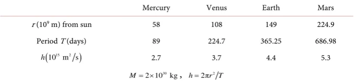
[image:4.595.193.556.487.570.2]where D is a constant. Setting the cosine part to zero, the spring of the sun is
Table 1. Orbital details of the inner planets.
Mercury Venus Earth Mars r (109 m) from sun 58 108 149 224.9
Period T (days) 89 224.7 365.25 686.98
(
15 2)
10 m s
h 2.7 3.7 4.4 5.3
30
2 10 kg
M= × , 2
2π
h= r T
Table 2. Comparison of different k (/sec2) values.
Jetzer [18] Cardona [19] Iorio [20] Adkins [21] Tsang
Mercury 10−24 - 10−24 - 10−14
Venus 10−22 - 10−22 - 10−15
Earth 10−25 - 10−25 - 10−16
Mars 10−25 - 10−25 - 10−16
[image:4.595.189.556.605.705.2]3 3
4 2
1
G M GM k
r
h h
= −
(27) Table 1 can be found in many astronomy textbooks. From Table 2, we can see that the average value of k is higher than those from various authors.
There are two main reasons of difficulty in determining the value of the sun’s k: • the value of the two terms inside the bracket of Equation (27) is so close to each other. • planetary interaction has not been taking into account.
However, the spring term of Equation (26) contributes insignificantly in the perihe-lion shift of planetary motion as well as the bending of light while grazing the sun.
2.4. The Cosmological Constant of the Universe
There are 3 main parameters in any cosmological model, namely the cosmological con-stant, the Hubble constant and the matter density [22]. In such a large scale structure, 3 dimensional space is sufficient to depict the universe instead of general relativity [23], Milne [24] and McCrea [25] used Newtonian mechanics to derive the cosmological eq-uations while Harrison used the first law of thermodynamics and eqeq-uations of hydro-dynamics [26].
In the beginning, all matters were compressed into a high density lump of universe followed by a release in such a way that all matters were sprung out by the spring(s) as governed by the equation
3
2
4 π d 3
d
r G
v
r a v
r r
ρ
Λ − = =
(28)
which is the same approach as Konuschko [27] except the cosmological term was not considered in his paper. Now,
35 2
10− s
Λ (29)
27 3
present density of our universe ρ10− kg m (30)
11 3 2
10 m sec kg
G −
(31)
26
present radius of our universe R4 10 m×
(32)
Equation (28) can be reduced to, upon integration:
(
)
1 12 2
v= Λ −Gρ r= Λ r
(33)
which is just the Hubble’s law having the Hubble constant 17.5
10 s
H − in agreement
with many literatures [28] where they related Λ to ACDM model. From the above data, total mass of the universe is 51
10 kg
M . Hence, the universe stops to accelerate
when
2 0
GM r
r
Λ − = (34)
or 26
10 m
at the outer rim of the universe exceeds the speed of light, i.e. ~108.5 m/s. Superluminal
recession of galaxies is acceptable by some cosmologists [29][30].
2.5. The Missing Mass in the Rotation Curve of Galaxies
It is already known that the cosmological constant is the answer of dark matter [31], or more precisely, variable cosmological constant [32]. This is explicitly referring to the spring constant of the galaxy, but awaiting to be spelt out. Again, in such a large scale of structure, only approximate estimation can be achieved with the following assumptions: • aberrations in the observed velocity and distance are unavoidable [33][34].
• the radius R of the cluster and the velocity can be estimated from the rotation curve.
• • 19
1 kpc= ×3 10 m.
In the quantum version of the virial theorem, the average value of the operator T in energy eigenstates in one dimension is given by
1 2
V
n T n n x n
x ∂ =
∂ (35) where T is kinetic energy and V is potential energy. Since the angular velocity of the galaxies is very small: ω10−15 s, the viral theorem holds.
We have studied the rotation curves of galaxies in Figure 1 and Figure 2 with the help of the virial theorem.
( )
2 GM r 2
v kr
r
= +
(36)
Nearly all these rotation curves yield the same (for detail see [17])
2
41
10 kg
v R M
G
=
(37)
31 2
10 sec
k= − (38)
It is clear that each mass has only one unique spring constant assigned to it. Strictly speaking. a flat curve means that the mass is still decreasing depending on 2 2
v −kr in the virial theorem but good approximation of k can be obtained even though v remains constant over several kpc’s. We take two other papers as a comparison. Firstly, we con-sider Gessner’s paper [37] who used general relativity to investigate 6 NGC’s, found the
mass of galaxies 41
1.8 10
M = × to 8 10 kg× 41 and the spring constant 31
10
k= − to
33 2
10− s . The results matched our work. The second paper belonged to an Indian team led by B. Aryal [38]. They also used general relativity to investigate 15 NGC’s, found
0.13
M = to 7.6 10 kg× 40 , and the spring constant k= −2.7 to − ×9 10−31 s2 which
is negative. Based on the information in their paper including the value of M, we used the virial theorem to obtain a positive value of k10−31 s2. Once again, in large scale
structure, 3 dimension is sufficient to depict astrophysical phenomena.
3. The Electric Field
Figure 1. NGC 4594, 2590, 1620 and 7664 [35].
Figure 2. Circular speed versus radius of our galaxy: curve D for le vancouleurs and Pence. B for Bathcall and Soneira [36].
2
W =aE (39)
Since a charge is always accompanied by its electromagnetic mass δm, the total mass of a charge particle is M = mechanical mass + electromagnetic mass δm. The above two masses are non-separable from each other. The relationship of the charge and field density is assumed as
2
4π e
E ρ aE
∇ ⋅ = = (40)
which seems to be reasonable to say the energy density of the source is proportional to the energy density of its surrounding field. Upon integration
1
2 1
A B
E
r r
−
= +
(41) A and B are constants. Integrating over the whole space, and set A = charge q, the total energy
2 2
2
total 0 2
1
1 d 2
q B
W r mc
r
r δ
−
∞
= + =
[image:7.595.253.498.104.420.2]which is just the Gauss Law except the right hand side of of Equation (42) is not me in
the case of electron. Thus 2 2
2
q B
mc δ
≈ . The field intensity becomes
1 2
2 1 2
2
q q
E
r
δ
mc r−
= +
(43) The potential can be written as
(
)
3
13
2 2 long range, 10 m
4
q q
r mc r φ
δ
−
= − + > (44)
(
)
ln 1 short range
A B
B r
= +
(45)
where A and B need to be determined in short range since coupling is involved. Ob-viously, for δ =m 0, E= 0, showing that the electromagnetic mass always accompa-nies with the charge. We can use Bohr’s atomic model to find δm. The three key equa-tions including the force, energy and the conservation of angular momentum are, re-spectively
2 2 4
2 2 3
2
mv e e
r =r − δmc r + (46)
2 2 4
2 2
13.6 eV
2 4
mv e e
E
r δmc r
= − = − + + (47)
and
mvr= (48)
Among the 4 pairs solution after solving the above, the most logical pair is
11
5.29 10 m
r= × − , 33
2.2 10 kg
m
δ = − × − . There were queries about the internal
struc-ture of electron in the last century [39]. Bonnor even raised the question “Does electron contain negative mass?” [40]. As already known [41] that the electron mass
(
0.51 MeV c2)
is totally electromagnetic but the radius of the electron is not 215 2
e
2.8 10 m
e R
m c
−
×
(49)
Instead, through the electron-positron scattering, the upper limit of 18
2 10 m
R × − implies that there is a complex internal structure. The Bohr model provides rooms for the electromagnetic mass but not the spring term. Most probably the spring of the pro-ton at the nucleus breaks off before reaching the orbiting electron. It is yet unknown of how much energy is required to bring this negative mass into the physical world. Another explanation of the negative energy particle is to connect it with anti-particles, or most likely the anti-electron neutrinos having positive energy. The expectation value of the additional term in Equation (47) will produce a perturbation term of
4 2 2 1 4 nlm e
E nlm nlm
mc r
δ
∆ = (50)
spectrum.
4. The Gravitational Field
As both the Coulomb and Newton’s inverse square law are analogous to one another, the gravitational field from Equation (42) becomes
2 2
2 2
0
1
1 d 2
GM B
r Mc
r r
−
∞
+ =
∫
(51)where 2 2
GM B
c
= . The field intensity Equation (43) in gravitation becomes
(
)
2 2
2 2 3 long range
2
GM G M a
r − c r = (52)
Including the spring term, the new Binet equation can be written as
2 2 2
2 2 2 2 2 3
d
d 2
u GM G M u k
u
h c h h u
φ + = − +
(53)
To solve for the above Equation (53), we followed the same procedures as in [42] and [43] to get Equation (26). Comparing the tests with general relativity, the spring term contributes insignificantly in the bending of light while grazing the sun whereas the pe-rihelion shift of a planet gives
2 2
2 2
2π 1 4
G M h c
δφ
= − (54)
5. Spring in the Short Range Interaction
Figure 3 shows the quarkonium potential energy which can be governed by the fol-lowing 3 equations:
a) Cornell potential
( )
a V r brr
= + (55)
[image:9.595.262.483.519.687.2]where a= −0.059 GeV fm⋅ , b=1.16 GeV fm.
b) Natural log potential
( )
ln( )
V r =a br (56)
where a=0.75 GeV, b=4.06 fm.
c) Spring theory (Equation (45) + spring term)
( )
ln 1 bV r a C
r
= + +
(57) where a and b can be estimated roughly from the graph. However, the constant C is in fact the energy of the spring or rather say, the energy of the confined quarkonia. It fol-lows that
2 1 2
2
q q
m c = m kr =C (58)
There are many combinations of a and b in Equation (57). For instance, for charmo-nium, C=3.3 GeV,a= −1.15 GeV and b=4.36 fm. For bottomonium,
9.3 GeV
C= , a= −2.8 GeV and b=10.9 fm. The above values are not accurate based on trial and error. However, Equation (57) is the general form for short range in-teractions. The Cornell potential had been applied in the s-wave with radial quantum number n=1, 2, 3, 4 of heavy quarkonia. By solving the Schrödinger equation, nu-merous energy eigenvalues are listed [45]. In fact, tracing back to 1981 [46], or even earlier, the Cornell potential was recommended as the unified potential for quarkonia, mesons and baryons. We hereby encourage particle physicists to use spring theory.
6. Discussions
Revisiting the equations from (40) to (45), we come to something interesting: • total field energy of a charge particle with radius R
(
)
12 4π 2 d constant constant 1 R
B
E r r
R
−
∞
∼ = + +
∫
(59)• total self energy of a charge with radius R
(
)
12 2
0 4π d constant 1
R B
E r r
R
−
= +
∫
(60)
For R = 0, none of the above tends to infinity. In a book written by Sapogin [47], it was mentioned that the classical theory of electromagnetism was fundamentally wrong. The electric field at the centre is zero because E is a vector. Feyman pointed out that Coulomb’s inverse square law fails at very short distance (see Feyman Lectures on Physics volume 2 chapter 5.8). Hence, renormalisation is not necessary. Perhaps short range Maxwell’s equations can be furtherly elaborated towards a new branch of elec-tromagnetism [48].
References
[1] Zhao, H. (2007) The Astrophysical Journal Letters, 67, L1-L4.
[2] Tsang, L.M. (2012) Applied Physics Research, 4, 229-232. [3] Sandhu, G.S. (2016) Applied Physics Research, 8, 45-57.
https://doi.org/10.5539/apr.v8n3p45
[4] Apsden, H. (1969) Physics without Einstein. Sabberton Publication, University of Sou-thampton, SouSou-thampton, 36, 59.
[5] Yang, C.N. (1974) Physical Review Letters, 33, 445-447.
https://doi.org/10.1103/PhysRevLett.33.445
[6] Pavelle, R. (1974) Physical Review Letters, 33, 1461-1463.
https://doi.org/10.1103/PhysRevLett.33.1461
[7] Guilfoyle, B.S. and Nohan, B.C. (1998) General Relativity and Gravitation, 30, 473-495.
https://doi.org/10.1023/A:1018815027071
[8] Mielke, E.W. and Maggiolo, A.A.R. (2005) General Relativity and Gravitation, 37, 997- 1007. https://doi.org/10.1007/s10714-005-0083-2
[9] Burgess, C.P. and Cloutier, J. (1988) Physical Review D, 3, 2944-2964.
https://doi.org/10.1103/PhysRevD.38.2944
[10] Fischbach, E. and Talnadge, C. (1992) Nature, 356, 207-215. [11] Sereno, M. and Jetzer, P. (2006) MNRAS, 371, 626-632.
https://doi.org/10.1111/j.1365-2966.2006.10670.x
[12] Iorio, L. (2007) Planetary and Space Science, 55, 1290-1298.
https://doi.org/10.1016/j.pss.2007.04.001
[13] Haranus, I. and Ragos, O. (2011) Astrophysics and Space Science, 331, 115-119.
https://doi.org/10.1007/s10509-010-0440-9
[14] Kolosnisyn, N.I. and Melnikov, V.N. (2004) General Relativity and Gravitation, 36, 1619- 1624. https://doi.org/10.1023/B:GERG.0000032154.73097.5b
[15] Lucchesi, D.M. (2003) Physics Letters A, 318, 234-240.
https://doi.org/10.1016/j.physleta.2003.07.015
[16] Tsang, L.M. (2012) New Astronomy, 17, 18-21.
https://doi.org/10.1016/j.newast.2011.05.004
[17] Tsang, L.M. (2013) Journal of Modern Physics, 9, 1205-1212.
https://doi.org/10.4236/jmp.2013.49164
[18] Jetzer, P. and Sereno, M. (2006) Physical Review D, 73, Article ID: 044015.
https://doi.org/10.1103/PhysRevD.73.044015
[19] Cardona, J.F. and Tejeiro, J.M. (1998) The Astronomical Journal, 493, 52-53.
https://doi.org/10.1086/305125
[20] Iorio, L. (2006) International Journal of Modern Physics D, 15, 473-476.
https://doi.org/10.1142/S021827180600819X
[21] Adkins, G.S. and Mc Donnell, J. (2007) Physical Review D, 75, Article ID: 082001.
https://doi.org/10.1103/PhysRevD.75.082001
[22] Bertin, G. (2014) Dynamics of Galaxies. 2nd Edition, Chapter 4, Cambridge University Press, Cambridge. https://doi.org/10.1017/CBO9780511731990
[23] Perlmutter, S. and Schmidt, B.R. (2003)Measuring Cosmology with Supernovae. In: Wei-ler, K., Ed., Supernovae & Gamma Ray Bursts, Springer, Berlin, 195-217.
https://doi.org/10.1007/3-540-45863-8_11
[24] Milne, E.A. (1934) Quarterly Journal of Mathematics, 5, 64-72.
[25] McCrea, W.H. and Milne, E.A. (1934) Quarterly Journal of Mathematics, 5, 73-80.
https://doi.org/10.1093/qmath/os-5.1.73
[26] Harrison, E.R. (1965) Annals of Physics, 37, 437-446.
https://doi.org/10.1016/0003-4916(65)90249-6
[27] Konuschko, V. (2012) Journal of Modern Physics, 3, 1819-1829.
https://doi.org/10.4236/jmp.2012.311227
[28] Freedman, W.L. and Madore, B.E. (2010) Annual Review of Astronomy and Astrophysics, 48, 673-710. https://doi.org/10.1146/annurev-astro-082708-101829
[29] Davis, T.M. and Lineweaver, C.H. (2004) Astronomical Society of Australia, 21, 97-109.
https://doi.org/10.1071/AS03040
[30] Kiang, T. (2003) Chinese Journal of Astronomy and Astrophysics, 27, 247-251. [31] Peebles, P.J.E. and Ratra, B. (2003) Reviews of Modern Physics, 75, 559-606.
https://doi.org/10.1103/RevModPhys.75.559
[32] Mishra, R.K. and Singh, A. (2011) International Journal of Research and Review in Applied Sciences, 8, 1-7.
[33] Kraft, R.P. (1965) Astrophysical Journal, 142, 681-702. https://doi.org/10.1086/148330
[34] Van Leeuwen, F. and Le Poole, R.S. (2002) Astrophysics ASP Conference Series, 265, 41-50. [35] Bless, R.C. (1996) Discovering the Cosmos. University Science Book, 461.
[36] Bnney, J. and Tremaine, S. (1987) Galactic Dynamics. Princeton University Press, Prince-ton, 87.
[37] Gessner, E. (1992) Astrophysics and Space Science, 194, 197-205.
https://doi.org/10.1007/BF00643990
[38] Aryal, B., et al. (2012) Bulletin of the Astronomical Society of India. [39] Weisskopf, V.F. (1949) Reviews of Modern Physics, 21, 305-315.
https://doi.org/10.1103/RevModPhys.21.305
[40] Bonnor, W.B. and Cooperstock, F.I. (1989) Physics Letters A, 139, 442-447.
https://doi.org/10.1016/0375-9601(89)90941-9
[41] Blinder, S.M. (2002) International Journal of Quantum Chemistry, 90, 144-147.
https://doi.org/10.1002/qua.1806
[42] Adler, R., Bazin, N. and Schiffer, M. (1975) Introduction to General Relativity. 2nd Edition, Mcgraw Hill, New York, 485.
[43] Tsang, L.M. (2010) Canadian Journal of Pure and Applied Sciences, 4, 1073-1079. [44] Martin, B.R. and Shaw, G. (2008) Particle Physics. 3rd Edition, John Wiley and Sons,
Ho-boken, 172-176.
[45] Chung, H.S., et al. (2008) Journal of the Korean Physical Society, 52, 1151-1154. [46] Bhaduri, R.K., Cohler, L.E. and Nogami, Y. (1981) Il Nuovo Cimento A, 65, 376-390.
https://doi.org/10.1007/BF02827441
[47] Sapoqin, L., Ryabov, Y. and Boichenko, V. (2005), Unitary Quantum Theory. Archer En-terprises, New York, 9.
[48] Ivanov, D. and Kolikov, K. (2013) Natural Science, 5, 508-513.
Submit or recommend next manuscript to SCIRP and we will provide best service for you:
Accepting pre-submission inquiries through Email, Facebook, LinkedIn, Twitter, etc. A wide selection of journals (inclusive of 9 subjects, more than 200 journals)
Providing 24-hour high-quality service User-friendly online submission system Fair and swift peer-review system
Efficient typesetting and proofreading procedure
Display of the result of downloads and visits, as well as the number of cited articles Maximum dissemination of your research work
![Figure 1. NGC 4594, 2590, 1620 and 7664 [35].](https://thumb-us.123doks.com/thumbv2/123dok_us/7808781.729943/7.595.253.498.104.420/figure-ngc-and.webp)

