Munich Personal RePEc Archive
Does corruption affect suicide? Empirical
evidence from OECD countries
Yamamura, Eiji and Andrés, Antonio R.
14 June 2011
Online at
https://mpra.ub.uni-muenchen.de/31622/
1
Does corruption affect suicide? Empirical evidence from
OECD countries
Eiji Yamamura
1and Antonio R. Andrés
2June 2011
Abstract
The question to what extent corruption influences suicide remains still unanswered. This paper examines the effect of corruption on suicide using a panel data approach for 24 OECD countries over the period 1995-1999. Our results indicate suicide rates are lower in countries with lower levels of corruption. We also find evidence that this effect is approximately three times larger for males than for females. It follows that corruption has a detrimental effect on societal well-being.
Running title: Corruption and suicide in OECD countries
Keywords: Corruption, Panel data, Suicide, Well- Being, OECD
JEL classification: D73, H75, I18
1 Corresponding author: Eiji Yamamura, Department of Economics, Seinan Gakuin
University, 6-2-92 Nishijin, Sawara-ku, Fukuoka 814-8511, Japan. Tel: +81-92-823-4543, Fax: +81-92-823-2506. E-mail address: [email protected]
2 Aarhus University, Institute of Public Health, Bartholins Allé 2, 8000 Aarhus C,
2
I.
INTRODUCTION
Ideally, governments can be expected to improve quality of life and increase well-being by
preventing market failure. In the real world, this does not hold true. Since the seminal work of
Mauro (1995) showing that corruption hampers economic growth, a growing number of studies have
investigated the impact of corruption on various facets of society3. Recently, researchers have paid
attention to a more fundamental issue by examining the association between governance and
well-being (Helliwell and Huang, 2008; Fischer and Rodríguez, 2008; Ott 2010, among others).
Self-reported measures of subjective well-being are often criticized for lack of reliability and
validity (for example, Bertrand and Mullainathan, 2001). Koivumaa et al. (2001) provided evidence
that there is a high correlation between suicide and subjective well-being at individual and aggregate
levels. Unlike self-reported measures, suicide data4 are more frequently used in cross-country
comparisons. Self-reported data comparisons are difficult because of problems with interpersonal
comparisons of utility. Indeed, Daly and Wilson (2009) asserted that the determinants of well-being
are the same determinants of suicide, using data for the United States. Thus, suicide rate is thought to
be an appropriate proxy for well-being. Using suicide rates as an indicator of societal well-being has
a great advantage in that they are a more reliable and objective indicator of well-being compared
with self-reported well-being measures (Helliwell, 2007). However, few researchers have attempted
to examine the association between suicide and quality of governance. In the present study, we
investigate the effect of corruption on suicide rates. Thus, this corruption index reflects the quality of
a country’s institutions. For that purpose, we used a simple fixed effects model to conduct estimation
3 For instance, it has been found that corruption has a detrimental effect on the damage
from natural disasters (Kahn, 2005; Escaleras et al., 2007). Corruption causes traffic accidents (Anbarci et al., 2006). Corruption is negatively related to access to improved drinking water and adequate sanitation (Anbarci et al., 2009) and leads to reductions in public spending on education and health (Delavallade, 2006).
4 The term suicide refers to completed suicides throughout this paper, unless noted
3
for 24 OECD countries. In the sections that follow, we present the data and empirical model and
estimation results. The paper concludes with a summary of our findings.
II. DATA AND EMPIRICAL MODEL
This study used a panel data set covering a 5-year period (1995–1999). As shown in the Appendix,
Table A1, 24 OECD countries were included. The data used were extracted from several sources.
Annual suicide deaths were extracted from the WHO Mortality Database (past update Dec 2009)5
which contains data for number of deaths by year, country, age group, and sex as well as cause of
death. One important issue is that suicide can be misclassified. Hence, measurement error in the
suicide statistics can be an issue. Data on the number of undetermined deaths are available and we
could also conduct robustness analysis. We used the corruption perception index (CPI) developed by
Transparency International (TI) as a proxy for the degree of corruption6. That is, higher values of
CPI indicated lower corruption. This index was collected from Transparency International7. The CPI
has been widely used to measure cross-country corruption (for examples, see Lambsdorff 2006)8.
Some authors argue that indices based on perceptions reflect the quality of a country’s institutions
(Andvig 2005). Among the set of explanatory variables included were: per capita income, economic
inequality, unemployment rates, divorce rates, total alcohol consumption, fertility rates, and total
population. As a measure of income, we used the per capita real gross domestic product (INCOM) in
5 Available at http://www.who.int/whosis/mort/download/en/index.html (accessed May
10, 2010).
6 An important issue is how to define corruption. There are many definitions. Most
share a common denominator which can be expressed as follows: “the abuse of public
authority or position for private gains.” The data are available at
http://www.transparency.org/policy_research/surveys_indices/cpi (accessed February 2, 2011).
7 The SIDD adjusts the raw World Income Inequality Database (WIID) for differences
in scope of coverage, income definition, and reference unit to a nationally representative, gross income, household per capita standard.
8 Another corruption indicator is that from the International Country Risk Guide
4
the year 2000 in international dollars taken from the Penn World Tables (PWT v 6.3)9. Economic
inequality (GINI) was proxied by the Gini coefficient which was taken from the Standardized
Income Distribution Database (SIDD) created by Babones and Alvarez-Rivadulla (2007)10.
Harmonized unemployment rates (UNEMP) were taken from the OECD database to allow for
comparisons across countries. We also employed crude divorce rates (per 1,000 people) (DIV) taken
from the United Nations Common Database, Demographic Yearbook11. Total recorded per capita
alcohol consumption (ALCO) was obtained from the Global Information System on Alcohol and
Health (GISAH) of the World Health Organization (WHO)12. Total fertility rates (FERTIL) were
taken from the World Development Indicators Database (World Bank 2006). Lastly, mid-year total
population (POP) was taken from the WHO Mortality Database.
The empirical model to explain suicide rates and analyze the impact of corruption on suicide
takes the following form:
SUICI(MSUICI, FSUICI) it=α1 CORRUPT it + α2 ALCOit + α3 GINI it +α4 INCOM it
+ α5 UNEMP it+α6 DIVit+α7 FERTILit+α8 ln(POP)it +mt+ ki +εit, (1)
where dependent variables in country i and year t are total suicide rates as SUICIit (male and female
suicide rates). mtrepresents unobservable year specific effects such as macro-level shock at t years.
ki andεit represent individual effects of country i (a fixed effect country vector) and the error term of
country i and year t, respectively. The structure of the data set used in this study is a panel; mt is
controlled by incorporating year dummies. ki holds the time invariant feature. So we can use the
fixed effects model to capture ki (Baltagi 2005). The fixed effects allow to control for differences in
9 The data are available at http://pwt.econ.upenn.edu/php_site/pwt_index.php (accessed
January 15, 2010).
10 The data are available at http://salvatorebabones.com/data-downloads (accessed
March 1, 2011).
11 Available at http://data.un.org/Default.aspx (Accessed May 10, 2010).
5
national characteristics such as culture, religious concepts about death or life across nations, climate
and traditional values, and in periodical characteristics such as changes in social acceptance to
suicide. The regression parameters to be estimated are α; and εit represents the classical error term. If
CORRUPT takes 10, this indicates an absence of corruption. On the other hand, if CORRUPT takes
0, business transactions in the country are entirely dominated by kickbacks and extortion, for
example. CORRUPT was included to capture the degree of governance corruption. If people are less
likely to commit suicide in less corrupt societies, CORRUPT will take the negative sign. One of the
reasons to employ a fixed effects model is that is a closed sample (homogenous) and we do not
extrapolate these results to other set of countries. We also expect some correlation between the
individual effects and some of the explanatory variables. What about the results of Hausman test?
Following the suicide literature, we include several socioeconomic variables on the right hand
side of our regression models (e.g. Brainerd 2001, Kunce and Anderson 2002, Andrés 2005, Chuang
and Huang 2007, Chen et al., 2009; Noh 2009, Yamamura 2010). To begin, economic factors were
captured by per capita income (INCOM), unemployment rate (UNEMP), and Gini index (GINI).
Social factors were controlled for by divorce rates (DIV), total alcohol consumption (ALCO), and
fertility rates (FERTIL). Lastly, we control for the corresponding total populations to account for
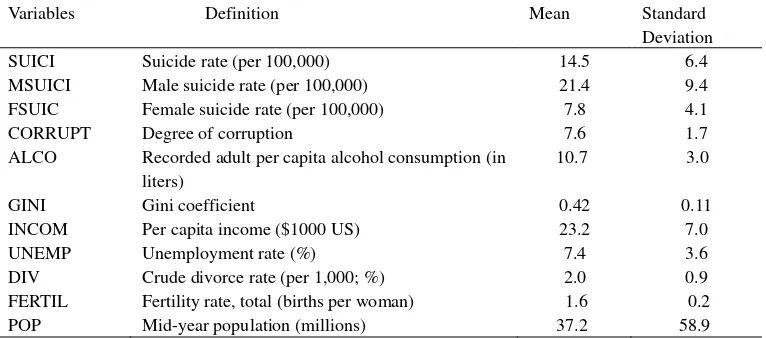
country size13. Table 1 provides definitions and descriptive statistics of the variables.
III. ESTIMATION RESULTS.
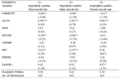
Results for the fixed effects models are given in Table 2, each corresponding to another
dependent variable (total, male, and female suicide rates). Regressions using the male suicide rates
as dependent variable are very similar to those on total suicide rates because males account for the
bulk of suicides. As indicated at the bottom of Table 2, the R squared values are higher in the models
13 Using adjusted suicide rates to control for differences in the structure of population is
6
in which the dependent variable is the total and male suicide rates. One might also conclude that
male suicide behaviour could be more responsive to socioeconomic conditions as opposed to female
behaviour. For the sake of brevity, we have focus on concentrated our focus on results for
CORRUPT and results where coefficients were statistically significant. As Table 2 shows the degree
of corruption is consistently negatively associated with suicide rates (in all regression models)..
Furthermore, its coefficient magnitudes are higher for total and male suicide rates than for female
suicide rates. In particular, the absolute value of CORRUPT coefficient was 0.65, suggesting that a
1 point increase in CORRUPT resulted in a 0.62 point decrease in suicide rates. The absolute value
of CORRUPT was 0.99 for male suicide rate, whereas the value was only 0.33 for female suicide
rate. This implies that a 1 point increase in CORRUPT resulted in a 0.99 point decrease in male
suicide rate, while a 1 point increase in CORRUPT resulted in a 0.33 point decrease in female
suicide rate. Hence, the effect of CORRUPT on male suicide rate was approximately three times
larger than that for female suicide rate. Regarding other control variables, our results are similar to
many other previous empirical studies using panel data. We found significant effects of divorce rate
on male suicides, and it has little effect on female suicide. Alcohol consumption is positively
associated with suicide rates, regardless of gender. Unemployment, income inequality and fertility
rates are found to be statistically insignificant in all regression models (for instance, Minoiu and
Andrés, 2008).
IV. CONCLUSION
Although suicide research is a multidisciplinary subject and socioeconomic factors are well
documented risk factors for suicide. Past research has neglected the role of quality governance
indicators. In particular, this study explored how corruption influences suicide rate using a panel
7
suicide rates are lower in countries with lower levels of corruption. Furthermore, its coefficient
magnitude is higher for male suicide rates than for female suicide rates. This implies that corruption
8
REFERENCES
Anbarci, N., Escaleras, M., & Register, C.A. (2006.) Traffic fatalities and public sector corruption.
Kyklos, 59(3), 327-344.
Anbarci,N., Escaleras,M. & Register,C.A. (2009). The ill effects of public sector corruption in the
water and sanitation sector, Land Economics, 85(2), 363-377.
Andrés, A.R., (2005). Income inequality, unemployment, and suicide: a panel data analysis of 15
European countries. Applied Economics, 3, 439-451.
Andvig, J.C. (2005). A House of Straw, Sticks or Bricks. Some Notes on Corruption Empirics, Paper
presented at the IV Global Forum on Fighting Corruption and Safeguarding Integrity, June
2005.
Babones, S.J., & Alvarez-Rivadulla, M.J. (2007). Standardized income inequality data for use in
cross-national research. Sociological Inquiry,77, 3-22.
Baltagi, B. (2005). Econometric Analysis of Panel Data, John Wiley and Sons.
Bertrand M, & Mullainathan S., (2001). Do people mean what they say? implications for
subjective survey data. American Economic Review, 91(2), 67–72.
Brainerd, E. (2001). Economic reform and mortality in the former Soviet Union: A study of the
suicide epidemic in the 1990s. European Economic Review, 45, 1007-1019.
Chen, J., Yun Jeong Choi, and Yasuyuki Sawada (2009). ‘How Is Suicide Different in Japan?’ Japan
and the World Econom,y21(2), 140-50.
Chuagn, H.L, & Huang, W.C. (2007). A Re-examination of the suicide rates in Taiwan. Social
Indicators Research, 83(3), 465-485.
Delavallade, C. (2006). Corruption and distribution of public spending in developing countries.
Journal of Economic Finance, 30, 222-239.
9
of European Economic Association,7, 539-549.
Escaleras,M., Anbarci,N., & Register,C.A. (2007). Public sector corruption and major earthquakes: A
potentially deadly interaction. Public Choice,132(1), 209-230.
Fischer, J.A.V., & Rodríguez, A. (2008). Political institutions and suicide: A regional analysis of
Switzerland. TWI Research Paper. Universitat Konstanz.
Helliwell, J.F., & Huang, H. (2008). How’s your government? International evidence linking good
government and well-being. British Journal of Political Science,38, 595-619.
Helliwell, J.F. (2007). Well-being and social capital. Does suicide post a puzzle? Social Indicators
Research, 455-496.
Kahn, M.E. (2005). The death toll from natural disasters: the role of income, geography, and
institutions. Review of Economics and Statistics, 87, 271-284.
Koivumaa-Honkanen H, Honkanen R, Viinamki H, Heikkil J, Kaprio J, & Koskenvuo M . (2001).
Life satisfaction and suicide: a 20-year follow-up study. The American Journal of Psychiatry,
158, 433-459.
Kunce, M., Anderson, A.L. (2002). The impact of socio-economic factors on state suicide rates: A
methodological note. Urban Studies,39, 155-162.
Lambsdorff, J.G., (2006). Causes and Consequences of Corruption: What do we know from a
Cross-Section of Countries? in S. Rose-Ackerman (ed.), International Handbook on the
Economics of Corruption, Cheltenham, UK: Edward Elgar, 2006, 3-51.
Mauro, P. (1995). Corruption and growth. The Quarterly Journal of Economics, 110(3), 681-712.
Minoiu, C., & Andres, A.R. (2008). The effect of public spending on suicide: Evidence from US
state data. Journal of Socio-Economics, 37(1), 237-261.
Noh, Y.H., (2009). Does unemployment increase suicide rates? The OECD panel evidence. Journal
10
Ott, J.C. (2010). Good governance and happiness in nations: Technical quality precedes democracy
and quality beats size. Journal of Happiness Studies, 11,353-368.
World Bank. (2006). World Development Indicators, CD-ROM, Washington, DC: World Bank.
Yamamura, E. (2010). The different impacts of socio-economic factors on suicide between males
8
Table 1
Variable definitions, means, and standard deviations (Observations = 102).
Variables Definition Mean Standard
Deviation
SUICI Suicide rate (per 100,000) 14.5 6.4
MSUICI Male suicide rate (per 100,000) 21.4 9.4
FSUIC Female suicide rate (per 100,000) 7.8 4.1
CORRUPT Degree of corruption 7.6 1.7
ALCO Recorded adult per capita alcohol consumption (in liters)
10.7 3.0
GINI Gini coefficient 0.42 0.11
INCOM Per capita income ($1000 US) 23.2 7.0
UNEMP Unemployment rate (%) 7.4 3.6
DIV Crude divorce rate (per 1,000; %) 2.0 0.9
FERTIL Fertility rate, total (births per woman) 1.6 0.2
9
Table 2
Panel data regression models. Fixed effects approach.
Explanatory variables
(1) Dependent variable: Total suicide rate
(2) Dependent variable: Male suicide rate
(3) Dependent variable: Female suicide rate
CORRUPT -0.65**
(-2.00)
-0.99* (-1.95)
-0.33* (-1.70)
ALCO 2.05***
(4.65)
3.26*** (4.79)
0.89*** (3.38)
GINI 5.83
(0.83)
13.6 (1.27)
-1.69 (-0.41)
INCOM -0.49**
(-2.23)
-0.86** (-2.55)
-0.14 (-1.06)
UNEMP 0.21
(1.21)
0.25 (0.97)
0.16 (1.59)
DIV 2.33**
(2.45)
4.33*** (2.95)
0.38 (0.67)
FERTIL -0.84
(-0.24)
-2.97 (-0.55)
1.22 (0.59)
Ln(POP) 0.41
(1.58)
0.57 (1.41)
0.27* (1.74)
R-squared (Within) 0.39 0.41 0.32
No. of observations 102 102 102
10
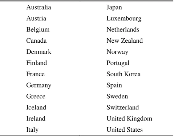
[image:14.595.136.419.135.355.2]APPENDIX.
Table A1. OECD countries in the regression analysis
Australia Japan
Austria Luxembourg
Belgium Netherlands
Canada New Zealand
Denmark Norway
Finland Portugal
France South Korea
Germany Spain
Greece Sweden
Iceland Switzerland
Ireland United Kingdom