http://www.scirp.org/journal/jwarp
ISSN Online: 1945-3108 ISSN Print: 1945-3094
Parameter Uncertainty Estimation by
Using the Concept of Ideal Data in GLUE
Approach
Junjun Zhu, Hong Du
College of Resources and Environment, South-Central University for Nationalities, Wuhan, China
Abstract
The hydrological uncertainty about NASH model parameters is investigated and addressed in the paper through “ideal data” concept by using the Genera-lized Likelihood Uncertainty Estimation (GLUE) methodology in an applica-tion to the small Yanduhe research catchment in Yangtze River, China. And a suitable likelihood measure is assured here to reduce the uncertainty coming from the parameters relationship. “Ideal data” is assumed to be no error for the input-output data and model structure. The relationship between para-meters k and n of NASH model is clearly quantitatively demonstrated based on the real data and it shows the existence of uncertainty factors different from the parameter one. Ideal data research results show that the accuracy of data and model structure are the two important preconditions for parameter estimation. And with suitable likelihood measure, the parameter uncertainty could be decreased or even disappeared. Moreover it is shown how distribu-tions of predicted discharge errors are non-Gaussian and vary in shape with time and discharge under the single existence of parameter uncertainty or under the existence of all uncertainties.
Keywords
Ideal Data, GLUE Methodology, Likelihood Measure, NASH Model, Yanduhe Catchment, Uncertainty Principles
1. Introduction
It is well known that the hydrological processes are very complicated and influ-enced by climate, weather, geographic and geomorphic conditions, underlying surface conditions and that it is very difficult to obtain the hydrographic features (precipitation, evaporation, discharge etc.) as well as the spatial and temporal
How to cite this paper: Zhu, J.J. and Du, H. (2017) Parameter Uncertainty Estima-tion by Using the Concept of Ideal Data in GLUE Approach. Journal of Water Re-source and Protection, 9, 65-82.
http://dx.doi.org/10.4236/jwarp.2017.91006
Received: June 8, 2016 Accepted: January 16, 2017 Published: January 19, 2017
Copyright © 2017 by authors and Scientific Research Publishing Inc. This work is licensed under the Creative Commons Attribution International License (CC BY 4.0).
distributions of hydrologic cycle features precisely. For all of these reasons, the accuracy of hydrological modeling will be influenced by these uncertainties.
The randomness and fuzziness of the hydrological phenomenon are the pri-mary causes for the modeling uncertainty. Hydrologists [1] [2] [3] [4] [5] have discussed such uncertainties originated by such causes as input-output data, hy-drological model structure and model parameter. In particular, the uncertainty of the hydrological data can be summarized as below: 1) Representativeness of the distribution character and mathematical expectation of hydrological features. Taking the rainfall as an example, as heterogeneityand variability of the precipi-tation spatial distribution, maybe the information obtained in fixed rainfall sta-tion network is inaccurate to be used as mean value in an area; 2) measurement error. As the existence of the instrument error or fault and observer’s operation or evaluation error for the flood monitoring system, there must be input-output error for modeling; 3) lack reliable information for some hydrologic features.
Analogously, the model uncertainty can be summarized as below: 1) Since the knowledge limitations of hydrological processes, the descriptions of such pro- cesses may be approximate or unreasonable; 2) most mathematical and physical functions used in complex processes calculation are simplified; 3) many models cannot reflect the influence of environmental factors, such as global climate and land cover change due to human activities, to the run off process; 4) effective computing methods are needed. The rainfall-runoff is a continuous process that is simulated by the model in a discrete way causing inevitable errors. Besides, different discrete ways could have different influences; 5) model parameter val-ues are difficult to be obtained by either measurement or prior estimation.
The research of parameter uncertainty is fundamental and meaningful. Once the hydrological model is confirmed, the parameters will be the key point for the modeling validity: the modeling will stand or fall according to the parameters. Premier researches about modeling uncertainty are mainly about model para-meters but with the existence of other uncertainties, such as the Generalized Li-kelihood Uncertainty Estimation (GLUE) methodology [4] [6], the Shuffled Complex Evolution Metropolis algorithm (SCEM-UA) [7], and the Markov Chain Monte Carlo (MCMC) method [8]. All these methods were aimed to represent the parameter uncertainty but ignored the influence of other uncer-tainty factors. Therefore, the key point now is how to avoid or decrease the in-fluences of input-output data uncertainty and model structure uncertainty for the exact estimation of the parameters. For this, “ideal data” is proposed in the paper to do the parameter uncertainty and interaction estimation by using GLUE methodology. And meanwhile the likelihood measure is also studied here. The proposed approach is applied to the well-known NASH runoff model con-sidering as case study in Yanduhe basin of Yangtze River, China.
2. Theoretical Background
2.1. The GLUE Methodology
The GLUE procedure recognizes the equivalence of different sets of parameters in the calibration of models. It is based upon running a model with different sets of parameter values chosen randomly from the specified spatial distributions. Many papers have applied this methodology and emphasize the effects of the li-kelihood measure in the whole applying process [9] [10]. The term “likelihood” was used in a general sense, as a fuzzy, belief, or possible measure of how well the model conforms to the observed behavior of the system [4], yet not in the re-stricted sense of maximum likelihood theory which is developed under specific assumptions of zero mean, normally distributed errors [11] [12]. Moreover, it is subjective to choose a suitable threshold for the likelihood measure to identify the behavior of the model. In the past studies, usually the threshold was chosen subjectively on the scale of some summary goodness of fit index [13] [14] [15]. And the GLUE method is used well in uncertainty research [16] [17].
Here in the application of GLUE methodology, for each set of parameters, whether the model is behavioral or not is determined by the likelihood value on a basis of comparing predicted and observed responses.
The requirements of the GLUE procedure are given as follows:
1) A formal definition of a likelihood measure. At this stage it is worth noting that a formal definition is required but the choice of a likelihood measure will be inherently subjective.
2) An appropriate definition of the initial range and the distributions of the parameters to be considered for a particular model.
3) Definition of a feasible threshold value.
2.2. NASH Model
The NASH model [18] [19] [20] [21] is a conceptual hydrological concentration model developed by Nash, J.E., and it is widely used in the watershed concentra-tion simulaconcentra-tion [22] [23]. In the model, the research basin is divided into a series of identical reservoirs, and the reallocation of the net rainfall in the catchment is assimilated to be an adjustment of the reservoirs. So the instantaneous unit hy-drograph (IUH) can be deduced as Eq. (1):
( )
1 1 1
( )
n k k
u t e
k n t
− −
=
Γ (1)
where u t
( )
is the y-coordinate of instantaneous unit hydrograph; Γ( )
n is the Gamma function; n reflects the regulation and storage capacity of the basin, and it could be the number of the reservoirs, termed shape parameter; k is the storage-discharge parameter of the reservoirs, termed scale parameter. The Nash model with its clear conception and simple structure has been used extensively in flood forecasting [24] [25].1 ( )
0 1
( ) ( )
( 1)!
n t
t
k t
Q t e h d
n k k
τ
τ − − − τ τ
−
=
−
∫
(2)2.3. Generation of the Ideal Data
To avoid the input-output uncertainty and the model structure uncertainty, the concept of “ideal data” is proposed to do the research of model parameters un-certainty.
On the basis of the physical interpretation of the hydrological model and the characteristics of the research catchment, the model parameter spaces can be determined based on the prior information. Choose one set of parameters ran-domly in the parameter spaces as the “true parameter values”. First assume the input data has no error, then the input is called “ideal input”, and the “ideal output” can be calculated by using the “true parameter values” in the model.
For NASH model, the input is net rainfall and output is flow at the basin out-let.
3. Case Study and Results
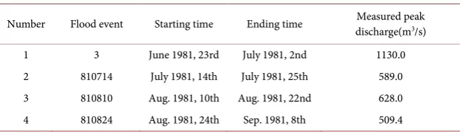
The Yanduhe catchment in upper reaches of the Yangtze River basin covers a drainage area of 601 km2 where the annual average rainfall is about 1337 mm, and the runoff mainly comes from the rainfall. In this research catchment, four flood events are used in the case study (Table 1).
For NASH model, based on the physical interpretation and the catchment da-ta, the spaces of the two parameters are k [0.5 - 4] and n [0.5 - 5]. The input is the net rainfall and the output is the surface runoff. Here the net rainfall is cal-culated by XAJ rainfall-runoff model [26]. In real data research, the error com-ing from XAJ model is assumed as input error of NASH model. In the applica-tion of GLUE methodology, it is done by Monte Carlo simulaapplica-tion, using uniform sampling in the specified parameter range.
In rainfall-runoff modeling we are often evaluating the errors in simulating a time series of discharge or other observed data. A classical statistical measure for evaluating goodness of fit based on the sum of squared errors or error variance is suggested by Nash and Sutcliffe (1970) in the form
2
1 1 2
L ε
ο
σ σ
[image:4.595.208.539.637.732.2]= − (3)
Table 1. The four flood events.
Number Flood event Starting time Ending time discharge(mMeasured peak 3/s)
1 3 June 1981, 23rd July 1981, 2nd 1130.0
2 810714 July 1981, 14th July 1981, 25th 589.0
3 810810 Aug. 1981, 10th Aug. 1981, 22nd 628.0
where 2
ε
σ is the variance of the errors; 2
ο
σ is the variance of the observations. Another measure based on the sum of squared errors is the inverse error measure suggested by Box and Tiao (1992) in the form:
( )
22( )
N
L N σε
−
= (4)
where N is a shaping parameter.
Here two likelihood measures were chosen for model and parameter uncer-tainty research by GLUE methodology.
3.1. GLUE Research under Real Data
The GLUE methodology has been first applied to the real data (observed dis-charge) research with likelihood measure L1. In this study the choice of a model efficiency rejection criterion (<0) has been included, which assure all of the possible modeling results can be contained.
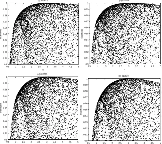
Scatter plots of parameters k and n based on the likelihood measure L1are reported in Figure 1 and Figure 2 which show the effects of using different flood events with real input-output data. It can be seen that good and poor simulations are available virtually throughout the parameter ranges, and the effects of dif-ferent flood events for parameters k and n are seen clearly. It can be inferred that there is uncertainty of input-output data or others simultaneously to influ-ence the distributions of the scatter plots.
The results shown in Figure 1 and Figure 2 suggest that the parameter re-sponse surfaces are very complex and for different data that is for different events they vary showing the uncertainty of data.
It is difficult in rainfall-runoff modeling to bracket all the discharge observa-tions (or other predicted variables) within 90% of the calculated confidence bounds, as seen in Figure 3, the discharge is often outside of the 90% confidence bounds, which furthermore proves the data limitations as well as the model structure limitations.
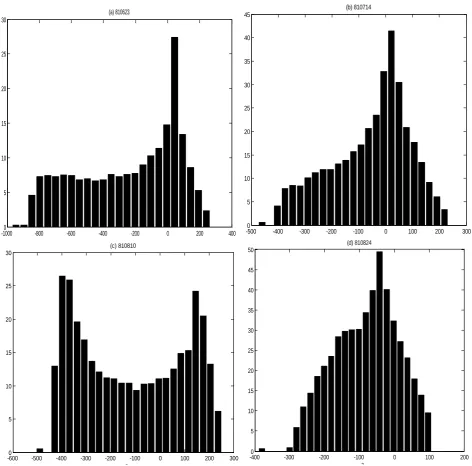
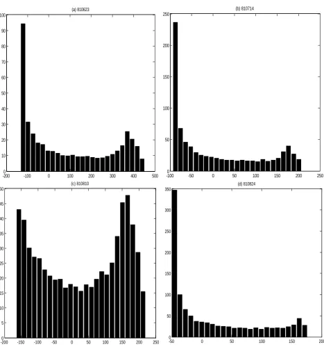
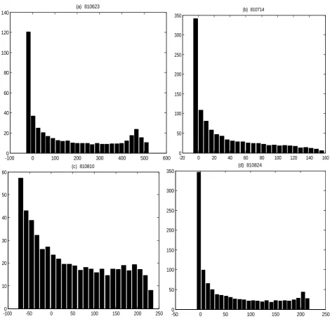
Figures 4-6 show the distribution of errors Etp, Etp+10, Etp−10, computed
considering the four flood events under real data research, referring to peak dis-charge, Qtp, discharge 10 hours after peak time, Qtp+10, discharge 10 hours
be-fore peak time, Qtp−10, respectively. It is easy to see from the figures that the dis-
tributions are non-Gaussian and vary in shape through time under the existence of parameter uncertainty, data uncertainty and model structure uncertainty.
3.2. GLUE Research under Ideal Data
Then the GLUE methodology has been applied in parameter uncertainty re-search by proposing the “ideal data” to avoid the influence of other uncertainty factors. Following the above generation steps of the “ideal data”, one set of pa-rameters is chosen as the “true parameter values”:
(
n=3.115,k=1.203)
, thenFigure 1. Scatter plots of efficiency results for parameter k in the four real flood events.
Figure 2. Scatter plots of efficiency results for parameter n in the four real flood events.
0.5 1 1.5 2 2.5 3 3.5 4
0.2 0.3 0.4 0.5 0.6 0.7 0.8 0.9 1 k (h) lik e lih o o d (a) 810623
0.5 1 1.5 2 2.5 3 3.5 4
0.4 0.5 0.6 0.7 0.8 0.9 1 k(h) lik e lih o o d (b) 810714
0.5 1 1.5 2 2.5 3 3.5 4
0.1 0.2 0.3 0.4 0.5 0.6 0.7 0.8 0.9 k (h) lik e lih o o d (c) 810810
0 1 2 3 4
0 0.2 0.4 0.6 0.8 1 k(h) lik e lih o o d (d) 810824
0 1 2 3 4 5
0.2 0.3 0.4 0.5 0.6 0.7 0.8 0.9 1 n lik e lih o o d (a) 810623
0 1 2 3 4 5
0.4 0.5 0.6 0.7 0.8 0.9 1 n lik e lih o o d (b) 810714
0 1 2 3 4 5
0.1 0.2 0.3 0.4 0.5 0.6 0.7 0.8 0.9 1 n lik e lih o o d (c) 810810
0 1 2 3 4 5
[image:6.595.212.537.407.706.2]Figure 3. Ninety percent uncertainty bounds for simulations of the four real flood events in the Yanduhe catchment.
0 20 40 60 80 100 120 140 160 180
0 1356
t(h)
Q
(m
3/s)
0 20 40 60 80 100 120 140 160 180
0
10
20
30
40
50
60
70
80 t(h)
mm
(a) 810623
real discharge lower bounds upper bounds
rain
0 50 100 150 200 250
0 706.8
t(h)
Q
(m
3 /s)
0 50 100 150 200 250
0
10
20
30
40
50
60
70
80
t(h)
mm
(b) 810714
real discharge lower bounds upper bounds
rain
0 50 100 150 200 250
0 753.6
t(h)
Q
(m
3/s)
0 50 100 150 200 250
0
10
20 30
40 50
60
70
80 t(h)
mm
(c) 810810
real discharge lower bounds upper bounds
rain
0 50 100 150 200 250 300 350
0 611.28
t(h)
Q
(m
3 /s)
(d) 810824
0 50 100 150 200 250 300 350
0
10
20
30
40
50
60 70
80 t(h)
mm
real discharge lower bounds upper bounds
Figure 4. Error distributions at the point of tp in the four real flood events.
model structure, under which situation the NASH parameter uncertainty is si-mulated by GLUE methodology. Here the choice of a high model efficiency re-jection criterion (<0.90) has been included, since this is one way of trying to es-timate the relationship of the two parameters.
Figure 7 and Figure 8 are scatter plots of efficiency results for parameters k and n under ideal data. It is easy to see that each parameter has very similar efficiency under different flood events. By Comparing Figure 7 and Figure 8
with Figure 1 and Figure 2, it also can be inferred that there are no other un-certainty factors affecting the parameters unun-certainty research.
Comparing Figure 9 to Figure 3, it is easy to prove that all of the ideal dis-charges in NASH modeling are bracketed within the 90% calculated uncertainty
-10000 -800 -600 -400 -200 0 200 400
5 10 15 20 25 30
(a) 810623
-5000 -400 -300 -200 -100 0 100 200 300
5 10 15 20 25 30 35 40 45
(b) 810714
-6000 -500 -400 -300 -200 -100 0 100 200 300
5 10 15 20 25 30
(c) 810810
3
-4000 -300 -200 -100 0 100 200
5 10 15 20 25 30 35 40 45 50
(d) 810824
Figure 5. Error distributions at the point of tp+10 in the four real flood events.
bounds, as shown in Figure 9. And for different flood events with ideal input data, the results are consistent, which demonstrate that there are no other un-certainty factors except the model parameters and assure the research accuracy of the model parameter uncertainty and correlation estimation. Obviously, the ideal data can assure the accuracy of the parameter uncertainty research.
Figure 10 shows the response surface of parameters k and n with good-ness of fit represented as contours and suggests the obvious correlation and un-certainty of the two parameters.
Figure 11 gives the scatter plots of parameters k and n with likelihood
-2000 -100 0 100 200 300 400 500
10 20 30 40 50 60 70 80 90 100
(a) 810623
-1000 -50 0 50 100 150 200 250
50 100 150 200 250
(b) 810714
-2000 -150 -100 -50 0 50 100 150 200 250
5 10 15 20 25 30 35 40 45 50
(c) 810810
-50 0 50 100 150 200
0 50 100 150 200 250 300 350
Figure 6. Error distributions at the point of tp−10 in the four real flood events.
value greater than 0.98 trying to find the ridge line, from which we can assume that the distributions of the scatter plots can be matched by the function as be-low:
n k⋅ =C (5)
where C is equal to 3.82.
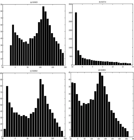
For the ideal data analysis, the uncertainty assessment refers only to the pa-rameters, so it is accurate to analyze the error distributions of the discharges as the parameter errors. Same as the real data research, Figures 12-14 show for
-50 0 50 100 150 200
0 10 20 30 40 50 60 70 80 90
(a) 810623
-10 -5 0 5 10 15 20
0 500 1000 1500 2000 2500 3000 3500
(b) 810714
-50 0 50 100 150 200
0 10 20 30 40 50 60 70 80 90 100
(c) 810810
-50 0 50 100 150 200 250 300 350 400
0 5 10 15 20 25 30 35 40 45
Figure 7. Scatter plots of efficiency results for parameter k in the four ideal flood events.
Figure 8. Scatter plots of efficiency results for parameter n in the four ideal flood events.
0.5 1 1.5 2 2.5 3 3.5 4
0.9 0.91 0.92 0.93 0.94 0.95 0.96 0.97 0.98 0.99 1 k (h) li k el ihood (a) 810623
0.5 1 1.5 2 2.5 3 3.5 4
0.9 0.91 0.92 0.93 0.94 0.95 0.96 0.97 0.98 0.99 1 k (h) li k el ihood (b) 810714
0.5 1 1.5 2 2.5 3 3.5 4
0.9 0.91 0.92 0.93 0.94 0.95 0.96 0.97 0.98 0.99 1 k (h) li k el ihood (c) 810810
0.5 1 1.5 2 2.5 3 3.5 4
0.9 0.91 0.92 0.93 0.94 0.95 0.96 0.97 0.98 0.99 1 k (h) li k el ihood (d) 810824
0.5 1 1.5 2 2.5 3 3.5 4 4.5 5 0.9 0.91 0.92 0.93 0.94 0.95 0.96 0.97 0.98 0.99 1 n li k el ihood (a) 810623
0.5 1 1.5 2 2.5 3 3.5 4 4.5 5 0.9 0.91 0.92 0.93 0.94 0.95 0.96 0.97 0.98 0.99 1 n li k el ihood (b) 810714
0.5 1 1.5 2 2.5 3 3.5 4 4.5 5
0.9 0.91 0.92 0.93 0.94 0.95 0.96 0.97 0.98 0.99 1 n li k el ihood (c) 810810
0.5 1 1.5 2 2.5 3 3.5 4 4.5 5
[image:11.595.211.537.409.698.2]Figure 9. Ninety percent uncertainty bounds for simulations of the four ideal flood events in the Yanduhe catchment.
Figure 10. Ideal data analysis: Response surface for parameter k and n with goodness of fit represented as contours.
each flood event the error distributions of three discharge values, which demon-strate how distributions are non-Gaussian and vary in shape through time under the single existence of parameters uncertainty.
Figure 15 is the research result under idea data based on the likelihood L2 with parameter N = 20. For the four flood events, all of the “real parameters of model” are obtained in the figure.
0 20 40 60 80 100 120 140 160 180
0 200 400 600 800 1000 1200 1400 t(h) Q (m 3/s )
(a) 810623
0 20 40 60 80 100 120 140 160 180
0 10 20 30 40 50 60 70 t(h) ideal discharge lower bounds upper bounds rain
0 50 100 150 200 250
0 100 200 300 400 500 600 700 t(h) Q (m 3/s )
(b) 810714
0 50 100 150 200 250
0 10 20 30 40 50 60 70 t(h) ideal discharge lower bounds upper bounds rain
0 50 100 150 200 250
0 100 200 300 400 500 600 700 800 t(h) (c) 810810
0 50 100 150 200 250
0 10 20 30 40 50 60 70 80 t(h) mm ideal discharge lower bounds upper bounds rain
0 50 100 150 200 250 300 350
0 100 200 300 400 500 600 t(h) Q (m 3/s )
(d) 810824
0 50 100 150 200 250 300 350
0 10 20 30 40 50 60 t(h) ideal discharge lower bounds upper bounds rain
0.5 1 1.5 2 2.5 3 3.5 4
0.5 1 1.5 2 2.5 3 3.5 4 4.5 5 k n 810623
Figure 11. Response surface for k and n in the four ideal flood events.
Figure 12. Error distributions at the point of tp in the four ideal flood events.
0.5 1 1.5 2 2.5 3
1 1.5 2 2.5 3 3.5 4 4.5 5
k
n
810623 810714 820810 820824
-10000 -800 -600 -400 -200 0 200
5 10 15 20 25
3
f(E
tp
)
(a) 810623
-2000 -150 -100 -50 0 50
10 20 30 40 50 60
f(E
tp
)
(b) 810714
-4000 -300 -200 -100 0 100 200
5 10 15 20 25 30
f(E
tp
)
(c) 810810
-4500 -400 -350 -300 -250 -200 -150 -100 -50 0 50
5 10 15 20 25 30 35 40 45 50
f(E
tp
)
[image:13.595.69.518.320.713.2]Figure 13. Error distributions at the point of tp+10 in the four ideal flood events.
4. Conclusions
The paper proposes the concept of “ideal data” for parameter uncertainty as-sessment. The analysis is carried out for the NASH model parameters
k
andn
in Yanduhe catchment of Yangtze River, China, by GLUE methodology with both of “real” and “ideal” data.In idea data research, the consistent results from the different flood events demonstrate that there are no other uncertainty factors except the model pa-ra-meters, which assure the research accuracy of the model parameters uncer-tainty and correlation estimation. Obviously with the ideal data, the estimation for parameters uncertainty is accurate and reliable. And with suitable likelihood measure, the parameter uncertainty could be disappeared. The results also clear-ly show that under ideal data, the real parameter set is obtained, but the results
-1000 0 100 200 300 400 500 600
20 40 60 80 100 120 140
(a) 810623
-20 0 20 40 60 80 100 120 140 160
0 50 100 150 200 250 300 350
p
(b) 810714
-1000 -50 0 50 100 150 200 250
10 20 30 40 50 60
p
(c) 810810
-50 0 50 100 150 200 250
0 50 100 150 200 250 300 350
also show that the distributions of errors are not Gaussian distribution as which are always assumed.
[image:15.595.61.537.220.708.2]In real data research, when the model is confirmed the uncertainty due to both parameter uncertainty and data uncertainty. And the ideal data research show that the parameter uncertainty depends on the relationship between the two parameters. So the way to deal with the parameter uncertainty is how to re-duce the correlation of the two parameters or confirm their correlation by con-stant function. But with likelihood L2 the uncertainty from the parameters cor-relation could be decreased in real data research
Figure 14. Error distributions at the point of tp−10 in the four ideal flood events.
-2000 -150 -100 -50 0 50
20 40 60 80 100 120
(a) 810623
-20 0 20 40 60 80 100 120
0 50 100 150 200 250 300
(b) 810714
-1200 -100 -80 -60 -40 -20 0 20 40
20 40 60 80 100 120
(c) 810810
-3500 -300 -250 -200 -150 -100 -50 0 50 100
5 10 15 20 25 30 35 40 45
3
Figure 15. Response surface for parameters k and n under ideal data with likelihood L2.
0.5 1 1.5 2 2.5 3 3.5 4
0.5 1 1.5 2 2.5 3 3.5 4 4.5 5
X: 1.2 Y: 3.11
k(h)
n
(a) 810623
0.5 1 1.5 2 2.5 3 3.5 4
0.5 1 1.5 2 2.5 3 3.5 4 4.5 5
X: 1.2 Y: 3.11
k(h)
n
(b) 810714
0.5 1 1.5 2 2.5 3 3.5 4
0.5 1 1.5 2 2.5 3 3.5 4 4.5 5
X: 1.2 Y: 3.11
k(h)
n
(c) 810810
0.5 1 1.5 2 2.5 3 3.5 4
0.5 1 1.5 2 2.5 3 3.5 4 4.5 5
X: 1.2 Y: 3.11
k(h)
n
The distributions of errors from model structure uncertainty, data uncertainty and model parameter uncertainty or from single model parameter uncertainty are non-Gaussian, and furthermore, changeable in each rainfall-runoff event. Meanwhile for different flood events they are also different. So it is not reasona-ble to assume the errors with this certain kind of distribution. Comparing these to the results from ideal data estimation, the mixed uncertainties make the error distributions more complicated.
Suitable likelihood measure is very important for uncertainty estimation and parameters determination. While the accurate data and perfect model structure are the two important factors for C. They are the preconditions for the estima-tion of model parameter uncertainty and interacestima-tion.
Acknowledgements
This study was financially supported by the Provincial Natural Science Founda-tion of Hubei (BZY14026) and the Fundamental Research Funds for the Central Universities, South-Central University for Nationalities (CZQ13006).
References
[1] Kuczera, G. (1983) Improved Parameter Inference in Catchment Models:
Evaluat-ing Parameter Uncertainty. Water Resources Research, 19, 1151-1162.
https://doi.org/10.1029/WR019i005p01151
[2] Melching, C.S. (1995) Reliability estimation. In: Singh, V.P., Ed., Computer Models
of Watershed Hydrology. Water Resources Publications, Highlands Ranch, CO, Chapter 3.
[3] Zhao, R.J. (1989) Comparative Analysis Research of Hydrology Models. Journal of
China Hydrology, No. 6, 1-5.
[4] Beven, K.J. and Binley, A. (1992) The Future of Distributed Models: Model
Calibra-tion and Uncertainty PredicCalibra-tion. Hydrology Processes, 6, 279-298.
https://doi.org/10.1002/hyp.3360060305
[5] Rui, X.F., Liu F.G. and Xin, Z.X. (2007) Advances in Hydrology and Some Frontier
Problems. Advances in Science and Technology of Water Resources, 27, 75-79.
[6] Page, T., Whyatt, J.D., Beven, K.J. and Metcalfe, S.E. (2004) Uncertainty in
Mod-elled Estimates of Acid Deposition across Wales: A GLUE Approach. Atmospheric
Environment, 38, 2079-2090. https://doi.org/10.1016/j.atmosenv.2004.01.029
[7] Vrugt, J.A., Gupta, H.V., Bouten, W. and Sorooshian, S. (2003) A Shuffled Complex
Evolution Metropolis Algorithm for Optimization and Uncertainty Assessment of
Hydrologic Model Parameters. Water Resources Research, 39, 1201.
https://doi.org/10.1029/2002WR001642
[8] Kuczera, G. and Parent, E. (1998) Monte Carlo Assessment of Parameter
Uncer-tainty in Conceptual Catchment Models: The Metropolis Algorithm. Journal of
Hydrology, 211, 69-85. https://doi.org/10.1016/S0022-1694(98)00198-X
[9] Beven, K.J. and Freer, J. (2001) Equifinality, Data Assilimilation, and Uncertainty
Estimation in Mechanistic Modeling of Complex Environmental Systems Using the
GLUE Methodology. Journal of Hydrology, 249, 11-29.
https://doi.org/10.1016/S0022-1694(01)00421-8
[10] Blasone, R.S., Vrugt, J.A., Madsen, H., Rosbjerg, D., Robinson, B.A., Zyvoloski, G.A.
Markov Chain Monte Carlo Sampling. Advances in Water Resources, 31, 630-648.
https://doi.org/10.1016/j.advwatres.2007.12.003
[11] Sorooshian, S. (1981) Parameter Estimation of Rainfall-Runoff Models with
Hete-roscedastic Stream Errors: The Noninformative Data Case. Journal of Hydrology,
52, 127-138. https://doi.org/10.1016/0022-1694(81)90099-8
[12] Sorooshian, S. and Dracup, J.A. (1980) Stochastic Parameter Estimation Procedure
for Hydrologic Rainfall-Runoff Models: Correlated and Heteroscedastic Error Cas-es. Water Resources Research, 16, 430-442.
https://doi.org/10.1029/WR016i002p00430
[13] Freer, J., Beven, A.M. and Ambroise, B. (1996) Bayesian Estimation of Uncertainty
in Runoff Prediction and the Value of Data: An Application of the GLUE Approach.
Water Resources Research, 32, 2161-2173. https://doi.org/10.1029/95WR03723
[14] Candela, A., Noto, L.V. and Aronica, G. (2005) Influence of Surface Roughness in
Hydrological Response of Semiarid Catchments. Journal of Hydrology, 313, 119-
131. https://doi.org/10.1016/j.jhydrol.2005.01.023
[15] Choi, H.T. and Beven, K.J. (2007) Multi-Period and Multi-Criteria Model
Condi-tioning to Reduce Prediction Uncertainty in an Application of TOPMODEL within
the GLUE Framework. Journal of Hydrology, 332, 316-336.
https://doi.org/10.1016/j.jhydrol.2006.07.012
[16] Wu, H.J. and Chen, B. (2015) Evaluating Uncertainty Estimates in Distributed
Hy-drological Modeling for the Wenjing River Watershed in China by GLUE, SUFI-2,
and ParaSol Methods. Ecological Engineering, 76, 110-121.
https://doi.org/10.1016/j.ecoleng.2014.05.014
[17] Xue, C., Chen, B. and Wu, H.J. (2013) Parameter Uncertainty Analysis of Surface
Flow and Sediment Yield in the Huolin Basin in China. Journal of Hydrological
En-gineering, 19, 1224-1236. https://doi.org/10.1061/(ASCE)HE.1943-5584.0000909
[18] Nash, J.E. (1957) The Form of the Instantaneous Unit Hydrograph.
Publica-tions—International Association of Hydrological Sciences, 45, 114-121.
[19] Nash, J.E. (1958) Determining Runoff from Rainfall. Proceedings of the Institution
of Civil Engineers, 10, 163-184.
[20] Nash, J.E. (1959) Systematic Determination of Unit Hydrograph Parameters.
Jour-nal of Geophysical Research, 64, 111-115. https://doi.org/10.1029/JZ064i001p00111
[21] Nash J.E. (1960) A Unit Hydrograph Study, with Particular Reference to British
Catchments. Proceedings of the Institution of Civil Engineers, 17, 249-282.
https://doi.org/10.1680/iicep.1960.11649
[22] Lee, Y.H. and Singh, V.P. (1998) Application of the Kalman Filter to the Nash
Model. Hydrological Processes, 12, 755-767.
[23] Kalinin, G.P. and Milyukov, P.I. (1958) On the Computation of Unsteady Flow in
Open Channels. Meteorological Gidrologia, 10, 10-18.
[24] Choi, Y., Lee, G. and Kim, J. (2011) Estimation of the Nash Model Parameters
Based on the Concept of Geomorphologic Dispersion. Journal of Hydrological
En-gineering, 16, 806-817. https://doi.org/10.1061/(ASCE)HE.1943-5584.0000371
[25] Li, C., Guo, S. and Zhang, W. (2008) Use of Nash’s IUH and DEMs to Identify the
Parameters of an Unequal-Reservoir Cascade IUH Model. Hydrological Processes,
22, 4073-4082. https://doi.org/10.1002/hyp.7009
[26] Zhao, R.J, Wang, P.L. and Hu, F.B. (1992) Relations between Parameter Values and
Corresponding Natural Conditions of Xinanjiang Model. Journal of Hohai
Submit or recommend next manuscript to SCIRP and we will provide best service for you:
Accepting pre-submission inquiries through Email, Facebook, LinkedIn, Twitter, etc. A wide selection of journals (inclusive of 9 subjects, more than 200 journals)
Providing 24-hour high-quality service User-friendly online submission system Fair and swift peer-review system
Efficient typesetting and proofreading procedure
Display of the result of downloads and visits, as well as the number of cited articles Maximum dissemination of your research work
Submit your manuscript at: http://papersubmission.scirp.org/