Approach to a Proof of the Riemann Hypothesis by the Second Mean Value Theorem of Calculus

http://www.scirp.org/journal/apm ISSN Online: 2160-0384 ISSN Print: 2160-0368

Approach to a Proof of the Riemann Hypothesis by

the Second Mean-Value Theorem of Calculus

Alfred Wünsche

Humboldt-Universität Berlin, Institut für Physik, Nichtklassische Strahlung (MPG), Berlin, Germany

Abstract

By the second mean-value theorem of calculus (Gauss-Bonnet theorem) we prove that the class of functions Ξ

( )

z with an integral representation of the form

( ) ( )

0 du u ch uz

+∞

Ω

∫

with a real-valued function Ω

( )

u ≥0 which is non-increasing and decreases in infinity more rapidly than any exponential functions exp

(

−λu

)

,

0

λ> _{possesses zeros only on the imaginary axis. The Riemann zeta function} ζ

( )

s

as it is known can be related to an entire function ξ

( )

s with the same non-trivial

zeros as ζ

( )

s . Then after a trivial argument displacement 1

2

s↔ = −z s we relate it

to a function Ξ

( )

z with a representation of the form

( )

( ) ( )

0 d ch z +∞ u u uz

Ξ =

_∫

Ω

where Ω

( )

u is rapidly decreasing in infinity and satisfies all requirements

necessary for the given proof of the position of its zeros on the imaginary axis z=iy

by the second mean-value theorem. Besides this theorem we apply the Cauchy- Riemann differential equation in an integrated operator form derived in the Appendix B. All this means that we prove a theorem for zeros of Ξ

( )

z on the

imaginary axis z=iy for a whole class of function Ω

( )

u which includes in this

way the proof of the Riemann hypothesis. This whole class includes, in particular, also the modified Bessel functions Iν

( )

z for which it is known that their zeros lie

on the imaginary axis and which affirms our conclusions that we intend to publish at another place. In the same way a class of almost-periodic functions to piece-wise constant non-increasing functions Ω

( )

u belong also to this case. At the end we

give shortly an equivalent way of a more formal description of the obtained results using the Mellin transform of functions with its variable substituted by an operator.

Keywords

Riemann Hypothesis, Riemann Zeta Function, Xi Function, Gauss-Bonnet

How to cite this paper: Wünsche, A. (2016) Approach to a Proof of the Riemann Hypothesis by the Second Mean-Value The- orem of Calculus. Advances in Pure Ma-thematics, 6, 972-1021.

http://dx.doi.org/10.4236/apm.2016.613074

Received: July 9, 2016 Accepted: December 17, 2016 Published: December 20, 2016

Copyright © 2016 by author and Scientific Research Publishing Inc. This work is licensed under the Creative Commons Attribution International License (CC BY 4.0).

http://creativecommons.org/licenses/by/4.0/

Theorem, Mellin Transformation

1. Introduction

The Riemann zeta function ζ

( )

s which basically was known already to Euler

establishes the most important link between number theory and analysis. The proof of the Riemann hypothesis is a longstanding problem since it was formulated by Riemann [1] in 1859. The Riemann hypothesis is the conjecture that all nontrivial zeros of the Riemann zeta function ζ

( )

s for complex s= +σ it are positioned on the line

1 i 2

s= + t that means on the line parallel to the imaginary axis through real value

1 2

σ= in the complex plane and in extension that all zeros are simple zeros [2]-[17] (with extensive lists of references in some of the cited sources, e.g., ([4] [5] [9] [12] [14]). The book of Edwards [5] is one of the best older sources concerning most problems connected with the Riemann zeta function. There are also mathematical tables and chapters in works about Special functions which contain information about the Riemann zeta function and about number analysis, e.g., Whittaker and Watson [2] (chap. 13), Bateman and Erdélyi [18] (chap. 1) about zeta functions and [19] (chap. 17) about number analysis, and Apostol [20][21] (chaps. 25 and 27). The book of Borwein, Choi, Rooney and Weirathmueller [12] gives on the first 90 pages a short account about achievements concerning the Riemann hypothesis and its consequences for number theory and on the following about 400 pages it reprints important original papers and expert witnesses in the field. Riemann has put aside the search for a proof of his hypothesis “after some fleeting vain attempts” and emphasizes that “it is not necessary for the immediate objections of his investigations” [1] (see [5]). The Riemann hypothesis was taken by Hilbert as the 8-th problem in his representation of 23 fundamental unsolved problems in pure mathematics and axiomatic physics in a lecture hold on 8 August in 1900 at the Second Congress of Mathematicians in Paris [22][23]. The vast experience with the Riemann zeta function in the past and the progress in numerical calculations of the zeros (see, e.g., [5][10][11][16][17][24][25]) which all confirmed the Riemann hypothesis suggest that it should be true corresponding to the opinion of most of the specialists in this field but not of all specialists (arguments for doubt are discussed in [26]).

The Riemann hypothesis is very important for prime number theory and a number of consequences is derived under the unproven assumption that it is true. As already said a main role plays a function ζ

( )

s which was known already to Euler for real

variables s in its product representation (Euler product) and in its series re-

presentation (now a Dirichlet series) and was continued to the whole complex s-plane

parallel to the imaginary axis and intersecting the real axis at 1 2

s= . For the true

hypothesis the representation of the Riemann zeta function after exclusion of its only singularity at s=1 and of the trivial zeros at s= −2 ,n n

(

=1, 2,

)

on the negative real axis is possible by a Weierstrass product with factors which only vanish on the critical line 1

2

σ = _{. The function which is best suited for this purpose is the so-called xi} function ξ

( )

s which is closely related to the zeta function ζ

( )

s and which was also

introduced by Riemann [1]. It contains all information about the nontrivial zeros and only the exact positions of the zeros on this line are not yet given then by a closed formula which, likely, is hardly to find explicitly but an approximation for its density was conjectured already by Riemann [1] and proved by von Mangoldt [27]. The “(pseudo)-random” character of this distribution of zeros on the critical line remembers somehow the “(pseudo)-random” character of the distribution of primes where one of the differences is that the distribution of primes within the natural numbers becomes less dense with increasing integers whereas the distributions of zeros of the zeta function on the critical line becomes more dense with higher absolute values with slow increase and approaches to a logarithmic function in infinity.

There are new ideas for analogies to and application of the Riemann zeta function in other regions of mathematics and physics. One direction is the theory of random matrices [16][24] which shows analogies in their eigenvalues to the distribution of the nontrivial zeros of the Riemann zeta function. Another interesting idea founded by Voronin [28] (see also [16][29]) is the universality of this function in the sense that each holomorphic function without zeros and poles in a certain circle with radius less

1

2 can be approximated with arbitrary required accurateness in a small domain of the zeta function to the right of the critical line within 1 1

2≤ ≤s . An interesting idea is elaborated in articles of Neuberger, Feiler, Maier and Schleich [30][31]. They consider a simple first-order ordinary differential equation with a real variable t (say the time)

for given arbitrary analytic functions f z

( )

where the time evolution of the function

for every point z finally transforms the function in one of the zeros f z

( )

=0 of this

function in the complex z-plane and illustrate this process graphically by flow curves

which they call Newton flow and which show in addition to the zeros the separatrices of the regions of attraction to the zeros. Among many other functions they apply this to the Riemann zeta function ζ

( )

z in different domains of the complex plane. Whether,

however, this may lead also to a proof of the Riemann hypothesis is more than questionable.

Number analysis defines some functions of a continuous variable, for example, the number of primes π

( )

x less a given real number x which last is connected with the

discrete prime number distribution (e.g., [3] [4] [5] [7][9] [11]) and establishes the connection to the Riemann zeta function ζ

( )

s . Apart from the product repre-

now called Dirichlet series was already known to Euler. With these Dirichlet series in number theory are connected some discrete functions over the positive integers

1, 2,

n=  which play a role as coefficients in these series and are called arithmetic

functions (see, e.g., Chandrasekharan [4] and Apostol [13]). Such functions are the Möbius function µ

( )

n and the Mangoldt function Λ

( )

n as the best known ones. A

short representation of the connection of the Riemann zeta function to number analysis and of some of the functions defined there became now standard in many monographs about complex analysis (e.g., [15]).

Our means for the proof of the Riemann hypothesis in present article are more conventional and “old-fashioned” ones, i.e. the Real Analysis and the Theory of Com- plex Functions which were developed already for a long time. The most promising way for a proof of the Riemann hypothesis as it seemed to us in past is via the already mentioned entire function ξ

( )

s which is closely related to the Riemann zeta function

( )

s

ζ _{. It contains all important elements and information of the last but excludes its} trivial zeros and its only singularity and, moreover, possesses remarkable symmetries which facilitate the work with it compared with the Riemann zeta function. This function ξ

( )

s was already introduced by Riemann [1] and dealt with, for example, in

the classical books of Titchmarsh [3], Edwards [5] and in almost all of the sources cited at the beginning. Present article is mainly concerned with this xi function ξ

( )

s and

its investigation in which, for convenience, we displace the imaginary axis by 1

2 to the right that means to the critical line and call this Xi function Ξ

( )

z with z= +x iy.

We derive some representations for it among them novel ones and discuss its properties, including its derivatives, its specialization to the critical line and some other features. We make an approach to this function via the second mean value theorem of analysis (Gauss-Bonnet theorem, e.g., [37][38]) and then we apply an operator identity for analytic functions which is derived in Appendix B and which is equivalent to a somehow integrated form of the Cauchy-Riemann equations. This among other not so successful trials (e.g., via moments of function Ω

( )

u ) led us finally to a proof of the

Riemann hypothesis embedded into a proof for a more general class of functions. Our approach to a proof of the Riemann hypothesis in this article in rough steps is as follows:

First we shortly represent the transition from the Riemann zeta function ζ

( )

s of

complex variable s= +σ it to the xi function ξ

( )

s introduced already by Riemann

and derive for it by means of the Poisson summation formula a representation which is convergent in the whole complex plane (Section 2 with main formal part in Appendix A). Then we displace the imaginary axis of variable s to the critical line at 1 i

2

s= + t

by 1

2

s→ = −z s that is purely for convenience of further working with the formulae.

However, this has also the desired subsidiary effect that it brings us into the fairway of the complex analysis usually represented with the complex variable z= +x iy. The

The function Ξ

( )

z is represented as an integral transform of a real-valued function

( )

u

Ω _{of the real variable} u in the form

( )

( ) ( )

0 d ch z +∞ u u uz

Ξ =

_∫

Ω _{which is related} to a Fourier transform (more exactly to Cosine Fourier transform). If the Riemann hypothesis is true then we have to prove that all zeros of the function Ξ

( )

z occur for

0

x= .

To the Xi function in mentioned integral transform we apply the second mean-value theorem of real analysis first on the imaginary axes and discuss then its extension from the imaginary axis to the whole complex plane. For this purpose we derive in Appendix B in operator form general relations which allow to extend a holomorphic function from the values on the imaginary axis (or also real axis) to the whole complex plane which are equivalents in integral form to the Cauchy-Riemann equations in differential form and apply this in specific form to the Xi function and, more precisely, to the mean-value function on the imaginary axis (Sections 3 and 4).

Then in Section 5 we accomplish the proof with the discussion and solution of the two most important equations (10) and (11) for the last as decisive stage of the proof. These two equations are derived in preparation before this last stage of the proof. From these equations it is seen that the obtained two real equations admit zeros of the Xi function only on the imaginary axis. This proves the Riemann hypothesis by the equivalence of the Riemann zeta function ζ

( )

s to the Xi function Ξ

( )

z and embeds

it into a whole class of functions with similar properties and positions of their zeros. The Sections 6-7 serve for illustrations and graphical representations of the specific parameters (e.g., mean-value parameters) for the Xi function to the Riemann hy- pothesis and for other functions which in our proof by the second mean-value problem are included for the existence of zeros only on the imaginary axis. This is, in particular, also the whole class of modified Bessel functions

( )

, 1

2

Iν z − < < +∞ν 

  with real indices ν which possess zeros only on the imaginary axis y and where a proof by

means of the differential equations exists and certain classes of almost-periodic functions. We intend to present this last topics in detail in future.

2. From Riemann Zeta Function

ζ

( )

s

to Related Xi Function

( )

ζ

s

and Its Argument Displacement to Function

Ξ

( )

z

In this Section we represent the known transition from the Riemann zeta function

( )

s

ζ to a function ξ

( )

s and finally to a function Ξ

( )

z with displaced complex

variable 1

2

s→ = −z s for rational effective work and establish some of the basic

representations of these functions, in particular, a kind of modified Cosine Fourier transformations of a function Ω

( )

u to the function Ξ

( )

z .

As already expressed in the Introduction, the most promising way for a proof of the Riemann hypothesis as it seems to us is the way via a certain integral representation of the related xi function ξ

( )

s . We sketch here the transition from the Riemann zeta

it is known and we delegate some aspects of the derivations to Appendix A.

Usually, the starting point for the introduction of the Riemann zeta function ζ

( )

s

is the following relation between the Euler product and an infinite series continued to the whole complex s-plane

( )

1

(

( )

)

1 1

1 1

1 _{s s}, Re 1 ,

n

k k

s s

p n

ζ σ

−

∞ ∞

= =

 

≡  −  = ≡ >

 

∑

∏

(2.1)

where pk denotes the ordered sequence of primes (p1=2,p2=3,p3=5,). The

transition from the product formula to the sum representation in (2.1) via transition to the Logarithm of ζ

( )

s and Taylor series expansion of the factors

1

1 log 1 _s k

p

−

 

−

 

  in powers of 1 s

k

p using the uniqueness of the prime-number decomposition is well

known and due to Euler in 1737. It leads to a special case of a kind of series later introduced and investigated in more general form and called Dirichlet series. The Riemann zeta function ζ

( )

s can be analytically continued into the whole complex

plane to a meromorphic function that was made and used by Riemann. The sum in (2.1) converges uniformly for complex variable s= +σ it in the open semi-planes

with arbitrary σ >1 and arbitrary t. The only singularity of the function ζ

( )

s is a

simple pole at s=1 with residue 1 that we discuss below.

The product form (2.1) of the zeta function ζ

( )

s shows that it involves all prime

numbers pn exactly one times and therefore it contains information about them in a

coded form. It proves to be possible to regain information about the prime number distribution from this function. For many purposes it is easier to work with mero- morphic and, moreover, entire functions than with infinite sequences of numbers but in first case one has to know the properties of these functions which are determined by their zeros and their singularities together with their multiplicity.

From the well-known integral representation of the Gamma function

( )

1

(

( )

)

0 d e , Re 0 ,

z t

z +∞ tt − − z

Γ =

_∫

> _(2.2) follows by the substitutions t=n xµ , µz=s with an appropriately fixed parameter

0

µ > _{for arbitrary natural numbers} n

1 0

1 1

d e , Re 0 .

s n x s

s xx

n s

µ

µ

µ µ

−

+∞ ₋    

= _{  }> _

  _{   }

Γ   

∫

(2.3)

Inserting this into the sum representation (2.1) and changing the order of summation and integration, we obtain for choice µ =1 of the parameter using the sum evaluation of the geometric series

( )

_{( )}

1

(

( )

)

0

1

d , Re 1 ,

e 1

s

p

p

s p s

s

ζ = +∞ − >

Γ

∫

− (2.4)

and for choice µ =2 with substitution p=πq2 of the integration variable (see [1]

978

( )

2

(

)

(

( )

)

1 2 2

0

1

d exp π , Re 1 .

1 2

s

s n

s

s qq n q s

s

π

ζ +∞ − ∞

=

= − >

 

Γ_ + _

 

∑

∫

(2.5)

Other choice of µ seems to be of lesser importance. Both representations (2.4) and (2.5) are closely related to a Mellin transform _{f s}ˆ

( )

_{of a function f t}

( )

_which together with its inversion is generally defined by (e.g., [15][32][33][34][35])

( )

( )

( )

( ) (

)

( )

( )

( )

(

)

0

( )

1 0

0

1

ˆ _{d ,} ˆ _{, 0 ,}

1

ˆ _d ˆ _, ˆ _,

i2π s

s

c i _{s s}

c i

f t f tt f t f t f s

f s f t st f s f s s t f t

λ λ

λ

+∞ ₋

+ ∞ ₋

− ∞

→ ≡ ⇒ → >

→ = ⇒ − →

∫

∫

(2.6)

where c is an arbitrary real value within the convergence strip of f sˆ

( )

in complex

s-plane. The Mellin transform f sˆ

( )

of a function f t

( )

is closely related to the

Fourier transform ϕ

( )

y of the function ϕ

( )

_{x ≡ f}

( )

ex by variable substitution

ex

t= and y=is. Thus the Riemann zeta function ζ

( )

s can be represented,

substantially (i.e., up to factors depending on s), as the Mellin transforms of the

functions

( )

1

1 e

e 1

nt t n

f t = ∞₌ − =

−

∑

or of

( )

(

2 2

)

1exp π

n

f t =

∑

∞₌ − n t _{, respectively. The}

kernels of the Mellin transform are the eigenfunctions of the differential operator

(

)

t ∂ ∂t to eigenvalue s−1 or, correspondingly, of the integral operator exp t t

α ∂

 

 _∂    of the multiplication of the argument of a function by a factor eα (scaling of argument). Both representations (2.4) and (2.5) can be used for the derivation of further representations of the Riemann zeta function and for the analytic continuation. The analytic continuation of the Riemann zeta function can also be obtained using the Euler-Maclaurin summation formula for the series in (2.1) (e.g., [5][11][15]).

Using the Poisson summation formula, one can transform the representation (2.5) of the Riemann zeta function to the following form

( )

(

)

(

)

(

)

1 2

2 2 1

1

π 1

1 d exp π .

2

! 1

2 s

s s

n

q q

s s s q n q

s q

s

ζ +∞ − ∞

=

 + 

= _ − − − _

  _{−  }

   

∑

∫

(2.7)

This is known [1][3] [5][7][9] but for convenience and due to the importance of this representation for our purpose we give a derivation in Appendix A. From (2.7) which is now already true for arbitrary complex s and, therefore, is an analytic

continuation of the representations (2.1) or (2.5) we see that the Riemann zeta function satisfies a functional equation for the transformation of the argument s→ −1 s. In

simplest form it appears by “renormalizing” this function via introduction of the xi function ξ

( )

s defined by Riemann according to [1] and to [5][20]1

1_{Riemann [1] defines it more specially for argument} 1 _i 2

s= +t and writes it ξ( )t with real t

corres-ponding to our 1 i

2 t

ξ_ + _

 . Our definition agrees, e.g., with Equation (1) in Section 1.8 on p. 16 of Edwards

979

( )

(

)

( )

2

1 !

2 , πs

s s

s s

ξ ζ

  −  _{ }

≡ (2.8)

and we obtain for it the following representation converging in the whole complex plane of s (e.g., [1][4][5][7][9])

( )

(

)

1

(

2 2

)

1

1

1

1 d exp π ,

2

s s

n

q q

s s s q n q

q

ξ +∞ − ∞

=

+

= − −

_∫

∑

− _(2.9)

with the “normalization”

( )

( )

( )

1

0 1 0 .

2

ξ =ξ = −ζ = _(2.10)

For 1 2

s= the xi function and the zeta function possess the (likely transcendental)

values

1 4

1 !

1 4 1 1

0.4971207782, 1.4603545088.

2 2 2

2π

ξ ζ ζ

   

 _{= −}   ₌  _{= −}

     

      (2.11)

Contrary to the Riemann zeta function ζ

( )

s the function ξ

( )

s is an entire

function. The only singularity of ζ

( )

s which is the simple pole at s=1, is removed by multiplication of ζ

( )

s with s−1 in the definition (2.8) and the trivial zeros of

( )

s

ζ at s= −2 ,n n

(

=1, 2,

)

are also removed by its multiplication with

! 1

2 2

s s

  _{≡ Γ} ₊ 

   

    which possesses simple poles there. The functional equation

( ) (

s 1 s

)

,

ξ =ξ − (2.12) from which follows for the n-th derivatives

( )

_{( ) ( )}

( )

₍

₎

(2 1) 1

₍

₎

1 1 , 0, , 0,1, 2, ,

2

n

n n m

s s n m

ξ _{= −} ξ _{− ⇒} ξ +  _{= =}

 

   (2.13)

and which expresses that ξ

( )

s is a symmetric function with respect to 1

2

s= as it is

immediately seen from (2.9) and as it was first derived by Riemann [1]. It can be easily converted into the following functional equation for the Riemann zeta function ζ

( )

s 2

( )

( )

(

)

(

)

2π

1 .

2 1 !cos π 2

s

s s

s s

ζ = ζ −

 

− _{ }

 

(2.14)

Together with

( )

(

( )

*

)

*

6

s s

ξ = ξ _{we find by combination with (2.12)}

( )

(

)

(

(

)

)

*

(

( )

)

*

* *

1 1 ,

s s s s

ξ =ξ − = ξ − = ξ _(2.15) 2_{According to Havil [10], (p. 193), already Euler correctly conjectured this relation for the zeta function}

( )s

ζ which is equivalent to relation (2.12) for the function ξ( )s but could not prove it. Only Riemann

that combine in simple way, function values for 4 points

(

* *

)

,1 ,1 ,

s −s −s s of the

complex plane. Relation (15) means that in contrast to the function ζ

( )

s which is

only real-valued on the real axis the function ξ

( )

s becomes real-valued on the real

axis ( *

s=s =σ) and on the imaginary axis ( 1 i 2

s− = t).

As a consequence of absent zeros of the Riemann zeta function ζ σ

(

+it

)

for

( )

Re s 1

σ ≡ > together with the functional relation (14) follows that all nontrivial zeros of this function have to be within the strip 0≤σ ≤1 and the Riemann hypothesis asserts that all zeros of the related xi function ξ

( )

s are positioned on the

so-called critical line 1 i ,

(

)

2

s= + t −∞ < < +∞t . This is, in principle, well known.

We use the functional Equation (2.12) for a simplification of the notations in the following considerations and displace the imaginary axis of the complex variable

i

s= +σ t from σ =0 to the value 1 2

σ = by introducing the entire function Ξ

( )

z

of the complex variable z= +x iy as follows

( )

1 1 1

, i i ,

2 2 2

z ξ z z x y σ t s

Ξ ≡ _ + _ = + = − + = −

  (2.16)

with the “normalization” (see (2.10) and (2.11))

( )

1 1 1

, 0 0.4971207782.

2 2 ξ 2

   

Ξ ±_{ }= Ξ = _{ }≈

    (2.17)

following from (2.10). Thus the full relation of the Xi function Ξ

( )

z to the Riemann

zeta function ζ

( )

s using definition (2.8) is

( )

_{1 2}

4

1 1 2 !

1

2 4

. 2 π z

z z

z ₊ ζ z

+

 ₋  

   _{ }

  

Ξ = _ + _

  (2.18) We emphasize again that the argument displacement (2.16) is made in the following only for convenience of notations and not for some more principal reason.

The functional equation (2.12) together with (2.13) becomes

( )

( )

_, ( )n

_{( ) ( )}

₁n ( )n

_{( )}

_,

z z z z

Ξ = Ξ − Ξ = − Ξ − _(2.19)

and taken together with the symmetry for the transition to complex conjugated variable

( )

( )

(

( )

)

*

(

( )

)

*

* * _.

z z z z

Ξ = Ξ − = Ξ − = Ξ _(2.20)

This means that the Xi function Ξ

( )

z becomes real-valued on the imaginary axis

i

z= y which becomes the critical line in the new variable z

( )

( )

(

( )

)

*

(

( )

)

*

iy iy iy iy .

Ξ = Ξ − = Ξ = Ξ − _(2.21)

Furthermore, the function Ξ

( )

z becomes a symmetrical function and a real-valued

one on the real axis z=x

( )

( )

(

( )

)

*

(

( )

)

*

.

x x x x

In contrast to this the Riemann zeta function ζ

( )

s the function is not a real-valued

function on the critical line 1 i 2

s= + t and is real-valued but not symmetric on the real

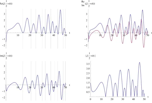
axis. This is represented in Figure 1. (calculated with “Mathematica 6” such as the further figures too). We see that not all of the zeros of the real part Re 1 i

2 t ζ

  ₊   _ _   are also zeros of the imaginary part Im 1 i

2 t ζ

  ₊   _ _

  and, vice versa, that not all of the zeros of the imaginary part are also zeros of the real part and thus genuine zeros of the function 1 i

2 t ζ_ + _

  which are signified by grid lines. Between two zeros of the real part which are genuine zeros of 1 i

2 t ζ_ + _

[image:10.595.48.548.308.645.2]

  lies in each case (exception first interval) an additional zero of the imaginary part, which almost coincides with a maximum of the real part.

Figure 1. Real and imaginary part and absolute value of Riemann zeta function on critical line. The position of the zeros of the whole function 1 i

2 t

ζ _ + _

  on the critical line are shown by grid lines. One can see that not all zeros of the real part are also zeros of the

982

Using (2.9) and definition (2.16) we find the following representation of Ξ

( )

z

( )

2

(

2 2

)

1

1

1 1

d exp π .

2 4

z z

n

q q

z z q n q

q

− ∞ +∞

=

+

 

Ξ = −_ − _ −

 

∫

∑

(2.23)

With the substitution of the integration variable q=eu (see also (2.10) in Appendix

A) representation (2.23) is transformed to

( )

2

( )

₂

(

2 2

)

0

1

1 1

2 d ch e exp π e .

2 4

u

u

n

z z u uz n

∞ +∞

=

 

Ξ ≡ − _ − _ −

 

∫

∑

(2.24)

In Appendix A we show that (2.24) can be represented as follows (see also Equation (2.2) on p. 17 in [5] which possesses a similar principal form)

( )

z ₀+∞du

( ) ( )

u ch uz ,

Ξ =

_∫

Ω (2.25) with the following explicit form of the function Ω

( )

u of the real variable u

( )

2 2 2

(

2 2

) (

2 2

)

1

4e π e 2π e 3 exp π e 0, ( ).

u

u u u

n

u n n n u

∞

=

Ω ≡

∑

− − > −∞ < < +∞ (2.26)

The function Ω

( )

u is symmetric

( )

u

( )

u

( )

u ,

Ω = +Ω − = Ω (2.27)

that means it is an even function although this is not immediately seen from representation (2.26)3_{. We prove this in Appendix A. Due to this symmetry, formula} (2.25) can be also represented by

( )

1

( ) ( )

1

( )

d ch d e .

2 2

uz

z +∞ u u uz +∞ u u

−∞ −∞

Ξ =

_∫

Ω =

_∫

Ω (2.28)

In the formulation of the right-hand side the function Ξ

( )

z appears as analytic

continuation of the Fourier transform of the function Ω

( )

u written with imaginary

argument z=iy or, more generally, with substitution z→iz′ and complex z′.

From this follows as inversion of the integral transformation (2.28) using (2.27)

( )

1

( )

i 1

( ) ( )

d i e d i cos ,

π

uy

u y y y y uy

π

+∞ ₋ +∞

−∞ −∞

Ω =

_∫

Ξ =

_∫

Ξ _(2.29)

or due to symmetry of the integrand in analogy to (2.25)

( )

2 ₀

( ) ( )

d i cos ,

π

u +∞ y y uy

Ω =

_∫

Ξ _(2.30)

where Ξ

( )

iy is a real-valued function of the variable y on the imaginary axis

( )

( ) ( )

(

( )

)

*

( )

0

iy +∞du u cos uy , iy iy ,

Ξ =

_∫

Ω Ξ = Ξ _(2.31)

due to (2.25).

A graphical representation of the function Ω

( )

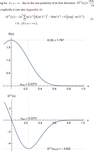
u and of its first derivatives

3_{It was for us for the first time and was very surprising to meet a function where its symmetry was not easily}

seen from its explicit representation. However, if we substitute in (2.26) u→ −u and calculate and plot the

( )1

_{( ) (}

₎

, 1, 2, 3

u n

Ω = is given in Figure 2. The function Ω

( )

u is monotonically de-

creasing for 0≤ < +∞u due to the non-positivity of its first derivative ( )1

( )

u

( )

u u

∂Ω

Ω ≡

∂ which explicitly is (see also Appendix A)

( )

_{( )}

(

(

)

)

(

)

(

)

2

1 2 2 2 2 2 2 2 2 2

1

2e π e 8 π e 30π e 15 exp π e

0, 0 ,

u

u u u u

n

u n n n n

u

∞

=

Ω = − − + −

≤ ≤ < +∞

[image:12.595.215.541.91.622.2]

∑

_(2.32)

Figure 2. Function Ω

( )

u and its first derivative Ω( )1

( )

u (see (2.25) and (2.34)).

The function Ω

( )

u is positive for 0≤ < +∞u and since its first derivative

( )1

_{( )}

u

Ω is negative for 0< < +∞u the function Ω

( )

u is mono- tonically

with one relative minimum at umin =0.237266 of depth

( )1

₍

₎

min 4.92176

u

Ω = − .

Moreover, it is very important for the following that due to presence of factors

(

2 2

)

exp −π en u in the sum terms in (2.26) or in (2.32) the functions Ω

( )

u and ( )1

_{( )}

u

Ω _{and all their higher derivatives are very rapidly decreasing for} u→ +∞, more

rapidly than any exponential function with a polynomial of u in the argument. In this

sense the function Ω

( )

u is more comparable with functions of finite support which

vanish from a certain u≥u0 on than with any exponentially decreasing function.

From (2.27) follows immediately that the function ( )1

( )

u

Ω _{is antisymmetric}

( )1

_{( )}

( )1

_{( )}

_{( )}

( )1

_{( )}

, 0 0,

u

u u u

u u

∂

Ω = −Ω − = Ω ⇒ Ω =

∂ (2.33)

that means it is an odd function.

It is known that smoothness and rapidness of decreasing in infinity of a function change their role in Fourier transformations. As the Fourier transform of the smooth (infinitely continuously differentiable) function Ω

( )

u the Xi function on the critical

line Ξ

( )

iy is rapidly decreasing in infinity. Therefore it is not easy to represent the

real-valued function Ξ

( )

iy with its rapid oscillations under the envelope of rapid

decrease for increasing variable y graphically in a large region of this variable y. An

appropriate real amplification envelope is seen from (2.18) to be

( )

1 4

2

1 2π

1 i2 _{1 4}

! 4

y

y _y

α =

+

  ₊

 

 

which rises Ξ

( )

iy to the level of the Riemann zeta

function 1 i 2 t ζ_ + _

  on the critical line z=iy. This is shown in Figure 3. The partial picture for α

( ) ( )

y Ξ iy in Figure 3. with negative part folded up is identical with the

absolute value 1 i 2 t ζ_ + _

  of the Riemann zeta function ζ

( )

s on the imaginary axis 1

i 2

s= + t (fourth partial picture in Figure 1).

We now give a representation of the Xi function by the derivative of the Omega function. Using ch

( )

uz 1 sh

( )

uz

z u

∂ =

∂ one obtains from (2.25) by partial integration the following alternative representation of the function Ξ

( )

z

( )

( )1

_{( ) ( )}

0

1

d sh ,

z u u uz

z

+∞

Ξ = −

_∫

Ω (2.34) that due to antisymmetry of ( )1

( )

u

Ω _and sh

( )

uz with respect to u→ −u can also

be written

( )

1 ( )1

_{( ) ( )}

1 ( )1

_{( )}

= d sh = d e .

2 2

uz

z u u uz u u

z z

+∞ +∞

−∞ −∞

[image:13.595.189.554.340.727.2]

Ξ −

_∫

Ω −

_∫

Ω _(2.35)

Figure 2 gives a graphical representation of the function Ω

( )

u and of its first

derivative ( )1

( )

( )

u u

u

∂Ω

Ω ≡

[image:14.595.48.554.64.391.2]

Figure 3. Xi Function Ξ

( )

iy on the imaginary axis z=iy (corresponding to 1 i 2

s= + y). The envelope over the oscillations of the

real-valued function Ξ

( )

iy decreases extremely rapidly with increase of the variable y in the shown intervals. This behavior makes it

difficult to represent this function graphically for large intervals of the variable y. By an enhancement factor which rises the amplitude to

the level of the zeta function ζ

( )

s we may see the oscillations under the envelope (last partial picture). A similar picture one obtains for

the modulus of the Riemann zeta function 1 i

2 y

ζ_ + _

  only with our negative parts folded to the positive side of the ordinate, i.e.

( )

1

i i

2

y ζ y

Ξ = _ + _

  (see also Figure 1 (last partial picture)). The given values for the zeros at 1

i

2± yn were first calculated by J.-P.

Gram in 1903 up to y15 [5]. We emphasize here that the shown very rapid decrease of the Xi function at the beginning of y and for

y→ ±∞ is due to the “very high” smoothness of Ω

( )

u for arbitrary u.

generate by computer. One can express Ξ

( )

z also by higher derivatives

( )n

_{( )}

n

_{( )}

n

u u

u

∂ Ω

Ω ≡

∂ of the Omega function Ω

( )

u according to

( )

( )

_{( ) ( )}

( )

_{( ) ( ) (}

₎

2 2 0

2 1 2 1 0

1

d ch

1

d sh , 0,1, 2, ,

m m

m m

z u u uz

z

u u uz m

z

+∞

+∞ ₊

+

Ξ = Ω

= − Ω =

∫

∫



(2.36)

with the symmetries of the derivatives of the function Ω

( )

u for u↔ −u

( )2

_{( )}

( )2

_{( )}

(2 1)

_{( )}

(2 1)

_{( )}

(2 1)

_{( )}

₍

₎

, , 0 0, 0,1, .

m m m m m

u u + u + u + m

This can be seen by successive partial integrations in (2.25) together with complete induction. The functions ( )n

( )

u

Ω _{in these integral transformations are for} n≥1 not monotonic functions.

We mention yet another representation of the function Ξ

( )

z . Using the trans-

formations

2 2 2 2

π e , u d 2π e du 2 d ,

n n n

t ≡ n ⇒ t = n u= t u (2.38)

the function Ξ

( )

z according to (2.28) with the explicit representation of the function

( )

u

Ω _{in (2.26) can now be represented in the form}

( )

( )

( )

( )

( )

( )

2 2 2 2

1 1 2 4

2 2 2 2

1 9 9

2 π 2 ,π π 2 ,π

4 2 4 2

π

5 5

3 π 2 ,π π 2 ,π ,

4 2 4 2

z z

n

z z

z z

z n n n n

n

z z

n n n n

∞ ₋

=

−

  

    

Ξ = _{ } Γ_ + _+ Γ_ − _

   

  





 _{   }

−  Γ_ + _+ Γ_ − 

 

 

∑

(2.39)

where Γ ,

( )

α x denotes the incomplete Gamma function defined by (e.g., [18] [21]

[36])

(

)

1

( ) (

)

, d et , .

x

x t tα x

α +∞ − − α γ α

Γ ≡

_∫

≡ Γ − (2.40)

However, we did not see a way to prove the Riemann hypothesis via the repre- sentation (2.39).

The Riemann hypothesis for the zeta function ζ

(

s= +σ it

)

is now equivalent to

the hypothesis that all zeros of the related entire function Ξ = +

(

z x iy

)

lie on the

imaginary axis z=iy that means on the line to real part x=0 of z= +x iy which

becomes now the critical line. Since the zeta function

ζ

(

s

)

does not possess zeros in the convergence region σ >1 of the Euler product (2.1) and due to symmetries (2.27) and (2.31) it is only necessary to prove that Ξ

( )

z does not possess zeros within the

strips 1 0 2 x

− ≤ < and 0 1

2

x

< ≤ + to both sides of the imaginary axis z=iy where

for symmetry the proof for one of these strips would be already sufficient. However, we will go another way where the restriction to these strips does not play a role for the proof.

3. Application of Second Mean-Value Theorem of Calculus to Xi

Function

After having accepted the basic integral representation (2.25) of the entire function

( )

z

Ξ according to

( )

z ₀+∞du

( ) ( )

u ch uz ,

Ξ ≡

_∫

Ω _(3.1) with the function Ω

( )

u explicitly given in (2.26) we concentrate us on its further

treatment. However, we do this not with this specialization for the real-valued function

( )

u

Ω _{but with more general suppositions for it. Expressed by real part} U x y

( )

, and

(

)

( )

( )

( )

(

( )

)

*

( )

(

( )

)

*

i , i , , , , , , , ,

x y U x y V x y U x y U x y V x y V x y

Ξ + ≡ + = = _(3.2)

we find from (3.1)

( )

, ₀ d

( ) ( ) ( )

ch cos ,

( )

, ₀ d

( ) ( ) ( )

sh sin .

U x y =

∫

+∞ uΩ u ux uy V x y =

∫

+∞ uΩ u ux uy (3.3)

We suppose now as necessary requirement for Ω

( )

u and satisfied in the special

case (2.26)

( )

u 0, 0

(

u

)

,

( )

0 0.

Ω > ≤ < +∞ ⇒ Ω > _(3.4) Furthermore, Ξ

( )

z should be an entire function that requires that the integral (3.1)

is finite for arbitrary complex z and therefore that Ω

( )

u is rapidly decreasing in

infinity, more precisely

( )

(

)

lim 0, 0 0 ,

exp

u

u

u λ

λ

→∞

Ω

= < ≤ < +∞

− (3.5)

for arbitrary λ ≥0. This means that the function Ω

( )

u should be a nonsingular

function which is rapidly decreasing in infinity, more rapidly than any exponential function e−λu _{with arbitrary}

0

λ > _{. Clearly, this is satisfied for the special function}

( )

u

Ω _{in (2.26).}

Our conjecture for a longer time was that all zeros of Ξ

( )

z lie on the imaginary

axis z=iy for a large class of functions Ω

( )

u and that this is not very specific for

the special function Ω

( )

u given in (2.26) but is true for a much larger class. It seems

that to this class belong all non-increasing functions Ω

( )

u , i.e such functions for

which holds ( )1

( )

0

u

Ω ≤ _{for its first derivative and which rapidly decrease in infinity.} This means that they vanish more rapidly in infinity than any power functions

(

)

, 1, 2, n

u− n=  (practically they vanish exponentially). However, for the conver-

gence of the integral (3.1) in the whole complex z-plane it is necessary that the

functions have to decrease in infinity also more rapidly than any exponential function

(

)

exp −λu with arbitrary λ >0 expressed in (3.5). In particular, to this class belong all rapidly decreasing functions Ω

( )

u which vanish from a certain u≥u₀ on and

which may be called non-increasing finite functions (or functions with compact support). On the other side, continuity of its derivatives Ω( )n

( ) (

u , n=1, 2,

)

is not required. The modified Bessel functions I_ν

( )

z “normalized” to the form of entire

functions 2 I

( )

z z

ν

ν

   

  for 1 2

ν ≥ possess a representation of the form (3.1) with functions Ω

( )

u which vanish from u≥1 on but a number of derivatives of Ω

( )

u

for the functions is not continuous at u=1 depending on the index ν . It is valuable that here an independent proof of the property that all zeros of the modified Bessel functions I_ν

( )

u lie on the imaginary axis can be made using their differential eq-

uations via duality relations. We intend to present this in detail in a later work.

( )

u

Ω _{cannot stay on the same level in a certain interval that means we have}

( )1

_{( )}

0

u

Ω < _{for all points} u>0 instead of Ω( )1

( )

u ≤0 only. A function which de- creases not faster than e−λu in infinity does not fall into this category as, for example, the function sech

( )

1

_{( )}

ch

z

z

≡ _shows.

To apply the second mean-value theorem it is necessary to restrict us to a class of functions Ω

( )

u → f u

( )

which are non-increasing that means for which for all

1 2

u <u in considered interval holds

( )

( )

1

( )

2

( )

0,

(

1 2

)

,

f a ≥ f u ≥ f u ≥ f b ≥ a≤ ≤u u ≤b (3.6)

or equivalently in more compact form

( )1

_{( )}

₍

₎

0, .

f u ≤ a≤ ≤u b (3.7)

The monotonically decreasing functions in the interval a≤ ≤u b, in particular,

belong to the class of non-increasing functions with the fine difference that here

( )

( )

1

( )

2

( )

0,

(

1 2

)

,

f a > f u > f u > f b > a< <u u <b (3.8)

is satisfied. Thus smoothness of f u

( )

for a< <u b is not required. If furthermore

( )

g u is a continuous function in the interval a≤ ≤u b the second mean-value

theorem (often called theorem of Bonnet (1867) or Gauss-Bonnet theorem) states an equivalence for the following integral on the left-hand side to the expression on the right-hand side according to (see some monographs about Calculus or Real Analysis; we recommend the monographs of Courant [37] (Appendix to chap IV) and of Widder [38] who called it Weierstrass form of Bonnet’s theorem (chap. 5, §4))

( ) ( )

( )

0

( )

( )

( ) (

)

0 0

d d d , ,

b u b

a u f u g u = f a a ug u + f b u ug u a≤u ≤b

∫

∫

∫

(3.9)

where u0 is a certain value within the interval boundaries a<b which as a rule we

do not exactly know. It holds also for non-decreasing functions which include the monotonically increasing functions as special class in analogous way. The proof of the second mean-value theorem is comparatively simple by applying a substitution in the (first) mean-value theorem of integral calculus [37][38].

Applied to our function f u

( )

= Ω

( )

u which in addition should rapidly decrease in

infinity according to (3.5) this means in connection with monotonic decrease that it has to be positively semi-definite if Ω

( )

0 >0 and therefore

( )

( )

( )1

_{( )}

₍

₎

₍

₎

0 u 0, u 0, 0 u , u 0,

Ω ≥ Ω ≥ Ω ≤ ≤ ≤ +∞ Ω → +∞ → (3.10)

and the theorem (3.9) takes on the form

( ) ( )

( )

0

( ) (

)

0

0 d 0 0 d , 0 ,

u

u u g u ug u u

+∞

Ω = Ω ≤ < +∞

∫

∫

(3.11)

where the extension to an upper boundary b→ +∞ in (3.9) for f

( )

+∞ =0 and in

case of existence of the integral is unproblematic.

If we insert in (3.9) for g u

( )

the function ch

( )

uz which apart from the real

variable u depends in parametrical way on the complex variable z and is an analytic

way as follows

( )

( ) ( )

( )

0( )

( )

( )

(

0

( )

)

( )

( )

( )

0 0 0

0 0

sh

d ch 0 w zd ch 0 w z z , , i , ,

z u u uz u uz w z u x y v x y

z

+∞

Ξ ≡

_∫

Ω = Ω

_∫

= Ω = + _(3.12)

where w x0

(

+iz

)

=u0

( )

x y, +iv x y0

( )

, is an entire function with u0

( )

x y, its real and

( )

0 ,

v x y its imaginary part. The condition for zeros z≠0 is that sh

(

w0

( )

z z

)

vanishes that leads to

( )

(

( )

( )

)

(

)

(

)

0 0 , i 0 , i i π, 0, 1, 2, ,

w z z= u x y + v x y x+ y = n n= ± ±  (3.13)

or split in real and imaginary part

( )

( )

0 , 0 , 0,

u x y x v− x y y= (3.14)

for the real part and

( )

( )

(

)

0 , 0 , π, 0, 1, 2, ,

u x y y v x y x+ =n n= ± ±  (3.15)

for the imaginary part.

The multi-valuedness of the mean-value functions in the conditions (3.13) or (3.15) is an interesting phenomenon which is connected with the periodicity of the function

( )

ch

( )

g u = uz on the imaginary axis z=iy in our application (3.12) of the second

mean-value theorem (3.11). To our knowledge this is up to now not well studied. We come back to this in the next Sections 4 and, in particular, Section 7 brings some illustrative clarity when we represent the mean-value functions graphically. At present we will say only that we can choose an arbitrary n in (3.15) which provides us the

whole spectrum of zeros z z1, 2, on the upper half-plane and the corresponding

spectrum of zeros z−1= −z z1, −2= −z2, on the lower half-plane of  which as will

be later seen lie all on the imaginary axis. Since in computer calculations the values of the Arcus Sine function are provided in the region from π

2

− _to π 2

+ _{it is convenient} to choose n=0 but all other values of n in (3.15) lead to equivalent results.

One may represent the conditions (3.14) and (3.15) also in the following equivalent form

( )

( )

0 , 2 2 π, 0 , 2 2 π,

y x

u x y n v x y n

x y x y

= =

+ + (3.16)

from which follows

( )

( )

(

2 2

)(

2 2

)

( )

2 0

( )

_{( )}

0 0

0

,

, , π , .

,

v x y x u x y v x y x y n

u x y y

+ + = = _(3.17)

All these forms (3.14)-(3.17) are implicit equations with two variables

( )

x y, which

cannot be resolved with respect to one variable (e.g., in forms y= yk

( )

x for each

fixed n and branches k) and do not provide immediately the necessary conditions

for zeros in explicit form but we can check that (3.16) satisfies the Cauchy-Riemann equations as a minimum requirement

( )

( )

( )

( )

0 , 0 , 0 , 0 ,

, .

u x y v x y u x y v x y

x y y x

∂ ∂ ∂ ∂

= = −

We have to establish now closer relations between real and imaginary part u0

( )

x y,

and v0

( )

x y, of the complex mean-value parameter w z0

(

= +x iy

)

. The first step in

preparation to this aim is the consideration of the derived conditions on the imaginary axis.

4. Specialization of Second Mean-Value Theorem to Xi Function

on Imaginary Axis

By restriction to the real axis y=0 we find from (3.3) for the function Ξ

( )

z

( )

x U x

( )

, 0 , V x

( )

, 0 0,

Ξ = = _(4.1)

with the following two possible representations of U x

( )

, 0 related by partial in-

tegration

( )

( ) ( )

( )1

_{( ) ( )}

0 0

1

, 0 d ch d sh 0.

U x u u ux u u ux

x

+∞ +∞

=

_∫

Ω = −

_∫

Ω > _(4.2)

The inequality U x

( )

, 0 >0 follows according to the supposition Ω

( )

u ≥ Ω0,

( )

0 >0

from the non-negativity of the integrand that means from Ω

( ) ( )

u ch ux ≥0. Therefore,

the case y=0 can be excluded from the beginning in the further considerations for zeros of U x y

( )

, and V x y

( )

, .

We now restrict us to the imaginary axis x=0 and find from (3.3) for the function

( )

z

Ξ

( )

iy U

( )

0,y , V

( )

0,y 0.

Ξ = = (4.3)

with the following two possible representations of U

( )

0,y related by partial in-

tegration

( )

( ) ( )

( )1

_{( ) ( )}

0 0

1

0, d cos d sin .

U y u u uy u u uy

y

+∞ +∞

=

_∫

Ω = −

_∫

Ω _(4.4)

From the obvious inequality

( )

1 cos uy 1,

− ≤ ≤ + _(4.5) together with the supposed positivity of Ω

( )

u one derives from the first repre-

sentation of U

( )

0,y in (4) the inequality

( )

( )

( )

0 U 0,y 0, 0 U 0, 0 ₀ du u 0. +∞

−Ω ≤ ≤ +Ω Ω = ≡

_∫

Ω ≥ (4.6)

In the same way by the inequality

( )

1 sin uy 1,

− ≤ ≤ + _(4.7) one derives using the non-positivity of ( )1

( )

u

Ω _{(see (3.10)) together with the second} representation of U

( )

0,y in (4.4) the inequality

( )

( )

( ) ( )

( )1

_{( )}

0

0 U 0,y y 0 , 0 +∞du u 0.

−Ω ≤ ≤ +Ω Ω = −

_∫

Ω ≥ _(4.8)

which as it is easily seen does not depend on the sign of y. Therefore we have two

according to (4.6) and (4.8) restrict the range of values of U

( )

0,y to an interior range

both to (4.6) and to (4.8) at once.

For mentioned purpose we now consider the restriction of the mean-value parameter

( )

0

w z to the imaginary axis z=iy for which g u

( )

=ch

(

u y

( )

i

)

=cos

( )

uy is a real-

valued function of y. For arbitrary fixed y we find by the second mean-value

theorem a parameter u0 in the interval 0≤ < +∞y which naturally depends on the

chosen value y that means u0 =u0

( )

0,y . The extension from the imaginary axis

i

z= y to the whole complex plane  can be made then using methods of complex

analysis. We discuss some formal approaches to this in Appendix B. Now we apply (3.12) to the imaginary axis z=iy.

The second mean-value theorem (3.12) on the imaginary axis z=iy (or x=0) takes on the form

( )

(

( )

)

( ) ( )

( )

( )

( )

( )

(

( )

)

(

( )

( )

)

0, 0

0 0 0

0

0 0

d ch i d cos 0 d cos

sin 0,

0 , 0, 0, 0, 0 .

u y

u u u y u u uy u uy

u y y

u y v y

y

+∞ +∞

Ω = Ω = Ω

= Ω ≠ =

∫

∫

∫

(4.9)

As already said since the left-hand side is a real-valued function the right-hand side has also to be real-valued and the parameter function w0

( )

iy is real-valued and there-

fore it can only be the real part u0

( )

0,y of the complex function

(

)

( )

( )

0 i 0 , i 0 ,

w z= +x y =u x y + v x y for x=0.

The second mean-value theorem states that u0

( )

0,y lies between the minimal and

maximal values of the integration borders that is here between 0 and +∞ and this means that u0

( )

0,y should be positive. Here arises a problem which is connected

with the periodicity of the function g u

( )

=cos

( )

uy as function of the variable u for

fixed variable y in the application of the mean-value theorem. Let us first consider

the special case y=0 in (4.9) which leads to

( )

( )

0

( )

( )

( )

0

( )

0 0 0 0

0 0 0

0 1

sin

d 0 ud 0 0 lim , 0, 0 0.

y

u y

u u u u u u u

u y

+∞

→

=

Ω = Ω = Ω = Ω ≡ >

∫

∫



(4.10)

From this relation follows u0≡u0

( )

0, 0 >0 and it seems that all is correct also with

the continuation to u0

( )

0,y >0 for arbitrary y. One may even give the approximate

values Ω

( )

0 ≈1.78679 and u₀ ≈0.27822 and therefore Ω ≡ Ω0

( )

0 u0≈0.49712

which, however, are not of importance for the later proofs. If we now start from

( )

0 0, 0 0

u > and continue it continuously to u₀

( )

0,y then we see that u₀

( )

0,y

goes monotonically to zero and approaches zero approximately at y= y1≈14.135

that is at the first zero of the function Ξ

( )

iy on the positive imaginary axis and goes

then first beyond zero and oscillates then with decreasing amplitude for increasing y

around the value zero with intersecting it exactly at the zeros of Ξ

( )

iy . We try to

illustrate this graphically in Section 7. All zeros lie then on the branch u0

( )

0,y y=nπ

with n=0. That u0

( )

0,y goes beyond zero seems to contradict the content of the