Munich Personal RePEc Archive
International RD Rivalry with a
Shipping Firm
Takauchi, Kazuhiro
Department of Economics, Management and Information Science,
Onomichi University
20 February 2012
Online at
https://mpra.ub.uni-muenchen.de/36843/
Current version: February 22, 2012
International R&D Rivalry with a Shipping Firm
Kazuhiro Takauchi
†Department of Economics, Management and Information Science
Onomichi University
Abstract
To examine the role of shipping firms in the international research and development (R&D) rivalry, we build a two-country (exporting and importing), two-firm (exporting and local) duopoly model with a shipping firm. The exporting firm competes with the local firm in the duopoly market of the local country but must pay a shipping fee to the shipping firm in order to sell its product in the local market. Similar to market competition, exporting and local firms engage in R&D competition. We compare two timing structures of the game: in one, the R&D stage is first, and in the other, the shipping firm is the leader. We show that when the R&D stage is first, there are ranges of parameter values such that the investment level of the exporting firm decreases as R&D becomes more efficient. When the shipping firm is the leader, we show that there are ranges of parameter values such that the profit of the local firm decreases as R&D becomes more efficient. Further, it is shown that consumers in the local country prefer the regime in which the shipping firm is the leader, whereas the government of the local country prefers the other regime.
JEL classification: F12; F13; L13
Keywords: International trade; R&D rivalry; Shipping firm
†
Corresponding author: Kazuhiro Takauchi
Department of Economics, Management, and Information Science, Onomichi University,
1600 Hisayamada, Onomichi, Hiroshima 722-8506, Japan. E-mail: takauch@onomichi-u.ac.jp
Fax: +81-078-803-6877
1
Introduction
Strategic research and development (R&D) investment has been widely discussed in the
liter-ature on international trade. Following the seminal work of Spencer and Brander (1983), for
example, Leahy and Neary (1996, 1999), Muniagurria and Singh (1997), Qiu and Tao (1998),
Dewit and Leahy (2004, 2011), Kujal and Ruiz (2007, 2009), and Takauchi (2011) focus on the
effects of R&D subsidy policy, the spillover effects of investment, trade liberalization effects on
firms’ investment strategy and welfare, and the interactions between other trade policies and
firms’ R&D incentives in oligopolistic markets.1
However, the literature ignores one important factor on international trade: the role of ship-ment.2 In fact, since producers and shippers are not necessarily the same, we must distinguish
between producers and shippers for more a realistic consideration of international
competi-tion with R&D.3 If a shipping fee is determined by a shipping firm, how is the international
R&D rivalry between exporting and domestic firms affected? In other words, compared with a
traditional result, does the nature of the output and the investment strategies of firms change?
To answer this question, in the present paper, we consider a model of international R&D
rivalry with a shipping firm. There are two producers, exporting and local firms, and a
non-producer, a shipping firm. Local and exporting firms compete `a la Cournot in the market of
the local country and engage in R&D activity, whereas the shipping firm carries the product
produced by the exporting firm from the exporting country to the market of the local country. In this situation, we examine two different timing games: in the first, the R&D investment level
is first chosen by the exporting and local firms; in the second, the shipping firm is the leader.
In cost-reducing R&D competition, it may be expected that if the efficiency of R&D improves
(or a cost parameter of R&D decreases), firms have larger incentives to invest, the volume of
R&D investment increases, and output and profit increase. Because the efficiency of R&D
directly affects the volumes of investment and output, it has an important role. However, we
found some paradoxical results when R&D is highly efficient. First, we show that when the
R&D stage is first, the volume of R&D investment of the exporting firm is inverted-U shaped
1
There are other topics on international R&D rivalry that focus on firm heterogeneity. Assuming the R&D investment level of firm has no effect on the rival’s output choice and introducing a distribution function of cost, Long et al. (2011) examine trade liberalization effects with and without free entry in an oligopoly model. Their non-strategic R&D model is similar to the study of Haaland and Kind (2008), which assumes that each firm simultaneously chooses both R&D investment and output. Furthermore, although they do not consider international competition, there are recent works that focus on cost heterogeneity. Ishida et al. (2011) examine the relationship between firms’ competitive position and initial cost differences among firms.
2
In international trade theory, there are studies that focus on transportation services. Francois and Wooton (2001) consider shipping industry in a general equilibrium setting. Andriamananjara (2004) examines the reduc-tion of trade barriers in a two-way oligopoly model with the shipping industry. However, these studies do not consider firms’ R&D activity.
3
for the efficiency of R&D: if R&D is highly efficient, the exporter’s investment level decreases as
the efficiency of R&D improves. The key to this result is that the shipping fee decreases as the
volume of the exporting firm’s investment decreases. For that reason, to reduce the shipping
fee, the exporting firm commits to a smaller level of investment. Since this commitment also
increases the rival’s investment level, the exporter’s investment level decreases when the rival
has extremely larger incentives to invest.
Second, we show that when the shipping firm is the leader, the local firm’s profit is inverted-U shaped for the efficiency of R&D: if R&D investment is highly efficient, the profit of the
local firm decreases as the efficiency of R&D improves. In this case, the local firm invests
excessively given its much smaller increase in output. Since an increase in expenditure level in
R&D dominates an increase in gains of investment, the local firm’s profit falls.
Third, we show that in the case that R&D investment level is first decided, the shipping
fee is always higher than in the other case. This is because in the case that fee-setting is first
decided, for fear of a disadvantage to the exporting firm, the shipping firm always offers a
relatively low fee. As a result, in the case that R&D investment level is first decided, the profit
of the exporting firm is smaller than in other case, but the local firm has a larger profit in this
case.
Last, we demonstrate that consumers in the local country prefer the case that the shipping
firm is the leader, whereas the government of the local country prefers the case that R&D
investment is first decided. Commitment to a smaller investment level gives a larger benefit
to the rival firm (the local firm), but this does not cover the losses in total outputs of two
manufacturing firms. Therefore, in the case that the shipping firm is the leader, total output is
relatively large, whereas the profit of local firm is relatively large in the other case.
The role of a shipping firm in an international oligopoly is inspired by the work of Lahiri
and Ono (1999). They examine how a traditional argument on optimal tariff policy can be
altered when the producer and seller differ. To an international oligopoly model, they introduce
a middleman, called as “seller,” and demonstrate that the optimal policy is an import subsidy (i.e., a negative tariff rate) if the seller is the leader. Also they found that the sign of the
optimal tariff rate depends on the shapes of production cost and market structures. Although
their focus is on the tariff policy, in view of the presence of a middleman, our study is related
to theirs, although R&D rivalry was not considered in their work.
Our study is also related to some works on labor unions with oligopolies (e.g., Calabuig and
Gonzalez-Maestre, 2002; Haucap and Wey, 2004; and Manasakis and Petrakis, 2009). In our
model, the shipping firm sets the fee in a manner similar to that employed in the above labor
union model. Manasakis and Petrakis (2004) consider a cost-reducing R&D rivalry with a labor
However, our model is crucially different from the above labor union model.4 In the above
studies, it is assumed that each firm has a union (i.e., a decentralized regime) or that all firms
have a common union (i.e., a centralized regime). In our R&D competition model with a
shipping firm, the only exporting firm must use the shipping firm and pays a fee. This point,
that “one firm has a middleman but the other does not,” is basically different from the above
unionized industry model.5
In the next section, we build a model and examine firms’ investment and output strategies. Section 3 compares outcomes and examines welfare implications. Section 4 concludes.
2
Model
We consider a two-country partial equilibrium trade model with a shipping firm. There are two
countries, local and foreign. The local country has a product market, but the foreign country
does not have. We call the foreign an “exporting” country. Three firms—an exporting firm, a local firm, and a shipping firm—exist in the world, and the exporting (resp. local) firm
locates in the exporting (resp. local) country. Exporting and local firms are manufacturers of a
product and compete `a la Cournot in the local country’s market. Since the local firm is local,
we assume that this firm supplies its product without a shipping fee. On the other hand, since
the exporting firm is located overseas, it must use the shipping firm in order to carry its product
to the local market across international borders. To transport the product, the exporting firm
must pay a shipping fee,f, to the shipping firm.
Before market competition, exporting and local firms engage in cost-reducing R&D
compe-tition without spillover. The unit production cost isc(>0), and is the same between exporting
and local firms. To reduce the initial unit cost, both manufacturing firms make cost-reducing investments. After investment, the unit cost becomesc−xi, wherexi is the investment level of
manufacturing firm i. Variables associated with the two manufacturing firms are subscripted
by i=E, L (exporting and local). We assume that the R&D cost function is linear-quadratic:
(γ/2)(xi)2, where γ is the efficiency of R&D and a positive constant.6 That is, a smaller γ
corresponds to a higher efficiency in R&D.
A representative consumers’ utility function in the local country is U =z+aQ−(1/2)Q2,
4
Although Calabuig and Gonzalez-Maestre (2002) and Haucap and Wey (2004) consider a unionized industry, they do not examine R&D rivalry. In addition, there are other works on the unionized industry model. Lommerud et al. (2003) discuss a firm’s choice between exporting and foreign direct investment (FDI) with a labor union in a two-way oligopoly model. However, they do not consider R&D activity.
5
Our model also differs from Manasakis and Petrakis (2009) on the following point. To examine cooperative R&D regimes (RJVs), they focus on the role of spillover effects of investment, but ignore the cost parameter of R&D. In contrast to Manasakis and Petrakis (2009), we focus on the role of the cost parameter of R&D, but do not consider the spillover effects of investment.
6
wherez is consumption of the numerare good andQis the total supply of both manufacturing
firms: Q=∑i=E,Lqi, whereqi is the supply of manufacturing firmi. Hence, the inverse market
demand in local country is p = a−Q, where p is the product price, a is a positive constant, and a > c. Thus, the profit of each producing firm,Πi, is given by
ΠE ≡[a−(qE +qL)−(c−xE)−f]qE −
γ 2(xE)
2, (1)
ΠL≡[a−(qE +qL)−(c−xL)]qL−γ
2(xL) 2
. (2)
The shipping firm makes a take-it-or-leave-it offer to the exporting firm, and decides the fee,
f. The profit of the shipping firm,πS, is given by
πS≡(f−f0)qE, (3)
wheref0 is the minimum price of shipment. For simplicity, we normalizef0 to zero.
To examine the strategic interaction between the shipping firm and the manufacturing firms,
we consider two scenarios on the timing structures of the game. In the first, manufacturing firms’
R&D stage is first, and in the other, the shipping firm’s fee-setting stage is first (i.e., the shipping
firm is the leader). In general, since investment decisions do not have the flexibility of other production decisions, it is plausible that the investment stage will take place in the first stage of
the game. On the other hand, the shipping firm is a different player from manufacturing firms.
For this reason, we must consider these two cases.
In Case 1, the following timing structure is considered. At stage 1, the exporting and local
firms independently and simultaneously choose a volume of R&D investment. At stage 2, the
shipping firm sets the shipping fee. At stage 3, the exporting and local firms compete `a la
Cournot in the local market.
In Case 2, the timing structure is as follows. At stage 1, the shipping firm sets shipping fee.
At stage 2, the exporting and local firms independently and simultaneously choose a volume of
R&D investment. At stage 3, the exporting and local firms compete `a la Cournot in the local market.
The game has perfect information. Therefore, we use the subgame perfect Nash equilibrium
as the equilibrium concept and solve the game using backward induction.
In the next subsection, we calculate the equilibrium outcomes in two timing structures and
2.1 Case 1: The R&D stage is first
Third stage. The sxporting and local firms compete `a la Cournot in the market of the local
country. Using (1) and (2), the FOC for the profit maximization of each firm is
Exporting firm: 0 =a−c−f −2qE −qL+xE,
Local firm: 0 =a−c−qE −2qL+xL.
The above equations yield the following outputs in the third stage:
qE(xE, xL, f) = 1
3(a−c−2f + 2xE−xL); qL(xE, xL, f) = 1
3(a−c+f−xE+ 2xL). (4)
Second stage. In the second stage, the shipping firm chooses a level of the shipping fee f.
From (3) and (4), the FOC is
0 =−2 3f+
1
3(a−c−2f+ 2xE−xL).
Solving the above equation forf, we obtain the shipping fee in the second stage.
f(xE, xL) =
1
4(a−c+ 2xE −xL). (5)
Thus, fee rises (falls) as the volume of R&D investment of the exporting firm increases
(de-creases).
In the second stage, from (4) and (5), the outputs of exporting and local firms are
qE(xE, xL) =
1
6(a−c+ 2xE−xL); qL(xE, xL) = 1
12[5(a−c)−2xE+ 7xL]. (6)
First stage. Hereafter, we use “∗” as the symbol of the subgame perfect Nash equilibrium in Case 1 of the game. In the first stage, the exporting and local firms choose their respective
volumes of R&D investment. Using (1), (2), (5), and (6), FOCs in this R&D stage are
Exporting firm: 0 =a−c+ (2−9γ)xE−xL,
Local firm: 0 = 35(a−c)−14xE+ (49−72γ)xL.
The above equations yield the equilibrium levels of R&D investmentx∗
E andx
∗
The equilibrium output and profit of exporting and local firms are
q∗
E =
6(a−c)γ(6γ−7) 28−195γ+ 216γ2; q
∗
L=
6(a−c)γ(15γ−4)
28−195γ+ 216γ2, (7)
x∗
E =
4(a−c)(6γ−7) 28−195γ+ 216γ2; x
∗
L=
7(a−c)(15γ−4)
28−195γ+ 216γ2, and (8)
Π∗
E =
4(a−c)2(6γ−7)2γ(9γ−2) (28−195γ+ 216γ2)2 ; Π
∗
L=
(a−c)2(15γ−4)2γ(72γ−49)
2(28−195γ+ 216γ2)2 . (9)
The equilibrium shipping fee is
f∗
= 9(a−c)γ(6γ−7)
28−195γ+ 216γ2. (10)
From (3), (7), and (10), the equilibrium profit of the shipping firm is
π∗
S=
54(a−c)2γ2(6γ−7)2
(28−195γ+ 216γ2)2. (11)
Throughout the analysis, we make the following assumption.
Assumption 1 The efficiency of R&D is not too high, i.e., γ >4/3≃1.3333.
To ensure positive quantities for all outcomes in the two cases of the game, we require the above assumption. Note that this is a stronger condition on γ than the condition required to satisfy
the SOCs in both the R&D and fee-setting stages of the two timing structures.7 Thus, any
other conditions are satisfied as long as Assumption 1 holds.
Eqs. (7)–(9) yield the following proposition.
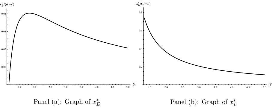
Proposition 1 In Case 1, (i) when R&D is highly efficient, the volume of R&D investment
of the exporting firm decreases as the efficiency of R&D improves; otherwise it increases as
the efficiency of R&D improves, i.e., ∂x∗
E/∂γ > 0 if γ < bγ ≡(1/12)(3 √
7 + 14) ≃1.8281 but
∂x∗
E/∂γ < 0 if γ >bγ. However, the volume of R&D investment of the local firm increases as
the efficiency of R&D improves. (ii) The output and profit of the exporting firm decrease, but
those of the local firm increase as the efficiency of R&D improves.
Proof. See Appendix A.
In a usual cost-reducing R&D competition, the volume of investment increases as R&D
improves (a decrease in the cost parameter of R&D).8 Thus, one might think that the result
shown in Proposition 1 is in sharp contrast to the intuition. When R&D is highly efficient, why
7
In case 1, the SOC for profit maximization in the R&D stage isγ >2/9≃0.22222 for the exporting firm
andγ >49/72≃0.680556 for the local firm.
8
1.5 2.0 2.5 3.0 3.5 4.0 4.5 5.0 Γ 0.01
0.02 0.03 0.04 xE*Ha-cL
Panel (a): Graph of x∗
E
1.5 2.0 2.5 3.0 3.5 4.0 4.5 5.0 Γ 0.2
0.4 0.6 0.8
xL*Ha-cL
Panel (b): Graph ofx∗
[image:9.595.73.527.82.263.2]L
Figure 1: Equilibrium investment level of both producing firms in Case 1
dose the exporting firm reduce the volume of investment as the efficiency of R&D improves?
The logic behind this result depends on two factors. The first is that the economy of scale
works in R&D investment; the effect is stronger if R&D is highly efficient. The second is that
to commit to a smaller level of investment reduces the shipping fee, which decreases as the
exporting firm’s investment level decreases.
In investment, each firm will invest heavily if it believes it can sell heavily. Furthermore,
since a smallerγ corresponds to a higher R&D efficiency, investment incentives are larger. The
exporting firm must pay the shipping fee, so it has a smaller market share than the local firm. That is, since the local firm has an advantage in market competition, the local firm invests
actively ifγ is sufficiently small.
The second factor promotes the effects of the scale economy. Since an investment level
is decided in the first stage of the game, the exporting firm can control the shipping fee. A
reduction in xE, from eq. (5), directly reduces the shipping fee and increases the rival’s
in-vestment level (i.e., strategic substitutes in the R&D stage). Additionally, from eq. (5), an
increase in the rival’s investment level also reduces the fee. To reduce the shipping fee, the
exporting firm always commits to a smaller level of investment; this behavior induces a larger
level of investment by the rival. When the efficiency of R&D is sufficiently high, the effects of
smaller investment extremely increase the rival’s investment and further reduces the investment level of the exporting firm. Therefore, ifγ becomes smaller than the critical level, bγ, then the
investment level of the exporting firm falls.
2.2 Case 2: The shipping firm is the leader
Second stage. In the second stage, each producing firm engages in R&D investment. Thus,
each firm’s FOC is as follows:9
Exporting firm: 0 = 1
9[4(a−c)−8f −(9γ−8)xE−4xL], Local firm: 0 = 1
9[4(a−c) + 4f −4xE −(9γ−8)xL].
Solving the above FOCs forxE andxL, we obtain the investment levels in the second stage.
xE(f) =
4[(a−c)(3γ−4)−2(3γ−2)f]
(3γ−4)(9γ−4) ; xL(f) =
4[(a−c)(3γ−4) + 3γf]
(3γ−4)(9γ−4) . (12)
From (12), the outputs of both producing firms in the second stage are
qE(f) =
3γ[(a−c)(3γ−4)−2(3γ−2)f]
(3γ−4)(9γ−4) ; qL(f) =
3γ[(a−c)(3γ−4) + 3γf]
(3γ−4)(9γ−4) . (13)
First stage. Hereafter, we use “∗∗” as the symbol of the subgame perfect Nash equilibrium in Case 2 of the game. The FOC for the shipping firm is
0 = 3γ[(a−c)(3γ−4)−4(3γ−2)f] (3γ−4)(9γ−4) .
Thus, solving the above FOC for f, we obtain the equilibrium shipping feef∗∗
in Case 2.10
f∗∗
= (a−c)(3γ−4)
4(3γ−2) . (14)
The equilibrium outcomes in Case 2 are
q∗∗
E =
3(a−c)γ 2(9γ−4); q
∗∗
L =
3(a−c)γ(15γ−8)
4(3γ−2)(9γ−4), (15)
x∗∗
E =
2(a−c) 9γ−4 ; x
∗∗
L =
(a−c)(15γ−8)
(3γ−2)(9γ−4), and (16)
Π∗∗
E =
(a−c)2γ(9γ−8) 4(9γ−4)2 ; Π
∗∗
L =
(a−c)2(15γ−8)2γ(9γ−8)
16(3γ−2)2(9γ−4)2 . (17)
The equilibrium profit of the shipping firm is
π∗∗
S =
3(a−c)2γ(3γ−4)
8(3γ−2)(9γ−4). (18)
9
The SOC for both producing firms in R&D stage isγ >8/9≃0.888889.
10
The SOC for the shipping firm is∂2
πS/∂f
2
=−12γ(3γ−2)/[(3γ−4)(9γ−4)]. Hence, the SOC holds as
Before the analysis on the outcomes of the two producing firms, let us compare the
equilib-rium shipping fees in the two cases. From (10), (11), (14), and (18), we establish the following
proposition.
Proposition 2 Regardless of the timing structures, (i) the shipping fee rises and becomes to
(1/4)(a−c) as the efficiency of R&D becomes worse;(ii)the profit of the shipping firm decreases
as the efficiency of R&D improves.
Proof. (i) Differentiating (10) and (14) with respect to γ, we obtain
∂f∗
∂γ =
18(a−c)(−98 + 168γ+ 171γ2) (28−195γ+ 216γ2)2 ,
∂f∗∗
∂γ =
3(a−c) 2(3γ−2)2 >0.
From the numerator of ∂f∗
/∂γ, −98 + 168γ + 171γ2 ≥ 0 for all γ ≥ (7/57)(3√6 −4) ≃ 0.411216. Hence, ∂f∗
/∂γ > 0. Further, rearranging (10) and (14), we find that limγ→∞f ∗
=
limγ→∞
(a−c)(54−(63/γ))
(28/γ2)−(195/γ)+216 = (1/4)(a−c) = limγ→∞f ∗∗
= limγ→∞
(a−c)(3−(4/γ)) 4(3−(2/γ)) . (ii) Differentiating (11) with respect toγ, we obtain
∂π∗
S
∂γ =
216(a−c)2γ(6γ−7)(−98 + 168γ+ 171γ2) (28−195γ+ 216γ2)3 ,
∂π∗∗
S
∂γ =
3(a−c)2(−16 + 24γ+ 9γ2) 4(3γ−2)2(9γ−4)2 .
From the above argument,∂π∗
S/∂γ >0. From the numerator of ∂π
∗∗
S /∂γ,−16 + 24γ+ 9γ2>0
for all γ >(4/3)(√2−1)≃0.552285. Q.E.D.
In our model, exporting and shipping firms have a certain “cooperative relationship.” Since
a shipping firm’s profit directly depends on the volume of output of the exporting firm, to ensure
positive production for the exporting firm, the shipping firm reduces its fee when the exporting
firm is extremely weak. Hence, the profit of shipping firm also goes down as the output of the
exporting firm goes down. This logic holds in both cases.
In a cost-reducing R&D competition, investment is not performed if the cost of R&D
in-creases indefinitely (i.e., xi → 0 as γ → ∞). That the shipping fee has an upper limit
corre-sponds to this fact.
From (15)–(17), we establish the following proposition.
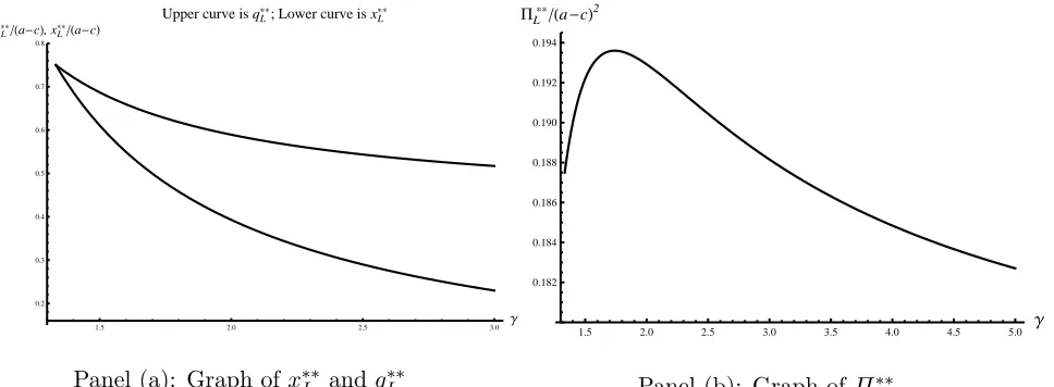
Proposition 3 In Case 2, (i) the output and volume of the R&D investment of local and
exporting firms increases as the efficiency of R&D improves. (ii)When R&D is highly efficient,
the profit of the local firm decreases as the efficiency of R&D improves; otherwise, it increases
as the efficiency of R&D improves, i.e., ∂Π∗∗
L/∂γ > 0 if γ < eγ ≃1.74008 but ∂Π
∗∗
L /∂γ <0 if
Proof. (i) Differentiating (15) with respect toγ, we obtain
∂q∗∗
E
∂γ =−
6(a−c) (9γ−4)2 <0,
∂q∗∗
L
∂γ =−
3(a−c)(32−120γ+ 117γ2)
(9γ−4)2 .
From the numerator of ∂q∗∗
L/∂γ, 32−120γ+ 117γ2 = 0 has no real root, and γ > 4/3 has a
positive value. Thus,∂q∗∗
L/∂γ <0. Differentiating (16) with respect to γ, we obtain
∂x∗∗
E
∂γ =−
18(a−c) (9γ−4)2 <0,
∂x∗∗
L
∂γ =−
3(a−c)(40−144γ+ 135γ2) (3γ−2)2(9γ−4)2 .
From the numerator of ∂x∗∗
L/∂γ, 40−144γ+ 135γ2 = 0 has no real root, and γ > 4/3 has a
positive value. Thus,∂x∗∗
L/∂γ <0.
(ii) Differentiating (17) with respect toγ, we obtain
∂Π∗∗
E
∂γ =
8(a−c)2 (9γ−4)3 >0,
∂Π∗∗
L
∂γ =−
(a−c)2(15γ−8)(−128 + 528γ−684γ2+ 243γ3)
4(3γ−2)3(9γ−4)3 .
From the numerator of ∂Π∗∗
L /∂γ, we find that −128 + 528γ −684γ2+ 243γ3 ≥0 forγ ≥eγ ≃
1.74008. Therefore,∂Π∗∗
L /∂γ ≤0 for γ ≥eγ and ∂Π
∗∗
L /∂γ >0 forγ <eγ. Q.E.D
1.5 2.0 2.5 3.0 Γ
0.2 0.3 0.4 0.5 0.6 0.7 0.8 qL**Ha-cL, xL**Ha-cL
Upper curve is q**L; Lower curve is xL**
Panel (a): Graph of x∗∗
L and q
∗∗
L
1.5 2.0 2.5 3.0 3.5 4.0 4.5 5.0 Γ
0.182 0.184 0.186 0.188 0.190 0.192 0.194 PL**Ha-cL2
Panel (b): Graph ofΠ∗∗
[image:12.595.63.547.422.600.2]L
Figure 2: Inverted-U shaped equilibrium profit of local firm
Panel (a) in Figure 2 shows that the local firm’s output and investment are decreasing with
γ. In Case 2, the shipping fee is decided in the first stage, so the exporting firm does not directly
control it. For this reason, the equilibrium investment and output levels of the two producing
firms have an ordinal nature with respect toγ, i.e.,∂q∗∗
i /∂γ <0 and∂x
∗∗
i /∂γ <0, fori=E, L.
inverted-U shaped for γ (see Panel (b)). That is, if R&D is highly efficient, the local firm’s
profit decreases as the efficiency of R&D improves.
Similar to Case 1 (Proposition 1), the local firm has a larger incentive to invest because the
local firm has an advantage in market competition. From (15) and (16), we find the following
relations in Case 2:
∆xq≡
∂x∗∗
L
∂γ
−
∂q∗∗
L
∂γ
=
9(a−c)[16 +γ(51γ−56)] 2(3γ−2)2(9γ−4)2 >0;
∂∆xq
∂γ <0.
Thus, the difference between an increase in investment and an increase in output expands when
R&D becomes more efficient.11
Why does this result occur? As shown in Proposition 2, the shipping fee falls as the efficiency
of R&D improves. For this reason, the cost difference between the exporting and local firms
closes as the efficiency of R&D improves. The effect of a closing cost difference induces an
increase in the output and profit of the exporting firm ((ii) of Proposition 3). Also, in Case 2,
the shipping fee is decided in the first stage of the game, so the exporting firm cannot commit
to a smaller level of investment to reduce the shipping fee. Thus, corresponding to an increase in output, the exporting firm increases its investment level if the efficiency of R&D improves.
The local firm suffers a loss from such behavior by the exporting firm. This is because the
local firm has an advantage in market competition from the beginning, but this advantage
becomes smaller when the shipping fee falls. Therefore, the local firm’s output increases, but
the increase in output is relatively smaller than the expenditure level of R&D. The effects of
excessive investment expand as the efficiency of R&D improves (∂∆xq/∂γ <0). Therefore, if
γ becomes smaller than the critical level, eγ, an increase in the expenditure level of investment
will dominate an increase in gains, and the profit of the local firm decreases.
3
Comparison among Outcomes/Welfare Implications
In this section, we compare welfares in Cases 1 and 2 and examine the relationship between
each country’s welfare and the efficiency of R&D.
Before the welfare analysis, let us compare the outcomes in Cases 1 and 2. From eqs.
(7)–(10) and (14)–(17), we establish the following proposition.
Proposition 4 Comparison between the outcomes in Case 1 (the R&D stage is first) and Case
2 (the shipping firm is the leader) yields
11
Formally, we obtain
∂∆xq
∂γ =−
9(a−c)(−256 + 1296γ−2268γ2+ 1377γ3)
(3γ−2)3(9γ−4)3
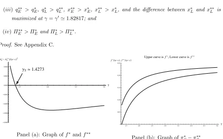
(i) f∗
> f∗∗ ;
(ii) π∗
S ≥π
∗∗
S if γ ≤γS and π
∗
S < π
∗∗
S if γ > γS, where γS≃1.4273;
(iii) q∗∗
E > q
∗
E, q
∗
L > q
∗∗
L, x
∗∗
E > x
∗
E, x
∗∗
L > x
∗
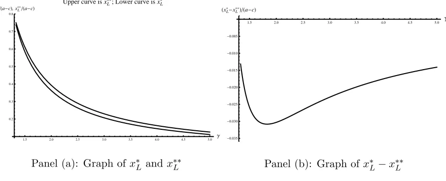
L, and the difference between x
∗
L and x
∗∗
L is
maximized at γ =γ′
≃1.82817; and
(iv) Π∗∗
E > Π
∗
E and Π
∗
L> Π
∗∗
L .
Proof. See Appendix C.
ΓS>1.4273
1.5 2.0 2.5 3.0 Γ
-0.008 -0.006 -0.004 -0.002 0.000 0.002 0.004 HΠS*- ΠS**LHa-cL2
Panel (a): Graph off∗
and f∗∗
1.5 2.0 2.5 3.0 3.5 4.0 4.5 5.0 Γ 0.05
0.10 0.15 0.20 0.25 f*Ha-cL, f**Ha-cL
Upper curve is f*; Lower curve is f**
Panel (b): Graph of π∗
S−π
∗∗
[image:14.595.76.528.114.397.2]S
Figure 3: Comparison f∗
and f∗∗ ;π∗
S and π
∗∗
S
Figures 3 and 4 depict investment levels in the local firm (claim (iii)), shipping fees, and
the difference in the profits of the shipping firm (claims (i) and (ii)). Claim (i) of Proposition
4 indicates that when the shipping fee can directly control the exporting firm’s investment
strategy, for fear of a disadvantage to the exporting firm, the shipping firm offers a relatively
lower fee. Thus, this is desirable for the exporting firm when the shipping firm is the leader, which corresponds to claim (iv), that is, Π∗∗
E > Π
∗
E.
Intuitively, from claim (i) of Proposition 4, one might think that the shipping firm has a
“second-mover advantage” in our model. However, in contrast to the result of the shipping fee,
the profit of the shipping firm is larger in Case 1 than in Case 2 if R&D is highly efficient. Claim
(ii) relies on claim (iii), that is, on the outputs ranking between the two cases: q∗∗
E > q
∗
E. Since
the exporting firm’s output is relatively small in Case 1 (although the shipping fee is relatively
high in that case), the profit of shipping firm is possibly larger in Case 1 than in Case 2.
Claim (iii) of Proposition 4 has an interesting result. This is because world total investment,
xE +xL, is larger in Case 2 than in Case 1. In particular, x∗∗L > x∗L is important. This result
corresponds to claim (ii) of Proposition 3, that is, the local firm invests excessively given its
1.5 2.0 2.5 3.0 3.5 4.0 4.5 5.0 Γ 0.2
0.3 0.4 0.5 0.6 0.7 0.8
xL*Ha-cL, xL**Ha-cL
Upper curve is xL**; Lower curve is xL*
Panel (a): Graph of x∗
L and x
∗∗
L
1.5 2.0 2.5 3.0 3.5 4.0 4.5 5.0 Γ
-0.035 -0.030 -0.025 -0.020 -0.015 -0.010 -0.005 HxL*-xL**LHa-cL
Panel (b): Graph of x∗
L−x
∗∗
[image:15.595.78.525.75.257.2]L
Figure 4: Comparisonx∗
L andx
∗∗
L
Claim (iv) is intuitive one. Since the profit of the producing firm depends on its output,
claim (iv) corresponds to the result of claim (iii). The exporting and local firms’ desirable
timing structures are opposite of one another.
Next, we consider welfare and consumer surplus in the local country. The social welfare
of the local country is given by WL ≡CS+ΠL, where consumer surplus is defined by CS =
(1/2)(qE+qL)2. Thus, welfare and consumer surplus in the two cases are
CS∗
= 18(a−c)
2γ2(21γ−11)2
(28−195γ+ 216γ2)2 , (19)
CS∗∗
= 81(a−c)
2γ2(7γ−4)2
32(3γ−2)2(9γ−4)2 , (20)
W∗
L=
(a−c)2γ(−784 + 11388γ−36297γ2+ 32076γ3)
2(28−195γ+ 216γ2)2 , (21)
W∗∗
L =
(a−c)2γ(−1024 + 6288γ−12456γ2+ 8019γ3)
32(3γ−2)2(9γ−4)2 . (22)
Consumer surplus and welfare in two cases increase as the efficiency of R&D improves:
∂CS/∂γ <0 and∂WL/∂γ <0 (see Appendix D).
Comparing (19) with (20), we obtain
CS∗
−CS∗∗
=−9(a−c)
2γ2(368−1056γ+ 729γ2)(−1040 + 6912γ−14103γ2+ 9072γ3) 32(3γ−2)2(9γ−4)2(28−195γ+ 216γ2)2 . (23)
Subsequently, comparing (21) with (22), we obtain
W∗
L−W
∗∗
L =
3(a−c)2γ2A
whereA≡523520−3860736γ+ 10300032γ2−11625120γ3+ 4221639γ4+ 629856γ5. From (23) and (24), we establish the following proposition.
Proposition 5 While consumers in the local country prefer the regime in which the shipping
firm is the leader, the government of the local country prefers the regime in which the R&D
stage is first.
Proof. From the right hand side of (23), 368−1056γ+729γ2 >0 for allγ >(4/243)(√73+44)≃
0.864922;−1040 + 6912γ−14103γ2+ 9072γ3 >0 for allγ >0.700737. Subsequently from the right hand side of (24), by numerical calculation, H > 0 for all γ > 0.695157. Therefore,
CS∗∗
> CS∗
andW∗
L> W
∗∗
L from Assumption 1. Q.E.D.
Proposition 5 implies that either the profit of the local firm or consumer surplus has the
larger effect on the welfare of local country. As shown in (iv) of Proposition 4, the local firm’s
profit is larger in Case 1 than in Case 2. However, from Proposition 5, consumer surplus (i.e.,
volume of total output) is larger in Case 2 than in Case 1. Since the national welfare of local
country is the sum of the local firm’s profit and consumer surplus, we find that a gain in the
profit of the local firm in Case 1 dominates a loss in consumer surplus in Case 2. In Case 1, to
reduce the shipping fee, the exporting firm commits to a smaller level of investment (Proposition 1). In Proposition 5, we can also verify that this commitment effect of the exporting firm gives
a larger benefit to the local firm.
Finally, we consider the social welfare of the exporting country. Hereafter, we assume that
the shipping firm is located in the exporting country. Then, the social welfare of the exporting
country, WE, is sum of the profits of the shipping and exporting firms, ΠE +πS. The social
welfare is given by
W∗
E =
2(a−c)2(6γ−7)2(45γ−4) (28−195γ+ 216γ2)2 ; W
∗∗
E =
(a−c)2γ(80−228γ+ 135γ2)
8(9γ−4)2(3γ−2) . (25)
In contrast to the welfare of the local country, the welfare of the exporting country decreases
as the efficiency of R&D improves: ∂WE/∂γ >0 (see Appendix D).
Eq. (25) yields the following result.
Corollary 1 Suppose that the shipping firm is located in the exporting country. Then, (i) the
social welfare of the exporting country is larger in Case 2 than in Case 1. (ii) The difference
between the social welfare of the exporting country in Cases 1 and 2 is maximized at γ =γ ≃
1.63951.
Proof. See Appendix C.
As shown in Proposition 4, the profit of the exporting firm is always larger in Case 2 than in
Case 1 than in Case 2. At first glance, welfare appears larger in Case 1 than in Case 2. However,
the welfare level in Case 2 dominates that in Case 1. Whereas the profit of the shipping firm
becomes smaller as the efficiency of R&D improves, the profit of the exporting firm in Case 2
increases as the efficiency of R&D improves. Therefore, the volume of the shipping firm’s profit
where R&D is sufficiently efficient is too small to reverse the ranking in the exporting firm’s
profit in Cases 1 and 2.
4
Conclusion
This paper builds a model of a two-country (exporting and local countries), two-firm
(export-ing and local firms) international R&D rivalry with a shipp(export-ing firm. Although R&D rivalry
has been broadly discussed in the literature of trade theory, the role of the shipping firm on
industrial competition has received little attention (e.g., Spencer and Brander, 1983; Leahy and
Neary, 1996, 1999; Muniagurria and Singh, 1997; Qiu and Tao, 1998; Dewit and Leahy, 2004, 2011; Kujal and Ruiz, 2007, 2009; Takauchi, 2011). To examine the interaction between the
endogenously decided shipping fee and the producing firm’s strategies, we consider different two
timing structures of the model. In one, the R&D investment level is first decided; in the other,
the shipping firm is the leader.
We have shown first that the exporting firm’s investment level is inverted-U shaped for the
efficiency of R&D when the R&D investment level is first decided in the game. That is, there
are ranges of parameter values such that the investment level goes down as the efficiency of
R&D improves. This is because the shipping fee decreases as the exporting firm’s investment
level decreases, and thus the exporting firm commits to a smaller investment level to reduce
the shipping fee. This behavior leads to an increase in the investment level of the rival firm. As a result, the exporting firm decreases its investment level when the rival firm has stronger
incentives to invest.
Second, we have shown that the local firm’s profit is inverted-U shaped for the efficiency
of R&D when the shipping firm is the leader. That is, there are ranges of parameter values
such that profit decreases as the efficiency of R&D improves. In this case, the local firm invests
excessively given its output. Since the loss in investment expenditure dominates the investment
gain, the profit of the local firm falls when R&D is highly efficient.
Third, we have shown that in the case that the R&D investment level is first decided,
the shipping fee is always higher than in the other case. For fear of a disadvantage to the
exporting firm, the shipping firm offers a relatively lower fee if it can control investment level of the exporting firm. For this reason, in the case that the R&D stage is first, the profit of the
exporting firm is smaller than in the other case, but local firm has a larger profit.
the shipping firm is the leader, wheres the government of local country prefers the regime in
which R&D stage is first. To commit to a smaller investment level gives a larger benefit to
the rival firm; this effect does not cover the losses in total output. Therefore, total output
is relatively large when the shipping firm is the leader, whereas the profit of the local firm is
relatively large when R&D stage is first.
In the cost-reducing R&D rivalry, the efficiency of R&D plays an important role. If the cost
of R&D improves, investment incentives and output increase. This undoubtedly increases profit of firms. However, our findings highlight some paradoxical results that occur if R&D is highly
efficient. Since all these findings depend on the behavior of the shipping firm, we believe that
our model developed herein offers new insight on international R&D competition.
2012/2/22 13:30
Acknowledgments
I thank Noriaki Matsushima for his many helpful comments. Of course, all errors are my own.
Appendix
A. Proof of Proposition 1
(i) Differentiating (8) with respect toγ, we obtain
∂x∗
E
∂γ =−
36(a−c)(133−336γ+ 144γ2) (28−195γ+ 216γ2)2 ,
∂x∗
L
∂γ =−
504(a−c)(5−24γ+ 45γ2) (28−195γ+ 216γ2)2 .
From the numerator of ∂x∗
E/∂γ, 133−336γ+ 144γ2 ≥ 0 for γ ≥(1/12)(3 √
7 + 14) ≃1.8281 and γ ≤(1/12)(−3√7 + 14)≃0.505229. This yields∂x∗
E/∂γ ≥0 if γ ≤(1/12)(3 √
7 + 14), but
∂x∗
E/∂γ <0 if γ > (1/12)(3 √
7 + 14). Subsequently, from the numerator of ∂x∗
L/∂γ, we find
that 5−24γ+ 45γ2 >0 for allγ. Thus, ∂x∗
L/∂γ <0.
(ii) Differentiating (7) with respect toγ, we obtain
∂q∗
E
∂γ =
12(a−c)(−98 + 168γ+ 171γ2) (28−195γ+ 216γ2)2 ,
∂q∗
L
∂γ =−
6(a−c)(112−840γ+ 2061γ2) (28−195γ+ 216γ2)2 .
From the numerator of ∂q∗
E/∂γ,−98 + 168γ+ 171γ2 >0 for γ >(7/57)(3 √
6−4)≃0.411216. Thus, ∂q∗
E/∂γ >0. Subsequently, from the numerator of ∂q
∗
L/∂γ, we find that 112−840γ+
2061γ2 = 0 has no real root and a positive value. Thus,∂q∗
Differentiating (9) with respect to γ, we obtain
∂Π∗
E
∂γ =
8(a−c)2(6γ−7)(196−903γ−342γ2+ 4374γ3)
(28−195γ+ 216γ2)3 ,
∂Π∗
L
∂γ =−
(a−c)2(15γ−4)(−5488 + 39648γ−137277γ2+ 138024γ3)
2(28−195γ+ 216γ2)3 .
From numerical calculation, we find that 196−903γ −342γ2+ 4374γ3 ≥ 0 for all γ ≥ γ2 ≃
−0.50553. Thus,∂Π∗
E/∂γ >0. Subsequently, from numerical calculation, we find that−5488 +
39648γ−137277γ2+ 138024γ3 >0 for all γ > γ3 ≃0.64468. Thus, ∂ΠL∗/∂γ <0. Q.E.D.
B. Proof of Proposition 4
(i) From (10) and (14), we obtain
f∗
−f∗∗
= (a−c)(261γ 2
−360γ+ 112) 4(3γ−2) (216γ2−195γ+ 28).
Since 261γ2−360γ+ 112>0 for allγ >(4/87)(√22 + 15)≃0.905306,f∗
> f∗∗ .
(ii) From (11) and (18), we obtain
π∗
S−π
∗∗
S = −
3(a−c)2γB
8(3γ−2)(9γ−4)(28−195γ2+ 216γ2)2,
whereB ≡ −3136−10416γ+ 75204γ2−107541γ3+ 42768γ4. By numerical calculation,B≤0 forγ ≤γS≃1.4273 but B >0 forγ > γS ≃1.4273.
(iii) From (7) and (15), we obtain
q∗
E−q
∗∗
E = −
9(a−c)γ(51γ−28) 2(9γ −4)(28−195γ+ 216γ2), q
∗
L−q
∗∗
L =
3(a−c)γ(−32−60γ+ 189γ2) 4(3γ−2)(9γ−4)(28−195γ+ 216γ2).
Thus,q∗∗
E > q
∗
E. Since−32−60γ+ 189γ2 >0 for allγ >(2/63)( √
193 + 5)≃0.59976, q∗
L> q
∗∗
L.
Subsequently, from (8) and (16), we obtain
x∗
E −x
∗∗
E =−
2(a−c)(−28−21γ+ 108γ2) (9γ−4)(28−195γ+ 216γ2).
Since−28−21γ+ 108γ2 >0 for allγ >(1/72)(√1393 + 7)≃0.615596,x∗∗
E > x
∗
E. Subsequently,
we obtain
x∗
L−x
∗∗
L =−
Since 100−249γ+ 135γ2 >0 for allγ >(1/90)(√889 + 83)≃1.25351, x∗∗
L > x
∗
L.
Subsequently, we have
∂(x∗
L−x
∗∗
L)
∂γ =
3(a−c)C
(3γ−2)2(9γ−4)2(28−195γ+ 216γ2)2,
where C ≡ −22400 + 111552γ + 145080γ2−1701000γ3+ 3549015γ4−2904336γ5+ 787320γ6. By numerical calculation,C= 0 for γ =γ≃1.82817.
(iv) From (9) and (17), we obtain
Π∗
E −Π
∗∗
E = −
3(a−c)2γD
4(9γ−4)2(28−195γ+ 216γ2)2,
whereD≡6272−58128γ+ 180432γ2−233685γ3+ 104976γ4. By numerical calculation,D >0 for all γ >1.00598. Thus,Π∗∗
E > Π
∗
E. Subsequently, we have
Π∗
L−Π
∗∗
L =
3(a−c)2γ2F
16(3γ−2)2(9γ−4)2(28−195γ+ 216γ2)2,
where F ≡ −312320 + 3532416γ−14720688γ2+ 29092608γ3−27680859γ4+ 10235160γ5. By numerical calculation,F >0 for allγ >0.569386. Thus, Π∗
L> Π
∗∗
L. Q.E.D.
C. Proof of Corollary 1
(i) From (25), the difference betweenW∗
E and W
∗∗
E yields
W∗
E−W
∗∗
E = −
3(a−c)2γG
8(3γ−2)(9γ−4)2(28−195γ+ 216γ2)2,
whereG≡ −12544 + 283584γ−1465056γ2+ 3124332γ3−2960955γ4+ 1014768γ5. By numerical calculation,G >0 for allγ >1.193. Thus, W∗∗
E > W
∗
E.
(ii) DifferentiatingW∗
E−W
∗∗
E with respect toγ, we obtain
∂(W∗
E−W
∗∗
E )
∂γ =
3(a−c)2H
4(3γ−2)2(9γ−4)3(28−195γ+ 216γ3)3,
whereH ≡1404928−50577408γ+402506496γ2−1160452224γ3+77639472γ4+7514537832γ5−
19546529013γ6 + 23059815480γ7−13281773472γ8+ 2959063488γ9.By numerical calculation, we find that H = 0 has one real root that satisfies Assumption 1, that is,H = 0 if and only if
D. The Effects of γ on Welfare
In view of welfare the intuitive results hold on the cost parameter of R&D. From (19)–(22), we
obtain the following.
∂CS∗
∂γ =−
36(a−c)2γ(21γ−11)(308−1176γ+ 1719γ2) (28−195γ+ 216γ2)3 .
Since 308−1176γ+ 1719γ2 = 0 has no real root and positive values,∂CS∗
/∂γ <0.
∂CS∗∗
∂γ =−
81(a−c)2γ(7γ−4)[16 +γ(51γ−56)] 8(3γ−2)3(9γ−4)3 <0, ∂W∗
L
∂γ =−
(a−c)2(21952−484848γ+ 2540916γ2−5750811γ3+ 4669488γ4)
2(28−195γ + 216γ2)3 .
By numerical calculation, since 21952−484848γ+ 2540916γ2−5750811γ3+ 4669488γ4 >0 for all γ >0.573553,∂W∗
L/∂γ <0.
∂W∗∗
L
∂γ =−
(a−c)2(2048−17472γ+ 54000γ2−72684γ3+ 36207γ4)
8(3γ−2)3(9γ−4)3 .
By numerical calculation, since 2048−17472γ + 54000γ2 −72684γ3 + 36207γ4 > 0 for all γ >0.617807,∂W∗∗
L /∂γ <0.
∂W∗
E
∂γ =
8(a−c)2(6γ−7)(196−3549γ+ 4194γ2+ 8991γ3)
(28−195γ+ 216γ2)3 ,
∂W∗∗
E
∂γ =
(a−c)2(320−1104γ+ 828γ2+ 243γ3) 4(3γ−2)2(9γ−4)3 ,
where 196−3549γ+4194γ2+8991γ3>0 for allγ >0.394337 and 320−1104γ+828γ2+243γ3>0 for all γ >−4.48568. Thus, ∂W∗
E/∂γ >0 and∂W
∗∗
E /∂γ >0.
References
[1] Andriamananjara, S., 2004. Trade and international transport services: An analytical frame-work. Journal of Economic Integration 19(3), 604–625.
[2] Calabuig, V., Gonzalez-Maestre, M., 2002. Union structure and incentives for innovation.
European Journal of Political Economy 18, 177–192.
[3] Dewit, G., Leahy, D., 2004. Rivalry in uncertain export markets: Commitment versus
[4] Dewit, G., Leahy, D., 2011. Strategic investment and gains from trade. NUIM Working
Papers N216-11.
[5] Francois, J., Wooton, I., 2001. Trade in international transport services: The role of
com-petition. Review of International Economics 9(2), 249–261.
[6] Haaland, J., Kind, H., 2008. R&D policies, trade and process innovation. Journal of
Inter-national Economics 74, 170–187.
[7] Haucap, J., Wey, C., 2004. Unionization structure and innovation incentives. Economic
Journal 114, 149–165.
[8] Ishida, J., Matsumura, T., Matsushima, N., 2011. Market competition, R&D and firm profits
in asymmetric oligopoly. Journal of Industrial Economics 59(3), 484–505.
[9] Kujal, P., Ruiz, J., 2007. Cost effectiveness of R&D and strategic trade policy. BE Journal
of Economic Analysis and Policy (Topics) 7, Article 21.
[10] Kujal, P., Ruiz, J., 2009. International trade policy towards monopoly and oligopoly.
Re-view of International Economics 17(3), 461–475.
[11] Lahiri, S., Ono, Y., 1999. Optimal tariffs in the presence of middlemen. Canadian Journal
of Economics 32, 55–70.
[12] Leahy, D., Neary, J.P., 1996. International R&D rivalry and industrial strategy without
government commitment. Review of International Economics 4(3), 322–338.
[13] Leahy, D., Neary, J.P., 1999. R&D spillovers and the case for industrial policy in an open
economy. Oxford Economic Papers 51, 40–59.
[14] Lommerud, K.E., Meland, F., Sorgard, L., 2003. Unionized oligopoly, trade liberalization
and location choice. Economic Journal 113, 782–800.
[15] Long, N.V., Raff, H., St¨ahler, F., 2011. Innovation and trade with heterogeneous firms.
Journal of International Economics 84(2), 149–159.
[16] Manasakis, C., Petrakis, E., 2009. Union structure and firms’ incentives for cooperative
R&D investments. Canadian Journal of Economics 42, 665–693.
[17] Motta, M., 2004. Competition policy: Theory and practice, Cambridge University Press,
Cambridge.
[18] Muniagurria, M.E., Singh, N., 1997. Foreign technology, spillovers, and R&D policy.
[19] Qiu, L.D., Tao, Z., 1998. Policy on international R&D cooperation: Subsidy or tax?.
European Economic Review 42, 1727–1750.
[20] Spencer, B.J., Brander, J.A., 1983. International R&D rivalry and industrial strategy.
Review of Economic Studies 50, 707–722.
[21] Takauchi, K., 2011. Rules of origin and international R&D rivalry. Economics Bulletin