Slip Suppression of Electric Vehicles Using Sliding Mode Control Method

http://dx.doi.org/10.4236/ica.2013.43038 Published Online August 2013 (http://www.scirp.org/journal/ica)

Slip Suppression of Electric Vehicles Using Sliding Mode

Control Method

*

Shaobo Li1, Tohru Kawabe2

1

Department of Computer Science, University of Tsukuba, Tsukuba, Japan

2

Faculty of Engineering, Information and Systems, University of Tsukuba, Tsukuba, Japan Email: [email protected], [email protected]

Received February 4, 2013; revised March 4, 2013; accepted March 11,2013

Copyright © 2013 Shaobo Li, Tohru Kawabe. This is an open access article distributed under the Creative Commons Attribution License, which permits unrestricted use, distribution, and reproduction in any medium, provided the original work is properly cited.

ABSTRACT

This paper presents a slip suppression controller using sliding mode control method for electric vehicles which aims to improve the control performance and the energy conservation by controlling the slip ratio of wheel. In this method, a robust sliding mode controller against the model uncertainties is designed to obtain the maximum driving force by sup-pressing the slip ratio. The numerical simulations for one wheel model under variations in mass of vehicle and road condition are performed and demonstrated to show the effectiveness of the proposed method.

Keywords: Sliding Mode Control; Slip Ratio; Electric Vehicles; Robustness; Energy Conservation

1. Introduction

In recent years, as a powerful solution against the envi- ronment and energy problems, Electric Vehicles (EVs) have attracted great interests in the world [1]. Compared with Internal Combustion Engine Vehicles (ICEVs), on one hand, EV is more environmental-friendly vehicle. On the other hand, it has significant performance advantages from the standpoint of electric and control engineering as the torque response is very quick and the torque can be measured easily and accurately [2]. As a result, advanced motion control such as the traction control with wheel slip suppression can be realized more easily for EVs than ICEVs [3,4].

As known to all, it is important to have good energy conservation for EVs, so it is hoped that there will be a control method which can reduce the electric energy consumption. When the vehicle is starting off or acceler- ating under slippery road conditions, the driving wheels falling into slip easily causes unstable driving situation and a lot of energy waste. The traction control is to pro- vide the maximum driving force for driving wheels when accelerating, especially in wet, icy or snowy road condi- tions. For improving acceleration performance and sav- ing electric energy for EVs, an advanced traction control

is expected. During acceleration, the driving force of wheel directly depends on the friction coefficient be- tween road and tire, which is in accordance with the wheel slip and road conditions. For this reason, it be- comes possible to influence driving force by controlling the wheel slip.

There have been several methods proposed for the slip control of EVs, such as the method based on Model Fol- lowing Control (MFC) in [5] and Model Predictive PID method (MP-PID) in [6]. Both of these methods show good performances under the nominal conditions where the situations, for example, mass of vehicle, road condi- tion, and so on, are not changed. To meet high perform- ance to the variation happened in these conditions, it is significant to construct robust control systems against the situation changing. About this point, Sliding Mode Con- trol (SMC) has been performed good robustness for the systems with uncertainties and nonlinearities. Thereby [7,8] introduced robust control methods based on SMC for anti-lock braking system.

In SMC, system trajectory is forced to reach the de- sired geometrical locus called sliding surface, then the trajectory slides along it when the motion of the system is in sliding mode [9,10]. The control objective of SMC is to take the system trajectory to reach the sliding sur- face in finite time, then to behave in sliding mode. In original SMC, chattering phenomenon always occurs through switching of the control inputs due to the vari- *_{This research was partially supported by Grant-in-Aid for Scientific}

able structure of the sliding mode controller [11]. For reducing such undesired chattering effect, normally one boundary layer around the sliding surface is introduced in [12]. In contrast, the control performance such as steady state accuracy and transient response performance gets degradation, and moreover, it leads to energy loss. To overcome these disadvantages of conventional SMC method, an integral term is introduced in the design of the sliding surface [13]. Moreover, in order to get better control performance and save more energy, a new robust control method based on SMC for slip suppression of EVs is proposed. The numerical simulation results show the effectiveness of the proposed method.

2. Preliminaries of SMC

Consider a single input nonlinear dynamical system [12] described by

 n _{ f}

   

_{b u}

x x x

  T 1

n

x 

 

  

u

(1) where x x x is the state vector and

is the control input. In general, the function f

 

x

 

b x

and the control gain are not exactly known but the extents of the imprecision on f

 

x and b

 

x are upper bounded by known. The control problem is to seek a solution that is robust to uncertainties in f

 

x

 

b x



;

and . Firstly, we defined a time-varying surface



s x t in the state space Rn by

 

d 1

; 0, 0

d

n

s t

t  

 

_  _  

  

x x

  T 1

n

x 

 

   

x _x*

 *

x x



(2)

where _x _{x x}*  x x_ _ is the error be- tween the output state and the desired state . The problem of tracking is equivalent to remaining on the surface s for all . When , that is to say, the system trajectory reaches the surface which represents the error is zero. Hence, describes the sliding surface where the error will converge to zero ex- ponentially. When , the trajectory is restricted to the sliding surface, which represents that the motion of the system is in sliding mode.

0

t s0

0



s

u uht

.

eq ht

u u u u

0 s

u

it in sliding mode. Generally, uses a discontinuous

oosing the control input u, it is necessary to co

s

0



The SMC law contains two parts, the equivalent con- trol input eq and the hitting control input , which

is defined as follows,

(3)

eq can be interpreted as the continuous control law

which would maintain when the dynamics is ex- actly known. When the dynamics is not exactly known, such as the uncertainties occur in the system or the tra- jectory of system is off the sliding surface, ht acts to

bring the trajectory back to the sliding surface and keeps

function to implement the switching action on sliding surface.

For ch

ht

u

nsider the sliding condition [12], which is defined as

2

2 d

1 d _{s s}

t   (4) where 0. From Equation (4), _s2

shows that the dista

ystem based on SMC sh

squared nce to the sliding surface, which decreases along all system trajectories. Particularly, once the sys- tem trajectories reach the surface, they will remain on the surface. In other words, the system satisfying the sliding condition makes the trajectories reach the surface in fi- nite time, and once on the surface, they cannot leave it. Furthermore, Equation (4) also implies that some dy- namic uncertainties can be tolerated by keeping the mo- tion of the system in sliding mode.

In general, to design a control s

ould go through the following two steps. Firstly, de- sign a sliding surface s which is invariant of the con- trolled dynamics. Secondly, choose the control input u which drives the system trajectory to the sliding surface in sliding mode in finite time.

3. Problem Formulation

ppropriate for acceleration on

heel rotating motion an

w m d

3.1. Vehicle Dynamics

A vehicle model which is a

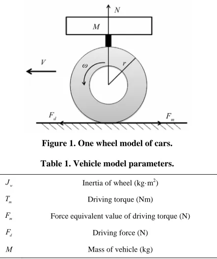
the longitudinal direction is described here. For simplic- ity, one wheel model directly driven by an electric motor is used for the derivation of control law and numerical simulations. Although the one wheel model is quite sim- ple, it still retains the essential dynamics of the system. In deriving the dynamic equations of the system, the lat- eral and vertical motions are neglected. The rolling re- sistance and air resistance are also ignored. A simple one wheel model is shown in Figure 1.

The dynamic equation for the w

d longitudinal vehicle motion are given by

J T rF (5)

d

MVF

m m

T rF

(6) (7)



where  is the angular velocit

l r

d

y of wheel, r the radius of whee and V the vehicle body speed. Othe parameters are defined in Table 1.

The tire driving force F is given by

 

, d

F  c (8) where

N





 

c,

  is the friction co and the

efficient as hereinafter defined normal tire force N is defined as

[image:3.595.63.284.85.349.2]

Figure 2. Relationship between slip ratio and friction co- efficient.

Figure 1. One wheel model of cars.

w

Table 1. Vehicle model parameters.

J Inertia of wheel (kg·m2₎

m

T

m

Driving torque (Nm)

F Force equiv torque (N)

d

alent value of driving

F Driving force (N)

M Mass of vehicle (kg)

here

w g is the acceleration of gravity.

The friction coefficient 

 

c, , which is the ratio between the driving force and the normal tire force, de- pends on the road condition (represented by road surface condition coefficient c) and the wheel slip (represented by slip ratio ). The slip ratio is defined as

w

V V

 

w

V (10)

ere Vw r

wh   is wheel speed. The slip ratio of 1

erizes th e slip

charact e wheel is completely skidding. If th ratio gets the value 0, no skidding is happening at the point of contact o with road.

The friction coefficient f tire

 

c,

  is a function of road surface condition coefficient c and slip ratio , which is called Magic-Formula and given in [14] by

 



35 0.35



, 1.1 e e .

c c  

  _{   }  _ 

(11)

Figure 2 shows the relationship between f fic

riction coef- ient  and slip ratio  on the road surface con- ditions r dry asphalt



c0.8



, wet asphalt

proximately  .

ion of Reference Slip Ratio λ* 3.2. Derivat

Let us choose the function  c

 

defined as

 



0.35



1.1 e e .

c

     35   (12) By using Equation (12), Equation (11)

as

can be rewritten

 

c, c _c

 

.

     (13) From Figure 2, evaluating the values of  which

 

c,

maximize   for different fin



0



c c means to d the value of  where the maximum val of the function

ue

 

c

  can be obtained. Let

 

d

0

d c  (14) and solving Equation (14) gives

log100 35 0.35

 

 (15)

0.13.

fo



c0.5



and ice road



c0.12



represents how - tion coefficien

. It also the fric t  increases with slip ratio  up to a value *





0.10.2 where it obtains e maxi- mum v e ficient. As defined in Equation (8), the driving force also reaches the maximum value corresponding to the friction coefficient. However, for satisfying

th coef

alu of friction

 _ 

, the friction coefficient decreases to the minimu e where the wheel is completely skid- ding. In consequence, to obtain the maximum value of

m valu

driving force, it is expected to control the slip ratio ap-

 Accordingly, for differe

0.13

(16) nt road conditions, when

  is met, the maxi ac

mum driving force can be hieved. In this paper, the value of reference slip ratio



is se

sli be kept at the reference value stably an

Electric Energy Consumption t to 0.13.

To obtain the maximum driving force all the time, the p ratio needs to

d accurately on any cases, but in fact the road surface on which vehicles travel is not at a constant condition always. Besides, the mass of vehicle varies when the weight of load such as the luggage and passengers changes. Consequently, we need to control the slip ratio under the condition of the often change of vehicle mass and road condition.

3.3. Evaluation of

[image:3.595.311.536.88.203.2]

we make the following assumptions. Assumption 1, the electric energy consumed by motor is all used to drive the wheel. Assumption 2, the energy consumed is equal to the work of motor. Then, the total electric energy consumed Ec can be written by the driving torque of

motor T tm

 

and the angle of rotation 

 

t as

   

0 d .

t

c m

E 

_

T     (17)

4. SMC with Integral Action fo

Control

C wi ction is proposed. Without loss of general-

r Slip Ratio

For slip ratio control, a nonlinear controller using SM th integral a

ity, the control law is derived based on the one wheel model mentioned above. The system dynamics can be written as

m

f bT

  ₍₁₈₎

where  R is the state of s ratio of driving wheel which is defi

ystem representing the slip ned as Equation (10) in situation of acceleration. T_m is the control input.

Differentiating Equation (10) with respect to time



1



_w

V  V

   w

V (19)

And substituting Equations (5), (6

tion (19), the following equations can be obtained,

 

) and (8) into Equa-





2

 

1 1 ,

g r M

f c

w w

V  J  

 

  _   _ (

  20)



1



. w w r b J V  

 (21)

objective

ratio to the constant re nce value

The control is to control the value of the slip fere .

of ggage. Besides, th

Actually, the mass of vehicle often changes with the number of passengers and the weight lu

e vehicle always travels on various kinds of road sur-faces. As a result, the controller needs to perform much robustly with the uncertainties affecting on the mass of vehicle and road surface condition which are represented by M and c respectively. The ranges of variation in

M and c are set as

min

M M M

 

max

n max

c c c (22) Equation (

tion f is not exactly known, but it can be estimated as ˆ

mi

Consider the system 18), the nonlinear func- f . The estimation error on f is assumed to be bounded by a known function FF

 

 ,

ˆ

f  f F. (23)

The uncertainty in f is due t Accordingly, by using Equation ca

o the parameter M and c. (20) the estimation of f n be defined as





 

ˆ

1 1 ,

w w

c

2 _ˆ

ˆ g r M

f

V  J  

 

     

  (24)

where Mˆ is the estimated value of M mated for c.

, w e

ely by using the arithmetic mean of the va

and ˆc is esti- Here e define the estimated values of thes parame- ters respectiv

lue of the bounds as

min max

ˆ M M

M  

min max

2

ˆ .

2

c c

c 

(25)

From these definitions, the error in estimation can be given by

ˆ f f





 











 



max 2 max max ˆ , , ˆ _ˆ

1 , , .

w

w

g _{c c}

V r

M c M c

J               (26)

Then, we let





 











 



max 2 max max ˆ , , ˆ _ˆ

1 , , .

w

c c

r

M c M c

J             (27)

4.1. Design of Sliding Surface

w

g F

V 



Letting  then the order of e sliding function of be the variable of interest,

system is assumed to be one. Th conventional SMC can be given by

 

,

c

s  t  ₍₂₈₎

where  is the error between the reference value, which is de

the actual slip ratio and fined as     . By adding an integral item to the sliding function

 

, c

s  t , the new sliding function s

 

,t can b - te

0

i

e writ n as

 

, t

 

d

s  t   K

_

   (29) where Ki is the integral gain, Ki0.

aw

oller is derived to

4.2. Derivation of Control L

In this section, the sliding mode contr

make the slip ratio  converge to the reference value

*

. The sliding mode happens when the trajectory

reaches the sliding surface defined by s0. The dy- namics of sliding mode is governed by

0.

s (30) Differentiating Equation (29), then sub ing the re- sult into Equation (30) gives

stitut



  



Ki



 



0 (31) The reference slip ratio λ* is

 

a constant, thus 0. Substituting Equation (18) into Equation



(32 input as

(31) gives





0.

m i

f bT K    ) and solving Equation (32) gives equivalent control





1

.

meq i

T f K

b  



 

 _   _ (33)

Then the estimate of the uivalent control input can be obtained as

eq





1 _ˆ

ˆ _.

meq i

T f K

b  



 

 _   _ (34)

For meeting the sliding condition (making the system trajectory in the sliding mode) despite

the dynamics f, the hitting control input is defined as uncertainties on

 

1

sgn

mht

T K s

b

 _ _ (35)

where 0 0 0 1 0       (36) and

 

sgn 1 s s s s    

K is called sliding gai u be given by

n. Th s, the control law can





 

ˆ

1 _ˆ

sgn .

i

m meq mht

T T T

f K K s

b   

When there is no existing in t dynamics (i.e., no variatio d M), Tmht

to be 0. Because Equation ontains the estimate of th

 

 



uncertainty n in c an

(37) c

 

  (37)

he system is desired e equivalent control Tˆmeq, Tm keeps the trajectory on

the sliding surface (s0, i.e.,   ). Because of the uncertainties, the trajectory deviates from the sliding surface. The hitting control act to return the trajectory back to the sliding surface whic ies the robustness of SMC.

Here, the sliding gain

s h impl K is chosen as

K F  (38) with the value of F given by Equation (27).  is a desig

strictly positive constant.

ap

n parameter described in Equation (4), which is a

Then choose a Ly unov functionas

2

(39) and differentiate Equation (39) with respect to time, that gives

1

V  s

2

2

1 d 2 d

V s ss

t

 

 _{ (40)}

Substituting Equations (18), (30), (34), (35) and (37) into Equation (40) yields

 





ˆ _sgn ˆ . V ss s f 

f K s

s f f K s

F s K s

s      _  _        (41)

Thus, the control law introduced in Equation (37) can guarantee the stability of the system in the Lyapunov sense under variations. Concretely, the stability of the sy

, the switched at an infinite frequency. rs have time delays and

 _

stem is guaranteed with an exponential convergence once the sliding surface is encountered, when the sliding condition is satisfied. So Equation (41) guarantees that the trajectory will converge to the sliding surface in finite time if the error is not zero. That is to say, slip ratio can be suppressed to the reference value in finite time when- ever the uncertainties occur in the system.

4.3. Chattering Reduction

In design of sliding mode control system control law requires switching

However, because the actuato

other imperfections, the action can lead to chatter in a neighborhood of the sliding surface. To reduce the chat- tering, the hitting control Tmht can be rewritten by using

the saturation function 1 mht s T K b sat     _ _{ }     

where 0

(42)

  is a design parameter re width of the boundary layer around

0 s

presenting the the sliding surface and the saturation function is defined as

 1 s s s sat s        1 s _                (43)

Thus, by using Equations (37), (38) a

trol law of the system by the proposed SMC can be re- written as









1 _ˆ

.

m i

s

T f K F sat

b   



  

 _     _{ }

  

  (44)

c s M 1200 (kg) and

5.1. Results of Robustness to the Variation in

In order to verify the robustness of proposed SMC with ion,

the v s made by assigning

5. Numerical Simulations

The numerical simulations have been done using MAT- e computer platform is

lations as follows. The first phase, the tim

LAB/Simulink software [15]. Th listed in Table 2.

The simulation conditions are described here. The simulation time is set to 10 (s) in all. There are three phases in the simu

e is from 0 (s) to 2 (s) and the car travels on the dry asphalt. The second phase, from 2 (s) to 8 (s), the car travels on ice road. The last phase, the car runs on wet asphalt during 8 (s) to 10 (s). The width of the boundary layer  defined in Equation (42) is set to 1. In Equa- tion (44), the proposed SMC law can be calculated with the values of design parameters Ki and , which both

impact on the steady state accuracy. Here, in order to confirm the effectiveness for the energy conservation performance of the proposed me d, the alues of both parameters are chosen as K_i 10

tho v

 and 1, which are determined by trial and error.

By using Equations (28), (30), (35) and (38), the con- trol law of the conventional SMC can be der ed as iv





1 _ˆ

.

mc

s

T f F sat

b 

  

 _   _{ }

  

  (45)

Likewise, in the conventional SMC, the parameters 1

 and  1. The values of paramet simulations are listed in Table 3.

produ

ed by the driver. Here, th

ers used in the As the input to the simulation of system, the torque is ced by the pressure on the accelerator pedal, which is decided on the car speed desir

e car speed is desired to achieve 180 (km/h) in 15 (s) by a fixed acceleration after starting the car. The range of variation in mass of the car M and road condition coeffi- cient c are imposed as Mmax 1400 (kg), Mmin1000

(kg), cmax 0.9 and cmin 0.1 respectively. So the

nominal values of mass and road condition coefficient

Tab mputer or the simulations.

[image:6.595.311.534.446.720.2]

OS Windows Vista (TM) Ultimate 32 bit le 2. Co platform f

CPU Intel (R) Core (TM) 2 Duo CPU T8100 2.10 GHz

RAM 4.0 GB

Hard Driver 250 GB 7200SATA RPM

ble 3. eters used in the simulations.

Jw 21.1 (kg·m2)

Ta Param

: Inertia of wheel

r: Radi

λ*_{: Reference slip ratio 0.13} )

us of wheel 0.26 (m)

g: Acceleration of gravity 9.81 (m/s2

an be obtained a cˆ0.5.

Mass and Road Condition

variation both in the mass of the car and road condit ariation in the mass of the car i

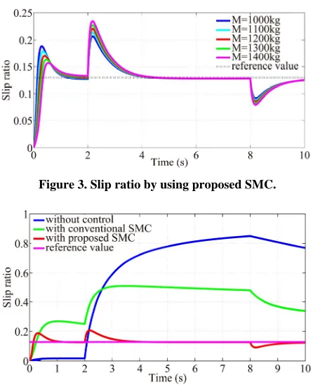
the value of M to 1000 (kg), 1100 (kg), 1200 (kg), 1300 (kg) and 1400 (kg) respectively. Figure 3 shows that the responses of slip ratio with different masses can con- verge to the reference value under the variation in the road condition. It is known that when the mass gets the nominal value 1200 (kg), in the first 2 (s), the response is more accurately than the car with other masses. But after 2 (s), the performance drops down with the mass in- creasing.

Next, we compare the proposed SMC with the con- ventional SMC and the case no control method used in the system.

Figures 4-8 show the responses of slip ratio under three different road conditions for five different masses respectively. The responses with proposed SMC can sup- press the slip ratio to the reference value 0.13 accurately in a very short time whenever both of the mass and road condition are changing. In addition, the slip ratio with the conventional SMC does not converge to the reference value because of the steady state error. When the car starts off at 0 (s) or runs into an ice road at 2 (s), the slip ratio response using control method grows with the in-

[image:6.595.54.284.593.651.2]

Figure 3. Slip ratio by using proposed SMC.

[image:6.595.58.284.679.737.2]

[image:7.595.71.275.85.200.2] [image:7.595.71.275.230.343.2] [image:7.595.74.273.373.483.2]

Figure 5. Slip ratio with mass of vehicle equals 1100 (kg).

[image:7.595.69.275.510.626.2]

Figure 6. Slip ratio with mass of vehicle equals 1200 (kg).

Figure 7. Slip ratio with mass of vehicle equals 1300 (kg).

Figure 8. Slip ratio with mass of vehicle equals 1400 (kg).

creasing wheel speed as a result of too much torque gen- erated. As the car travels from ice road to wet asphalt from 8 (s), the slip ratio decreases with the decreasing wheel speed, when the torque generated at that time cannot meet that required on the wet asphalt. The car without control is to make the slip ratio to 0, so at the first stage the response is converged to 0. However, when

the car runs into the ice road at 2 (s), the wheel spins out of control resulting that the wheel speed increasing sud- denly, which leads to a large slip ratio value. Therefore, we can see that the proposed SMC have a good perfor- mance against the variation in both of the mass of the car and road condition.

5.2. Results of Acceleration Performance

It is different from the simulation condition described in p

e ice road because the car cannot get road. revious that the simulations are executed under un-hanging road condition and mass every time. Figure 9

c

shows the time required for 100 meters by the car with different control method. The x-axis label indicates the cases of different road condition and mass, for example, DA1000 says that the car with the mass 1000 (kg) is driving on the dry asphalt, WA1200 shows that the case with the mass 1200 (kg) on the wet asphalt and IR1400 is the case with mass 1400 (kg) on the ice road. As shown in the bar graph, it takes the minimum time for the car with the proposed method for the 100 meters in every case. So we can see that the car with proposed SMC have gained the best acceleration. In other words, the results also indicate the car with the proposed SMC decreases the loss of driving force mostly. Moreover, the time re- quired is long on th

enough driving force to accelerate on the slippery 5.3. Results of Energy Conservation

To confirm the effectiveness of the proposed SMC for energy conservation, we compare it to the conventional SMC and no control method. As a numerical example, we calculate the energy consumed in the simulations executed in 5.1. Figure 10 shows the results of electric energy consumed by different mass cases.

[image:7.595.312.539.591.720.2]

We can see that the proposed SMC consumes the minimum energy in every case. The car without control takes most energy because the spin of wheel on the ice road from 2 (s) to 8 (s) leads to much energy loss. As the mass increases, the amount of energy cost decreases be- cause the car suppresses the spin of wheel by increment

[image:8.595.63.285.86.210.2]

Figure 10. Electric energy consumed by mass.

of mass to get more driving force. Conversely, the energy consumption with the proposed SMC and conventional SMC increases due to the rising cost of control as the mass increases. From this perspective, it also implies that an EV should be made more light to save more energy.

6. Conclu

This paper proposed an extended SMC method ad the integral term to the sliding function for improvin performance of the slip ratio control for EVs. The control objective focused on suppressing the slip ratio to the ref-erence value within the specified variation in ma vehicle and road conditions which allowed the vehicle to get the maximum driving force and minimum energy cost during acceleration.

As numerical examples based on the one wheel model, the simulations using the proposed method were ex

cuted, ed in

ass of vehicle and road conditions was verified. Be-

parameter

sions

ding g the

ss of

e- and the robustness to the uncertainties caus m

sides, by comparing to conventional SMC and no control, the vehicle with proposed method performed best accel- eration performance; moreover, the results also showed that the proposed method could reduce the energy cost when the vehicle travels on a slippery road.

In our research, the design  and the gain

i

K of integral item added in the sliding function was determined by trial and error, so it is necessary to de- velop a method to find the optimal value of  and gain

i

K . Moreover, although the effectiveness of the pro- posed method for traction was just verified in the accel- eration situation in this paper, we need to verify and im- prove the method for overall driving condition including braking situation. Then, the method is expected to be im- plemented and be one of the advanced motion control of EVs.

REFERENCES

[1] S. Brown, D. Pyke and P. Steenhof, “Electric Vehicles: The Role and Importance of Standards in an Emerging

3806. doi:10.1016/j.enpol.2010.02.059

[2] T. Hirota, M. Ueda and T. Futami, “Activities of Electric il

gineers, Vol. 50, No. 3, 2011, pp. 195- 200.

[5] Y. Hori, “Sim dhesion Control of

4WD Electric hnical Meeting on

tric Vehicle by Vehicles and Prospect for Future Mob ity,” Journal of the Society of Instrument and Control Engineers, Vol. 50, No. 3, 2011, pp. 165-170.

[3] T. Sakai and Y. Hori, “Advanced Vehicle Motion Control of Electric Vehicle Base on the Fast Motor Torque Re- sponse,” Proceedings of the 5th Annual International Symposium on Advanced Vehicle Control, Michigan, 2000, pp. 729-736.

[4] R. Shitato, T. Akiba, T. Fujita and S. Shimodaira, “A Study of Novel Traction Control Method for Electric Propulsion Vehicle,” Journal of the Society of Instrument and Control En

ulation of MFC-Based A Vehicle,” Papers of Tec

Industrial Instrumentation and Control, Vol. 2C-00, No. 1-23, 2000, pp. 291-293.

[6] T. Kawabe, Y. Kogure, K. Nakamura, K. Morikawa and T. Arikawa, “Traction Control of Elec

Model Predictive PID Controller,” Transaction of Japan Society of Mechanical Engineers, Series C, Vol. 77, No. 781, 2011, pp. 3375-3385. doi:10.1299/kikaic.77.3375

[7] C. Unsal and P. Kachroo, “Sliding Mode Measurement Feedback Control for Antilock Braking Systems,” IEEE Transaction on Control Systems Technology, Vol. 7, No. 2, 1999, pp. 271-281. doi:10.1109/87.748153

[8] M. Oudghiri, M. Chadli and A. E. Hajjaji, “Robust Fuzzy Sliding Mode Control for Antilock Braking Systems,”

oup, Boca Raton, 2009.

EE Transaction on Industrial International Journal on Sciences and Techniques of Automatic Control, Vol. 1, No. 1, 2007, pp. 13-28. [9] V. Utkin, J. Guldner and J. Shi, “Sliding Mode Control in

Electro-Mechanical System,” 2nd Edition, Taylor & Fran- cis Gr

[10] K. Nonami and H. Tian, “Sliding Mode Control,” CO- RONA, Tokyo, 2000.

[11] J. Y. Hung, W. Gao and J. C. Hung, “Variable structure Control: A Survey,” IE

Electronics, Vol. 40, No. 1, 1993, pp. 2-22.

[12] J. J. E. Slotine and W. Li, “Applied Nonlinear Control,” Prentice-Hall, Inc., New Jersey, 1991.

[13] I. Eker and A. AKinal, “Sliding Mode Control with Inte- gral Augmented Sliding Surface: Design and Experimen- tal Application to an Electromechanical System,” Elec- trical Engineering, Vol. 90, No. 3, 2008, pp. 189-197. doi:10.1007/s00202-007-0073-3

[14] H. B. Pecejka and E. Bakker, “The Magic Formula Tyre Model,” Proceedings of the 1st International Colloquium on Tyre Models for Vehicle Dynamics Analysis, Vol. 21, Suppl. 001, 1991, pp. 1-18.