www.hydrol-earth-syst-sci.net/17/295/2013/ doi:10.5194/hess-17-295-2013
© Author(s) 2013. CC Attribution 3.0 License.
Earth System
Sciences
Conceptual and numerical modeling approach of the
Guarani Aquifer System
L. Rodr´ıguez1, L. Vives2, and A. Gomez1,3
1Centro de Estudios Hidroambientales, Facultad de Ingenier´ıa y Ciencias H´ıdricas, Universidad Nacional del Litoral, CC 217, 3000, Santa Fe, Argentina
2Instituto de Hidrolog´ıa de Llanuras, Universidad Nacional del Centro de la Provincia de Buenos Aires and Comisi´on de Investigaciones Cient´ıficas de la Prov. de Buenos Aires, Italia 780, B7300, Azul, Argentina
3CONICET, Consejo Nacional de Investigaciones Cient´ıficas y T´ecnicas, Argentina
Correspondence to: L. Rodr´ıguez ([email protected])
Received: 14 August 2012 – Published in Hydrol. Earth Syst. Sci. Discuss.: 30 August 2012 Revised: 15 November 2012 – Accepted: 17 December 2012 – Published: 25 January 2013
Abstract. In large aquifers, relevant for their considerable size, regional groundwater modeling remains challenging given geologic complexity and data scarcity in space and time. Yet, it may be conjectured that regional scale ground-water flow models can help in understanding the flow system functioning and the relative magnitude of water budget com-ponents, which are important for aquifer management. The Guaran´ı Aquifer System is the largest transboundary aquifer in South America. It contains an enormous volume of water; however, it is not well known, being difficult to assess the impact of exploitation currently used to supply over 25 mil-lion inhabitants. This is a sensitive issue because the aquifer is shared by four countries. Moreover, an integrated ground-water model, and therefore a global ground-water balance, were not available. In this work, a transient regional scale model for the entire aquifer based upon five simplified, equally plau-sible conceptual models represented by different hydraulic conductivity parametrizations is used to analyze the flow sys-tem and water balance components. Combining an increas-ing number of hydraulic conductivity zones and an appro-priate set of boundary conditions, the hypothesis of a con-tinuous sedimentary unit yielded errors within the calibra-tion target in a regional sense. The magnitude of the water budget terms resulted very similar for all parametrizations. Recharge and stream/aquifer fluxes were the dominant com-ponents representing, on average, 84.2 % of total inflows and 61.4 % of total outflows, respectively. However, leakage was small compared to stream discharges of main rivers. For in-stance, the simulated average leakage for the Uruguay River
was 8 m3s−1 while the observed absolute minimum dis-charge was 382 m3s−1. Streams located in heavily pumped regions switched from a gaining condition in early years to a losing condition over time. Water is discharged through the aquifer boundaries, except at the eastern boundary. On av-erage, pumping represented 16.2 % of inflows while aquifer storage experienced a small overall increment. The model water balance indicates that the current rate of groundwa-ter withdrawals does not exceed the rate of recharge in a regional sense.
1 Introduction
The Guaran´ı Aquifer System, hereafter GAS (also known as SAG from its Spanish and Portuguese name), is the largest transboundary aquifer system in South America. It extends for some 1.2 million km2over four countries: 70 % in Brazil, 19 % in Argentina, 6% in Paraguay, and 5 % in Uruguay (Fig. 1). The aquifer is formed by sandstones and confined by basalts in about 90 % of its extent. Sandstones outcrop along aquifer edges, deepening toward the center of the basin, where they can reach a maximum thickness of some 600 m and depths of 2200 m.
Fig. 1. Location of the Guaran´ı Aquifer System. Boundaries of GAS
groundwater flow models: (1) this work; (2) Vives et al. (2001); (3) Vassolo (2007); (4) SNC Lavalin Internacional (2008a); (5) SNC Lavalin Internacional (2008b); (6) SNC Lavalin Interna-cional (2008c); (7) SNC Lavalin InternaInterna-cional (2008d); (8) G´omez et al. (2010); (9) Heine (2008); (10) Rabelo and Wendland (2009).
countries. These peculiarities are not specific to GAS. Other large aquifers relevant for their considerable size are the High Plains Aquifer in the USA (Luckey and Becker, 1999), the Nubean Aquifer shared by Egypt, Chad, Sudan and Lybia (Robinson et al., 2007), the Great Artesian Aquifer in Aus-tralia (Habermehl and Lau, 1997), the Yrenda-Toba-Tarije˜no Aquifer System shared by Argentina, Bolivia and Paraguay (UNESCO-IHP, 2009), and the Navajo Aquifer System in the USA (Heilweil et al., 2002).
To address these issues and aim towards sustainable man-agement and development of the GAS, the Global Enriron-mental Facility (GEF) financially supported the four coun-tries to develop the “Proyecto para la Protecci´on Ambien-tal y Desarrollo Sostenible del Sistema Acu´ıfero Guaran´ı – PSAG” (Environmental Protection and Sustainable Devel-opment Project for the GAS). The PSAG was a multidisci-plinary scientific effort and regional collaboration requiring good cooperation between various disciplines. The project revealed some of the difficulties associated to the study of regional aquifers.
In this article, like in the recent work of Barthel (2011), the term “regional scale” refers to areas of approximately 105–106km2 in size. Some of the largest aquifers in the world have been studied for diverse purposes and with dif-ferent modeling approaches. For instance, the US Geologi-cal Survey and the Oklahoma Water Resources Board, USA, conjunctively developed a groundwater flow model of the High Plains Aquifer to be used for allocating the amount of water withdrawn from the aquifer (Luckey and Becker, 1999). The Nubean Sandstone Aquifer has been studied for many years. A preliminary modeling effort on this aquifer was reported by Heinl and Brinkmann (1984), who used a finite element model to address various basic questions re-garding the dynamics of the aquifer. In a recent work, Gos-sel et al. (2004) presented an integrated GIS-based ground-water flow model for the Nubean Aquifer intended for im-proving previous modeling efforts. A transient groundwa-ter model was constructed for the Great Artesian Basin for management purposes (Welsh, 2006). One recent contribu-tion to regional-scale groundwater modeling was given by Michael and Voss (2009), who focused their work on the es-timation of regional-scale aquifer properties in the Bengal Basin of India and Bangladesh. In order to accomplish their objective, they combined inverse groundwater modeling us-ing measured heads, model calibration usus-ing estimated water ages, and statistical analysis of driller logs.
Several local-scale groundwater models were built in the GAS, either to meet local or state requirements or to ana-lyze a particular behavior/characteristic of the aquifer. Here, the term “local scale” refers to models covering areas of approximately 103km2. A thorough study of the aquifer within Paraguayan territory culminated with a multi-layer, steady state groundwater flow model (Vassolo, 2007). Within Brazilian territory, Heine (2008) built a MODFLOW model to quantify recharge for management purposes around the city of Ivoti in southern Brazil, while Rabelo and Wend-land (2009) assessed groundwater recharge and water fluxes in the state of Sao Paulo, Brazil, through a numerical, fi-nite element model, covering over 5000 km2of outcropping sandstones. Within the PSAG project, four pilot areas were selected for detailed study on the basis of their distinct hy-drogeologic conditions and potential groundwater exploita-tion conflicts. In each of them, a local-scale flow model run under MODFLOW intended for management practices was developed (SNC Lavalin, 2008a, b, c, d). Recently, G´omez et al. (2010) implemented MODFLOW (Harbaugh et al., 2000) on a region located along the Brazilian–Uruguayan border in order to validate a newly proposed multi-layer conceptual model, verify previous recharge estimates and test future ex-ploitation scenarios. The location of these and all other mod-eling sites/boundaries described in this section are indicated in Fig. 1.
built upon scarce geologic and hydrogeologic data. It was a finite element, two-dimensional, steady state model, which extended over 60 % of the currently identified aquifer area. Regional geologic structures that may condition groundwa-ter flow were included in the model, and a handful of short stream reaches in outcropping areas to the east were explic-itly simulated. Nonetheless, many questions remained unan-swered or partially addressed due to the simplifications set forth during the modeling process, for example: Where is the south-western boundary of the aquifer located? What are the most likely discharge zones in the southern sector? Could reaches along the Paran´a and Uruguay rivers be po-tential discharge zones? What is the dynamics of the sys-tem along the aquifer western boundary? How important are stream/aquifer interaction processes in outcropping ar-eas compared to other mass balance components? Are there local recharge/discharge systems identified within a regional context? More importantly, the overall water balance of the aquifer is not known.
Field data generated during the PSAG allowed revisiting the conceptual model, proposing a new southern boundary for the aquifer and postulating its interaction between nu-merous streams (Gastmans et al., 2012). The newly pro-posed conceptual model was numerically validated by Vives et al. (2008), who also hypothesized and numerically tested that the GAS may discharge through selected reaches along the Uruguay and Paran´a rivers. Yet, the magnitude of these discharges is unknown.
All groundwater flow models built so far on the GAS, ei-ther at local or regional scale, were run under a steady state regime, which, in turn, limits their use as learning tools as well as management tools. In this work, a transient regional scale model covering the full extent of the GAS is presented. The new model complements its steady state predecessor by Vives et al. (2008), rendering the new modeling approach more informative in the process of enhancing the current hy-drogeologic understanding of the aquifer and its potential use as a management device of subsurface resources.
The model was used to test whether the aforementioned questions can be modeled consistently with aquifer head data. It was also instrumental for evaluating water balance components for the entire aquifer, emphasizing the role of processes such as the stream/aquifer interaction as a lead-ing discharge mechanism in outcropplead-ing areas, and the feasibility of some aquifer discharge in the southern por-tion of the aquifer, a hypothesis that was disregarded in previous studies.
2 Location, geology and hydrogeology
Only a brief description of the main physiographic, geo-logic and hydrogeogeo-logic characteristics of the aquifer is pre-sented here. Further details about the GAS are given by Bi-garella and Salamuni (1961), Gilboa et al. (1976), Z´alan et
al. (1990), Ara´ujo et al. (1999), Campos (1998, 2000), and Rosello et al. (2006), among others. All technical reports resulting from the PSAG can be found at http://pag-ar00. minplan.gov.ar/SAG/.
The GAS is located between 16° S and 32° S latitude and 47° W and 56° W longitude underlying the R´ıo de La Plata drainage basin in South America (Fig. 1). Ground elevations vary from 1700 m a.s.l. (meters above sea level) in the south-eastern border down to approximately 30 m a.s.l. within Ar-gentinean territory. Due to its considerable extent and varia-tions of relief, diverse climates are identified. Mean annual, altitude-dependent precipitation shows a southward gradient, from 2000 mm in the north to 1400 mm in the south while mean temperature is above 20◦C almost everywhere. Mean annual evaporation has been estimated to be around 60 to 70 % of the annual precipitation.
The GAS sedimentary sequence consists of aeolian, and fluvial weakly-cemented sandstones beds of Upper Jurassic-Lower Cretaceous age deposited in parts of the tectonic Paran´a Basin and Chaco-Paran´a Basin (Ara´ujo et al., 1999). Sandstones range in thickness from a few meters in outcrop-ping areas along western and eastern aquifer boundaries, to more than 600 m at the center of the basin. Upper Cretaceous basalt flows as thick as 1500 m and varying degrees of frac-turing/fissuring cover 90 % of sandstone deposits. The strati-graphic sequence completes with Quaternary, non-uniformly distributed sediments. Figure 2 shows a simplified geologic map and transverse and longitudinal geologic profiles (Fos-ter et al., 2009). There has been intense debate as to whether the aquifer can be regarded as a single, continuous unit or is it actually separated in geologic compartments that may or may not introduce regional flow discontinuities (Ferreira, 1982; Campos, 1998; Soares, 2008). At regional scale, the GAS can be conceptualized as a sedimentary formation, spa-tially continuous, composed of sandstones, confined by un-derlying pre-GAS deposits, and overlying post-GAS deposits (see Fig. 2), except in outcropping areas.The GAS is assumed to range from unconfined to semi-confined in recharge areas. Towards the center of the tectonic basins, it becomes increas-ingly confined due to the thickening of overlying basalts, which leads to artesian conditions over large areas.
Fig. 2. Simplified geology showing pre-GAS and post-GAS sediments, GAS outcropping areas and potentiometric lines; (A), (B), and (C): longitudinal and transverse geologic profiles (reproduced with permission from Foster et al., 2009).
a “continuous groundwater body” across the entire region”. Regional flow is from northeast to southwest. In outcrop-ping areas, predominantly-recharge regions alternate with predominantly-discharge ones. The latter may discharge re-gional as well as local flows.
Recharge to the GAS occurs by infiltration of excess rain-fall in outcropping regions, which cover approximately 10 % of the entire aquifer extent. Estimates of recharge rates range from 10 % (Reboucas, 1976) to 4 % (Chang, 2001) of mean annual precipitation. So far, there is no evidence of recharge from streams. However, it should not be ruled out. Well with-drawals are considered the main source of discharge from the aquifer. Other sinks, though not well known, include seepage to streams and seepage to underlying/overlying formations.
Average salinity in recharge areas is about 50 mg L−1, and can be as much as 500 mg L−1on the southwestern region. With increasing depth and confinement, and following the general flow direction, the groundwater temperature also in-creases from 25 to 65◦C, an increment that has been mostly attributed to the effect of the normal geothermal gradient. A temperature effect on the aquifer’s hydraulic conductiv-ity (permeabilconductiv-ity) may be expected as a result of changing
kinematic viscosity. The isotherm map of the GAS devel-oped by Gastmans et al. (2012) is very informative, showing the highest values located within Brazilian territory; nonethe-less, about 65 % of the aquifer has temperatures between 25– 45◦C.
3 Conceptual hydrogeologic model
A new hydrogeologic conceptual model and a numerical model for the entire aquifer were end products of the mul-tidisciplinary work within the PSAG. Gastmans et al. (2012) put together a revised, much-improved conceptual model that incorporates many aspects that were overlooked in previous versions. As mentioned previously, from a regional point of view, the GAS was defined as a spatially continuous sed-imentary formation, composed of sandstones, confined by underlying pre-GAS deposits, and overlying post-GAS, i.e. basalts and quaternary deposits (see Fig. 2), except in out-cropping areas.
registered at the time of wells drilling. Therefore, they span a 30–40 yr time window starting in the 1970s and may not be representative of current conditions, especially in areas of in-tense pumping. Regionally, groundwater flows from recharge to discharge areas, presenting a directional trend from the northeast and northwest toward the center of the sedimentary basin and then south. This regional flow pattern is influenced by the tectonics of the geologic basins and its evolution, as pointed out by Ara´ujo et al. (1999). The potentiometric map reflects the presence of mega-structures. Hydraulic gradients are steeper at or near outcropping areas, with values as high as 3 to 5 m km−1 in the northeast, 2 to 3 m km−1 at east-central locations and 1.5 to 2 m km−1at the west-northwest. They decrease toward the center of the sedimentary basin as the aquifer deepens. In spite of the presence of structural dis-continuities at different spatial scales, groundwater flow con-tinuity still persists at regional scale (Gastmans et al., 2012; Foster et al., 2009).
Hydraulic connection across confining layers has been poorly addressed, though it is likely. At present, available data are limited for assessing and quantifying inter-layer ver-tical occurrence, its direction and its magnitude. Based on a handful of deep wells that tap underlying Permian deposits, Gastmans et al. (2012) postulated that the GAS lies over an erosive basal surface extended over parts of the Paran´a sedi-mentary basin, putting the GAS in contact with argillaceous, low permeability units in the north; silty-clayed, more per-meable formations at the center and silty-sandy formations of moderate permeability in the south. Neuzil (1994) reported argillaceous permeability for both lab test and regional scale studies, relating porosity from different materials to per-meability to identify possible trends. For clayed sandstone, this author suggested a hydraulic conductivity range between 8.6×10⁻⁵and 8.6×10⁻¹¹m d−1for flow parallel and normal to bedding, respectively, which are very low for a quantifiable GAS/pre-GAS hydraulic connection. Considering that inter-layer flow may be controlled by the less permeable material, the magnitude of vertical flows between sandstones and pre-GAS sediments may be assumed negligible.
Water quality data may help to elucidate the interlayer flow connectivity issue. This type of data is scarce and some of dubious quality to extract definite conclusions about the ex-istence of vertical density gradients; however, that possibility is feasible given the great extension of the aquifer. Manzano and Guimaraens (2009) exhaustively analyzed background hydrochemical information and field data generated during the PSAG, concluding that the aerial distribution of solutes such as TDS, Na, Cl and SO4, among others, is dominated by a mixture of GAS waters with saline waters from pre-GAS units. These authors also identified two mixture-dominated areas, suggesting the existence of vertical, upward flows from pre-GAS formations controlled by stratigraphic and struc-tural conditions. Nonetheless, they concluded that to date, the magnitude of those fluxes is completely unknown,
per-ceived to be rather small compared to other components of the regional water balance.
A number of authors sought evidence of the hydraulic connection between confining basalts and underlying sand-stones, showing divergent conclusive results. Reboucas and Fraga (1988) argued that water flow can predominantly oc-cur along horizontal discontinuities surfaces at the top and bottom of lava flows, i.e. at interflow contacts, and at ver-tical column disjunctions present at the center of flows. Given this type of flow description, restricted to specific ar-eas within the basalt packet, uncertainties regarding hydro-geologic units interconnections are still great (Lastoria et al., 2007). Most gathered evidence regarding GAS/basalts hydraulic connection belongs to the Sao Paulo and Mato Groso do Sul States in Brazil, located to the NE and NW of the aquifer, respectively. Fernandes et al. (2008) intensively studied basalts within Sao Paulo State, proposing a concep-tual model for water circulation within basalts around the Ribeir˜ao Preto area. In a recent work, Fernandes et al. (2012) used hydrochemistry and basalt fractures mapping to inves-tigate whether vertical conductive structures might conduct water. So far, they have found vertical fractures present only on dense layers that do not penetrate into vesicular layers pre-venting a hydraulic connection with sandstones underneath. Even though Lastoria et al. (2007) provided some evidence of ascending/descending flows within Mato Groso do Sul us-ing hydrochemistry, it would be speculative to extrapolate this condition to the entire aquifer. Hence, the current ver-sion of the conceptual model assumes neither recharge from nor discharge to confining basalts.
These conceptual simplifications regarding the layer struc-ture of the GAS imply an essentially two-dimensional flow regime at regional scale. Therefore, the model will be treated as two-dimensional.
One of the great uncertainties of the conceptual model is the location of regional discharge zones and the magnitude of discharge fluxes. Even though local recharge/discharge systems have been clearly identified in outcropping areas along the western and southern boundaries (see Fig. 2), re-gional discharge may occur through selected portions of the boundary or other sinks. In this work it is assumed that short reaches of the Paran´a and Uruguay rivers could discharge GAS water.
Net recharge, i.e. effective rainfall minus evapotranspira-tion, occurs along outcropping areas along portions of the aquifer boundary. If not intercepted by pumping or streams, some of it may become deep recharge.
4 Methods
based on the maximum likelihood method for parameter es-timation, as explained in Carrera and Neuman (1986). In essence, the values of hydraulic properties variable in space (and sometimes in time), are calculated based on a previous estimate of the parameters and measured values of heads (and concentrations if transport is solved).
It should be pointed out that, besides data errors and con-ceptual model uncertainties, there are also errors associated with the numerical method. The numerical error is related to the discretization, the numerical procedure and round-off errors. TRANSIN is flexible as to choose a weighting param-eter for flow 0≤θf ≤1; ifθf =0 it is an explicit scheme; if
θf =1 it is implicit; and ifθf =1/2 it is the Crank–Nicolson scheme of second order in time. More details on the theo-retical background of this model can be found in Medina et al. (1996).
5 Model structure
Following the definition by Carrera et al. (2005), parametrization is one element of model structure. In this work, different parametrizations for hydraulic con-ductivity are explored to improve model calibration. Five hydraulic conductivity zonations are proposed and evaluated through transient modeling along a 39-yr period based upon an annual time step, the first step being the steady state. 5.1 Finite element mesh
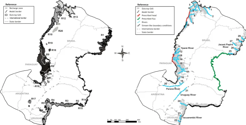
The model boundary extends to the entire GAS, as shown in Fig. 1. The two-dimensional domain was discretized into 46 862 triangular elements and 23 890 nodes using the mesh generator 2DUMG (Bugeda, 1990). Mesh refinements were introduced in areas of expected steep hydraulic gradients generally associated with heavy pumping in outcropping ar-eas, and in areas of steep topographic gradients in moun-tain regions located in the central/southeastern portions of the aquifer boundary. Elements area averaged 25 km2; the largest elements were located in the central region of the domain. The element size used here is similar to the cell size used in models of aquifers of comparable size, for example the Great Artesian Basin in Australia, where a uniform 5 km×5 km cell size was used (Welsh, 2006).
5.2 Spatial zonation of hydraulic conductivity
At the time of the construction of the conceptual and numer-ical models, there were not enough point hydraulic conduc-tivity (K) data as to construct a regionalized distribution map forKusing a tool such as kriging. An alternative approach to produce K maps was used instead.
Zonation is one of the methods to parametrize hydraulic properties needed to solve mathematical equations set forth in inverse modeling (Carrera et al., 2005), each producing an alternative model. Figure 3 shows five hydraulic
conductiv-ity zonings defined upon different criteria: (Z1) one zone, i.e. uniformK; (Z2) nine zones, their geometry closely replicat-ing the zonreplicat-ing previously defined by Vives et al. (2001) who defined hydraulic conductivity zones based on the location of main geologic structures; (Z3) seventeen zones, their geom-etry and boundaries delineated following changes on aquifer thickness; (Z4) nineteen zones, their geometry combining the patterns of the piezometric map, namely transitions of hydraulic gradients (see Fig. 2) and the zoning defined by Vives et al. (2001); and (Z5) thirty one zones, their geometry accompanying hydraulic gradients of the piezometric map more closely than Z4.
Limited and scattered information on hydraulic conduc-tivity from aquifer tests and anecdotal values served as pre-vious estimates. Freeze and Cherry (1979) indicated a max-imum threshold value for sandstones of 1–2 m d−1. Ara´ujo et al. (1999) and Sracek and Hirata (2002) reported values of 8.7 m d−1and 13 m d−1, respectively, for meanK in the Brazilian states of Sao Paulo, Paran´a and Rio Grande do Sul (see Fig. 1). Within Paraguayan territory, values of 1.6– 3.8 m d−1were reported by Vassolo (2007), whilst hydraulic conductivities between 0.12 and 5.76 m d−1, with an average of 1.5 m d−1, were published for northern Uruguay (G´omez et al., 2010).
The effect of temperature over the flow field was taken into account by correcting the hydraulic conductivity by means of the Schneebeli formulae (Custodio and Llamas, 1976)
k(θ )≈k(20◦C)θ+20
40 , (1)
withθ the temperature in◦C. Each finite element within a
given zone was assigned a K-value corrected for temperature. The temperature was interpolated from the isotherms map provided by Gastmans et al. (2012). Hydraulic conductivity was then converted to transmissivity in TRANSIN by multi-plying the corrected initial guess forKfor a given element by the mean thickness of the aquifer for that element. Initial K-values were recalculated through automatic calibration. 5.3 Boundary conditions, recharge, streams
and pumping
Fig. 3. Alternative conceptual models represented by zonings of hydraulic conductivity.
Fig. 4. Simulated boundary conditions, recharge areas and stream reaches (note: only the simulated reach of minor streams and major rivers
like the Paran´a and Uruguay rivers, are indicated; the full drainage network is omitted for the sake of clarity).
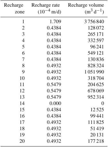
annual precipitation which varied from north to south ac-cording to the precipitation gradient previously mentioned; 3 % was imposed along the western area and 1.5 % along eastern and southern areas. Table 1 shows recharge rates and
[image:7.595.99.494.405.606.2]Table 1. Recharge rates and volumes over each simulated recharge
area.
Recharge Recharge rate Recharge volume
zone (10−4m/d) (m3d−1)
1 1.709 3 756 840
2 0.4384 128 072
3 0.4384 265 171
4 0.4384 332 597
5 0.4384 96 241
6 0.4384 549 121
7 0.4384 130 836
8 0.4932 828 324
9 0.4932 1 051 990
10 0.4932 318 704
11 0.5479 204 625
12 0.5479 678 069
13 0.5479 952 314
14 0.000 0
15 0.4384 12 525
16 0.4384 99 441
17 0.4932 111 825
18 0.4932 51 419
19 0.4932 20 131
20 0.4932 177 218
The value of that function represents anomalies with respect to the mean annual precipitation, i.e. a value of the time function equal to 1.2 for a particular year means that the an-nual precipitation for that year is 20 % higher than the mean annual precipitation. The precipitation series corresponding to the Rivera-Santana station located on the border between Uruguay and Brazil was used to construct Fig. 5, which was deemed indicative of the precipitation temporal variability. The value of the temporal function corresponding to the first time step is equal to one. The GAS underlies the R´ıo de la Plata Basin, the second largest in South America, charac-terized by a highly dense drainage network that discharges into the main waterways of the region: Paran´a, Paraguay and Uruguay rivers. In the occidental border, numerous streams drain toward the Paraguay River, located outside the model area, while the rest of the streams drain toward the Uruguay and Paran´a rivers. Stream–aquifer interactions were simu-lated along 29 streams reaches (see Fig. 4). For their quick location and analysis, all simulated rivers were identified by a number.
As previously described, there are still great uncertain-ties regarding discharge pathways, without which a sound water balance would be difficult to close. In this work, it was assumed that reaches along the Paran´a and Uruguay rivers, located in confined areas but nearby the region where the aquifer is closest to the surface, could interact with GAS waters.
Within TRANSIN, leakage between surface water bodies and the adjacent aquifer is computed as Q=α(h−Hext),
0,00 0,20 0,40 0,60 0,80 1,00 1,20 1,40 1,60 1,80 2,00
1 3 5 7 9 11 13 15 17 19 21 23 25 27 29 31 33 35 37 39
Ti
m
e
f
u
n
ct
ion
Year
REC
[image:8.595.73.261.91.347.2]PUM
Fig. 5. Time function for recharge and pumping applied to the
tran-sient simulation.
whereQis the stream leakage (L3T−1);αis the leakance co-efficient (L2T−1);his the piezometric head (L), andHext(L) is a reference, external water level. If field data is available Hextis usually the stream stage. In absence of such informa-tion, in this work, Hextwas interpolated from ground eleva-tions and piezometric levels, in the latter case only for the Paran´a and Uruguay river reaches. The leakance coefficient is the ratio between the stream cross sectional area times the hydraulic conductivity of streambed sediments, Kb, and the thickness of these sediments. The coefficient was estimated assuming Kb-values two orders of magnitude smaller than K-values for sandstones (around 1 m d−1 according to Freeze and Cherry (1979)), a thickness of streambed sediments equal to 1 m, and a cross-sectional area ranging from 100 to 1000 m2for all streams, except for the Uruguay and Paran´a rivers, for which higher values were adopted. Leakance co-efficients for the Paran´a and Uruguay rivers were 50 and 20 m2d−1, respectively, whilst for the rest of the streams were between 1 and 10 m2d−1. Sensitivity runs performed during the early stages of the model development showed no significant changes in model results for the range ofαtested. 5.4 Pumping
5.5 Calibration
The model calibration approach consisted of using a combi-nation of automated and manual methods. The primary ob-jective of the calibration was to minimize the difference be-tween simulated and observed hydraulic heads, while seek-ing hydrogeologic parameters values consistent with the cur-rent knowledge of the aquifer. Five diffecur-rent hydraulic con-ductivity zonations, i.e. models, were set forth using the cri-teria explained in Sect. 5.2, increasing the number of zones on each zonation pursuing the principle of parsimony whilst relating the zones geometry to different aquifer characteris-tics. Previous estimates of hydraulic conductivity for each zone were modified through automatic calibration.
Insufficient head data precluded performing a conven-tional modeling approach, i.e. model calibration for steady state with field data representing pre-development conditions as close as possible, and then use of the steady sate simulated aquifer head as the initial condition for the transient simula-tion. A different calibration strategy was used instead.
A 39-yr transient simulation with yearly periods, the steady state being the first time year of the time series, was performed. The model was calibrated against 317 observed piezometric levels. Those levels span a 30–40 yr time win-dow starting in the 1970s, therefore some may not be rep-resentative of current conditions in areas of intense pump-ing. Moreover, the reliability of some field data is question-able as wells may not be cased along confining units, re-sulting in an integrated reading that may be interfered by local-type flows. An additional source of error is the value of well elevation, which is needed for estimating piezomet-ric level, especially in areas of steep slopes. Observations are not evenly distributed across the study area; the majority of measurements are located near or at outcropping areas of the aquifer. Along the central region, where the aquifer reaches its maximum depth, data points are sparse. The absence of data is notorious within Argentinean territory. Observed lev-els range between a maximum of 1202 m a.s.l. and a min-imum of 10 m a.s.l. Head measurements were taken at the time of well drilling; about 70–80 % of the wells were con-structed during the last decade when there was a significant increment in groundwater exploitation not evenly distributed across the entire aquifer area. The rest of the measurements are spread in time since the seventies. Therefore, in the ab-sence of transient head data for calibration, all available ob-servations were assigned to the last period. Given the qual-ity of observations and the piezometric levels maximum– minimum range, the calibration target was set at±40 m for mean error statistics.
6 Results and discussion
Model performance and results were analyzed following var-ious criteria applied to piezometric levels, mass balance
com-Table 2. Goodness of fit estimators.
Kzones RMSE R2
Z1 1 58.27 0.922
Z2 9 53.12 0.934
Z3 17 45.81 0.950
Z4 19 42.13 0.958
Z5 31 36.99 0.968
ponents, hydraulic conductivity zonations and ranges of hy-draulic conductivity.
6.1 Piezometric levels
The optimized transient models were evaluated with respect to the match between observed and simulated piezometric levels. The root mean square residuals (RMS) were calcu-lated as follows (Zheng and Bennett, 1995):
RMS=
" 1
N
N X
i=1
(hobsi−hsimi)
2 #1/2
, (2)
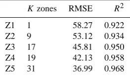
wherehsim andhobs are simulated and observed hydraulic head, respectively, andNis the number of observations. The subscriptiindicates observation number, while the term in parentheses is called model error. RMS values show an im-provement of model calibration as the number ofK zones increases (Table 2). It remained outside the calibration target for all but the last zonation reaching a minimum of 36.99 m.
The linear correlation coefficientR2varied from 0.922 for Z1 zonation to 0.968 for Z5 zonation, indicating a significant linear correlation between calculated and observed levels for all cases (Table 2). Figure 7 shows calibration results for sce-nario Z5. Model results closely replicate groundwater flow patterns concerning both flow directions and hydraulic gradi-ents. Regional groundwater flow is from northeast and north-west toward the center of the sedimentary basin and then south. Modeling results along the western boundary show that regional flow is disrupted by local recharge/discharge systems, a pattern present in the observed piezometric map of Fig. 2. The eastern boundary and adjacent areas are char-acterized by steeper simulated hydraulic gradients, in coinci-dence with observed gradients within highly exploited areas in the northeast and steep terrain in the central-east, while smoother gradients are encountered at the center of the sim-ulated area.
[image:9.595.362.494.81.159.2]Fig. 6. Simulated pumping wells and pumping zones with their corresponding groundwater extraction rates.
0 250 500 750 1000 1250
0 250 500 750 1000 1250
Observed (m)
Calculated
(m
)
Fig. 7. Simulated and observed piezometric levels (m a.m.s.l.) for
zonation Z5 (linear regression and contour map).
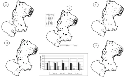
identifiable overestimated/underestimated regions. As shown in the histogram at the bottom of Fig. 8, the number of out-liers, i.e. points for which the absolute value of model error is greater than 80 m, reduces progressively as the number of
K zones increases. By the same token, the number of data points within the calibration target also increases reflecting
the improvement of model performance, though some ex-treme errors persist no matter whatK zoning is used. This can be explained by several factors. Firstly, alternative con-ceptual models based solely in theK parameter may be an acceptable approach at regional scale but it may be question-able at different spatial scales as the presence of geologic structures not explicitly included in the regional model may influence groundwater circulation. Secondly, calibration data are far from ideal, affecting in turn, model fit. Ideally, avail-ability of transient piezometric levels would be desirable. Only a single set of calibration data points was available with no identification of the time of measurement, limiting transient calibration strategies. This situation is particularly critical in areas of intense pumping. Then, observations were assigned to the last simulated year. Since pumping is very low in regional terms, this approach was considered reason-able, although it is recognized that it introduces calibration errors at local-meso spatial scales.
6.2 Water budget
An independent water balance for the entire aquifer is not available; nonetheless, qualitative and quantitative analyses are carried out wherever possible to verify the model water budget. Even though only results for scenario Z5 are shown in Fig. 9, water budget components were very similar for all zonations.
[image:10.595.51.281.380.583.2]
1
3
2 4
[image:11.595.83.510.66.330.2]5
Fig. 8. Residual error at calibration points for all conductivity zonations. Circles indicate model underestimation; triangles indicate model
overestimation. Residual errors have been grouped into interval classes.
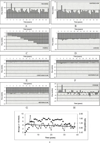
Simulated stream leakage showed sensitivity to the forcing terms set forth by recharge, prescribed eastern flow (Fig. 9b) and pumping (Fig. 9c). On the contrary, flux through con-stant head boundaries located to the west (Fig. 9e) and west-ern and southwest-ern boundary flows (Fig. 9f and g, respectively) were almost invariant over time and of comparable magni-tude, ranging between 155.2 hm3yr−1and 622 hm3yr−1 (5 to 20 m3s−1, respectively). Storage augments and decreases in response to sink/sources (Fig. 9h), but no clear trend can be identified. However, during the first years of exploitation, the combination of abundant recharge and low pumping pro-duces a rapid increase in cumulative storage (Fig. 9i). As pumping increases, cumulative storage stabilizes to decline rapidly towards the end of the simulation period, in tune with increasing pumping rates and low-recharge years. Declining recharge rates over time are illustrated by the straight line in Fig. 9i, representing the ratio between the recharge rate for thei-th year, REC(i) and the steady state recharge rate REC(SS).
The recent inventory of production boreholes in the GAS (Vives et al., 2008) resulted in a current groundwater ex-ploitation of about 1040 hm3yr−1. In global terms, the model water balance indicates that the current rate of groundwater withdrawals does not exceed the rate of recharge. Notwith-standing, pumping is concentrated in heavily populated and industrialized areas where groundwater withdrawals are ex-pected to continue rising in coming years; consequently, at
local scale the situation may be reversed, even at present. The regional model presented in this work did not intent to quantify local-scale issues. Local models already developed in critical areas would serve that purpose.
Table 3 shows budget terms for the years of maximum and minimum recharge as well as averages for the whole transient period. Recharge ranged from 2014 to 6470 hm3yr−1, aver-aging 3156 hm3yr−1, equivalent to 84.2 % of inflows. On av-erage, pumping totaled 665 hm3yr−1, representing 16.2 % of outflows. Part of the recharge is converted to leakage along streams. For the minimum recharge year, leakage constituted 53 % of outflows, reaching 70 % for the maximum recharge year, with an average of 61.4 %. Water is discharged through the aquifer boundaries, except at the eastern boundary. This result is consistent with the conceptual model. The magni-tude of the western flow plus the outward flow through con-stant heads to the west is comparable to pumping, while southern flows represent less than 10 % of outflows.
RECHARGE
0 75 150 225
0 3 6 9 12 15 18 21 24 27 30 33 36 Time (years) F lu x ( m 3 /s )
. EASTERN FLOW
0 25 50
0 3 6 9 12 15 18 21 24 27 30 33 36 Time (years) F lu x ( m 3 /s ) .
A B
PUMPING -50 -40 -30 -20 -10 0
0 3 6 9 12 15 18 21 24 27 30 33 36 Time (years) F lu x ( m 3 /s ) . LEAKAGE -225 -150 -75 0
0 3 6 9 12 15 18 21 24 27 30 33 36
Time (years) F lu x ( m 3 /s ) . C D
CONST.HEAD FLOW -50 -40 -30 -20 -10 0
0 3 6 9 12 15 18 21 24 27 30 33 36 Time (years) F lu x ( m 3 /s ) . SOUTHERN FLOW -50 -40 -30 -20 -10 0
0 3 6 9 12 15 18 21 24 27 30 33 36
Time (years) F lu x ( m 3 /s ) . E F
WESTERN FLOW -50 -40 -30 -20 -10 0
0 3 6 9 12 15 18 21 24 27 30 33 36 Time (years) F lu x ( m 3 /s ) . STORAGE -120 -80 -40 0 40 80 120
0 3 6 9 12 15 18 21 24 27 30 33 36
Time (years) F lu x ( m 3 /s ) . G H
[image:12.595.129.465.63.545.2]
I
Fig. 9. Model water budget components for zonation Z5. Flow rates are expressed in m3s−1, volumes are expressed in Hm3. Negative flows represent water out of the aquifer, positive flows represent water into the aquifer. (A), (B), (C), (D), (E), (F), (G) and (H): annual water budget terms; (I): cumulative storage (black circles), relative recharge (gray diamonds).
between 137 and 353 hm3yr−1; the simulated value for steady state was 335 hm3yr−1, augmenting during the tran-sient period. Notwithstanding the uncertainties and model limitations, this comparison contributes to building confi-dence in modeling results, helping to progressively close a water balance for the aquifer.
Recent calculations limit recharge to less than 10 % of mean annual precipitation, with values closer to 3–4 %. In a
Table 3. Model mass balance (volumetric rates expressed in
hm3yr−1, percentages referred to average rates) – PEF: prescribed
eastern flow; PH: prescribed head; WF: western flow; SF: south-ern flow. Maximum values correspond to the forth simulated year; minimum values correspond to the thirtieth simulated year.
Max Min Average %
Inflow Recharge 6470 2014 3516 84.2
PEF 1212 377 659 15.8
Total 7682 2391 4175 100
Outflow Leakage 3135 2155 2512 61.4
PH 194 149 164 4.0
WF 602 485 526 12.9
SF 293 191 227 5.5
Pumping 248 1024 665 16.2
Total 4472 4004 4094 100
Change in Storage 3210 −1613 81
Average stream leakage resulted 2512 hm3yr−1 (81 m3s−1) (in actuality, it ranged between 81 m3s−1 for Z5 zonation to 93.8 m3s−1for Z2 zonation). This result leads to two conclusions: firstly, stream/aquifer fluxes are not very sensitive to the number ofK zones; and secondly, total leakage is small in comparison to minimum flow discharges of the main rivers in the region. For example, the simulated average leakage for the Uruguay River was 8 m3s−1while the observed absolute minimum discharge for the period 1931/2001 was 382 m3s−1(its average discharge is 2300 m3s−1). This meager flow renders the verification of some modeling results very challenging.
Ara´ujo et al. (1999) postulated that the principal dis-charge area of the GAS was probably located between the Paran´a and Uruguay rivers, although Campos (2000) raised doubts about this hypothesis. Nonetheless, this hypothesis was tested with the model and proved to be consistent with the other water budget terms.
Distinct responses are found on a stream-by-stream basis analysis. Considering scenario 5 (Z5), all streams but num-bers 1, 3, 5, 11, 19 and 23 resulted influent (refer to Fig. 4 for streams identifications).
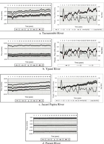
Four streams were selected in representative areas to study stream/aquifer fluxes in more detail: Tacuaremb´o River (out-cropping area in Uruguay, intensive pumping, Fig. 10a), Ypan´e River (outcropping area in Paraguay, low pumping, Fig. 10b), Jacar´e Papira River (outcropping area in north-eastern Brazil, very intensive pumping, Fig. 10c), and Paran´a River (confined area in northeastern Argentina, Fig. 10d).
In these four cases, stream/aquifer fluxes shown on the left of Fig. 10 were sensitive to changes in hydraulic con-ductivity. Streams located in heavily pumped regions, i.e. Tacuaremb´o River and Jacar´e Papira River, switched from a gaining condition in early years to a losing condition over
time for Z5 zonation. An auxiliary variable was defined for the analysis. Figure 10 shows the difference between leak-age for a particular year-Flux(i)- and leakage for steady state-Flux(SS)-. Transient recharge relative to steady state recharge, represented as a solid line, is also shown on the same figure. The Tacuaremb´o and Jacar´e Papira rivers show a similar behavior: flow from the river to the aquifer in-creases over time in response to increasing pumping. This situation has relevant connotations for conjunctive water re-sources management in localized areas of the aquifer and should be studied in more detail by combining field work to verify flow magnitudes and numerical simulations to predict system response under various scenarios. Recharge impacts leakage on the Tacuaremb´o River; however, it has little influ-ence on the Jacar´e Papira River. Recharge and pumping do not affect the stream/aquifer relationship in confined areas of the aquifer, represented in this case by the Paran´a River.
For those rivers, stream/aquifer fluxes for steady state, year 4 (maximum recharge year, minimum pumping), year 30 (minimum recharge year, average pumping), and last simu-lated year (close to average recharge, maximum pumping) were evaluated, comparing exchange fluxes with the cor-responding mean streamflow (Table 4). Leakage from the aquifer to the river decreases in the Jacar´e Pepira Stream due to increasing pumping. By the same token, leakage from the stream to the aquifer in the Ypan´e River increases slightly with time; however, that change is no so drastic due to rela-tively low pumping rates in the area. The simulated condition for the Tacuaremb´o River changes from effluent to influent though the leakage magnitude is small. There is no pump-ing in the area to justify this behavior. Finally, the interaction between the aquifer and the simulated reach of the Paran´a is negligible compared to the river mean discharge.
6.3 Hydraulic conductivity
For all zonations, K-values resulted from the automatic cal-ibration algorithm available in TRANSIN, minimizing an objective function written in terms of heads, parameters and concentrations (if a transport problem is solved). In TRANSIN, the minimizing algorithm uses the Marquardt Method, an iterative algorithm to solve non-linear problems for parameter estimation by the least square method.
Partitioning the model domain into an increasing num-ber of K zones was effective in improving the model fit, reducing calibration errors. However, calibrated K for all five scenarios were higher in the central region of the mod-eled area, with values above the conductivity range typi-cally expected for sandstones, even considering scale effects (Fig. 11). Along a central corridor and some adjacent ar-eas,K was always greater than 15 m d−1, even higher than 30 m d−1for scenarios Z2, Z4 and Z5, reaching a maximum of 114.8 m d−1for scenario Z2. The maximum calibratedK
-2.50 -1.25 0.00 1.25 2.50
0 2 4 6 8 10 12 14 16 18 20 22 24 26 28 30 32 34 36 38
Time (years)
F
lu
x
(
m
3
/s
)
.
Z1 Z2 Z3 Z4 Z5
a. Tacuarembó River
-2.50 2.50 7.50 12.50
0 2 4 6 8 10 12 14 16 18 20 22 24 26 28 30 32 34 36 38
Time (years)
F
lu
x
(
m
3
/s
)
.
Z1 Z2 Z3 Z4 Z5
b. Ypané River
-10.00 -5.00 0.00 5.00 10.00
0 2 4 6 8 10 12 14 16 18 20 22 24 26 28 30 32 34 36 38
Time (years)
F
lu
x
(
m
3
/s
)
.
Z1 Z2 Z3 Z4 Z5
c. Jacaré Papira River
-15.00 -12.00 -9.00 -6.00 -3.00 0.00
0 2 4 6 8 10 12 14 16 18 20 22 24 26 28 30 32 34 36 38
Time (years)
F
lu
x
(
m
3
/s
)
.
Z1 Z2 Z2 Z3 Z4
[image:14.595.131.466.60.523.2]d. Paraná River
Fig. 10. Left: stream/aquifer flux (m3s−1) versus time for selected streams for all conductivity zonations. Right: ratio of transient recharge
to steady state recharge (solid line – dimensionless) and change of stream/aquifer flux with respect to steady state condition (m3s−1) for all
conductivity zonations (the latter is not included for the Paran´a River because the magnitude of the change was negligible, i.e. less that 0,1
m3s−1, for all zonations).
the area, but they also would indicate the need for the model to conduct flows in that area through, for instance, a prefer-ential flow zone or a connection with overlying/underlying geologic units. This option should be explored in the future, incorporating a more detailed geologic layering and their hy-draulic interconnection to the conceptual model. Zones of low calibrated hydraulic conductivity along parts of the east-ern boundary and the northwest coincide with high hydraulic gradients.
Except for the homogeneous case, the lower end of the
K range was between 0.1 and 2.3 m d−1, a value coherent with sandstone K-values reported in the literature (Freeze and Cherry, 1979) and for the GAS.
Fig. 11. Calibrated hydraulic conductivity for alternative hydraulic conductivity zonations (yellow numbers on the lower-right map indicate:
1: Rivera/Santana area; 2: southern Paraguay; 3: Riberao-Preto area).
the model mesh is 25 km2), with K ranging from 0.17 to 19.92 m d−1, were available at the Uruguayan–Brazilian bor-der around the cities of Rivera/Santana (G´omez et al., 2010). Seven pumping tests, withKranging from 1.6 to 3.8 m d−1, were available in southern Paraguay (BGR, 2008). For the best model fit scenario, K for the zones overlaying those available point data were 5–10 m d−1(K22), and 2.5–5 m d−1 (K31), respectively, showing a good match between cali-brated and observed values.
Based upon eleven pumping tests, highly concentrated in space, hydraulic conductivity values of around 3 m d−1were reported for the Riberao Preto area in NE Brazil (Sracek and Hirata, 2002). Calibrated values for that area (K11) were in the range between 2.5 and 5 m d−1.
Besides the point-to-zone comparison, an attempt was made to compile ranges of reported K-values attributed to various authors that could be used to further assess the model calibration. Transmissivity (and for that matter hydraulic conductivity) is one of many aquifer parameters that vary with the scale of measurement. This issue is well documented in the literature (S´anchez-Vila et al., 1996; Nilsson et al., 2001). An in-depth analysis of this topic is well beyond the scope of this work. Nevertheless, given the spatial extent of the constructed model, a general comment is merited. This is the first, though not exhaustive, attempt to compile published values of hydraulic conductivity for GAS sandstones in the
four countries in order to assess the consistency of the model automatically calibratedKand identify spatial scale effects. Figure 12 shows the range of reported K-values compiled so far, attributed to various authors. Instead of the classical rep-resentation of logKvs. the scale of observation, the x-axis simply corresponds to a bibliographic reference number.
Depending on the use of packer tests, slug tests or pump tests, a clear scale effect in crystalline rocks, porous carbon-ate rocks and carboncarbon-ate aquifers was identified by Sanchez-Vila et al. (1996), Schulze-Makuch and Cherkauer (1998) and Whitaker and Smart (2000), respectively. For GAS sand-stones, there seems to be a scale dependence in hydraulic conductivity due to progressive incorporation of larger and better connected transmissive zones as the support volume increases. Reported K-values from aquifer test data show lit-tle variability. Available data sources do not provide enough information as to identify the test-type influence demon-strated by the aforementioned authors. Mean hydraulic con-ductivity for this data set is 2.15 m d−1, with reported mini-mum and maximini-mum values of 0.1 m d−1and 4.56 m d−1, re-spectively.
Table 4. Comparison between stream–aquifer fluxes with streamflow for selected streams and simulation years (percentages express stream
leakage relative to mean streamflow).
Observed
mean flow Simulated Steady state Year 4 Year 30 Last year
Stream (m3s−1) condition (%) (%) (%) (%)
Jacar´e Pepira (27) 29 Effluent −10.3 −14.2 −2.7 −2.4
Ypan´e (11) 94 Influent 3.3 2.5 3.7 3.3
Tacuaremb´o (23) 40.3 Effluent/influent −0.4 −1.7 1.4 0.8
Paran´a (20) 12 406 Efluent 0.0 0.0 −0.01 −0.01
R e fe re n c e n u m b e r
H
y
d
ra
u
li
c
c
o
n
d
u
c
ti
v
it
y
(m
/d
)
1 0-2 1 0-1 1 00 1 01 1 02
L o c a l sc a le A q u ife r te s t
L o ca l sc a le M o d e lin g
R e g io n a l s ca le M o d e lin g
1
2
3 4
5 6
7
8 9
1 0 1 1
1 2 1 3
1 4 1 5
1 6 1 7
1 8
1 92 0
[image:16.595.49.285.149.387.2]2 1
Fig. 12. Comparison between calibrated hydraulic conductivity and
hydraulic conductivity values compiled from bibliographic sources. The group “Local scale aquifer test” includes aquifer tests data; the
group “Local scale modeling” includes calibratedKfrom models
ranging from 100 km2to 5000 km2in extent; the group “Regional
scale modeling” includes calibratedKfrom models whose extent is
larger than 400 000 km2. Reference number 16 corresponds to the
model of the Paraguayan sector of the GAS; references 17–21
cor-respond to the five zonations discussed in this work.Kis reported
either as a single value or aKrange.
hydraulic conductivity and other parameters that may lead to non-unique modeling results (Scanlon et al., 2002). Hy-draulic conductivity and recharge rates are often highly cor-related; consequently, calibration based only on water level data is limited to estimating the ratio of recharge to hydraulic conductivity. Hence, as Scanlon et al. (2002) stated, the reli-ability of recharge estimates depends on the accuracy of the hydraulic conductivity data. Then, in many local scale mod-els aimed at estimating recharge rates, hydraulic conductivity values estimated from field data are considered rather repre-sentative while recharge rates are the main calibration pa-rameter (Rabelo and Wendland, 2009; Gomez et al., 2010), leading to “calibrated” K-values very similar to pump test values.
Table 5. Model structure identification based on the following
crite-ria implemented in TRANSIN: AIC (Akaike, 1974), BIC (Akaike,
1977), ø (Hannan, 1980) anddk(Kashyap, 1982).
#Kzones AIC BIC ø dk
Z1 1 4281 4285 4282 4289
Z2 9 4240 4275 4254 4285
Z3 17 4233 4300 4260 4314
Z4 19 4133 4209 4163 4221
Z5 31 4064 4188 4113 4229
As the size of the region of interest increases, calibratedK
also increases in both its magnitude and calibrated range. It should be pointed out that the Paraguayan groundwater flow model was based on a more detailed representation of geo-logic formations. GAS sandstones were simulated with two homogeneous layers, for which calibratedKwas 0.05 m d−1 and 3 m d−1, respectively; therefore, they should be consid-ered single values and not a hydraulic conductivity range (see dotted line in Fig. 12).
6.4 Model structure
[image:16.595.333.522.250.328.2]of the criteria themselves and their use in the context of TRANSIN, respectively.
Table 5 shows the values of each criterion for the different models. The Z5 zonation was the best model, mainly sup-ported by the large number ofK zones. Therefore, it is ex-pected to yield the best fit, even at the risk of model over-parametrization.
Increasing the number of zones decreases the values of the different criteria, suggesting that the definition of newK
zones is a consistent approach. Even though in the case of Z3 a better fit is achieved, the model is overparameterized. This is concluded from the values of ø and BIC, which allow see-ing the relationship between the number of parameters and the number of data. In contrast, with only two more zones, the Z4 model improves its predecessor, suggesting that zon-ing is defined consistently. This is reasonable because Z3 and Z4 zonings were defined using different sources of informa-tion and criteria (see Sect. 5.2).
7 Conclusions
Fresh water has already become a limiting resource in many parts of the world. In the future, it will become even more limiting due to increased population, urbanization, and cli-mate change. This limitation will be caused not just by in-creased demand for water, but also by pollution. Immersed within this context, the Guarani Aquifer System (GAS) is being increasingly exploited for freshwater supply, and for industrial and agricultural uses. In large aquifers, relevant for their considerable size, regional groundwater modeling remains challenging given geologic complexity and data scarcity in space and time. Yet, it may me conjectured that regional scale groundwater flow models can help in under-standing the flow system functioning and the relative mag-nitude of water budget components, which are important for aquifer management. The present study on the GAS has shown that a transient-regional scale groundwater flow model can provide valuable insights regarding those two is-sues, given an extraction volume still very small in compar-ison with the aquifer volume. Even though the model was constructed on a simplified conceptual model, it constitutes the first attempt to simulate the entire aquifer including bud-get terms previously overlooked.
The hypothesis of a continuous sedimentary unit may be sustainable as a first approximation to construct a numeri-cal model covering the full extent of the aquifer. Combined with an increasing number ofK zones and an appropriate set of boundary conditions, that hypothesis yielded errors within the calibration target in a regional sense. Nonetheless, this approach was insufficient to improve calibration in ar-eas known for the presence of structural controls that may influence groundwater flow patterns.
Given the amount and quality of data for calibration, model results were acceptable as measured by standard
statistics. Surely, the availability of current piezometric lev-els, extraction volumes and stream discharges would help to produce a better model.
Calibrated K-values were coherent, with low/high hy-draulic gradients. However, calibratedKin the central region of the modeled area was above the conductivity range typi-cally expected for sandstones. This result highlights the need to analyze the possible hydraulic interconnections between the GAS and pre-GAS/post-GAS sediments.
The location and character of the southwestern boundary of the aquifer remains an open issue, though it was demon-strated that reaches along the Paran´a and Uruguay rivers could be potential discharge zones, as postulated by previous authors. Simulated stream leakage along those reaches was very small, but so were other water budget components when analyzed in perspective considering the aquifer extent and its storage volume. The model was also instrumental for the un-derstanding of the dynamics of the system along the western boundary, which resulted in an outflow condition, compatible with observed water level data and hydraulic gradients. The magnitude of the simulated discharge through that boundary matched independent estimates by other researchers.
At a regional scale, the importance of the stream/aquifer interaction process was manifested by the 61.4 % contribu-tion of this term to total outflow, its magnitude being second to recharge. In addition, model-calculated recharge was co-herent with recent estimates from other studies. Even though an independent water budget for the entire aquifer is not yet available, these qualitative and quantitative analyses con-tribute to building confidence in model results.
On average, pumping represented 16.1 % of inflows while aquifer storage experienced a small overall increment. The model water balance indicates that the current rate of ground-water withdrawals does not exceed the rate of recharge in a regional sense. Notwithstanding, pumping is concentrated in heavily populated and industrialized areas where ground-water withdrawals are expected to continue rising in coming years; consequently, at local scale the situation may be re-versed, even at present. It is worth noting that this regional model did not intend to quantify local-scale issues. Local models already developed in critical areas would serve that purpose.
– Analyze the hypothesis of a compartmentalization of the aquifer and its influence on the regional flow sys-tem, as suggested by recent studies.
– Analyze the role of pre-GAS and post-GAS formations on piezometric levels and hence, on groundwater flows. – Evaluate the role of local geologic structures on the flow system. This would help to reproduce some piezometric (and hydrochemical) anomalies that could not be repre-sented by the current conceptual/numerical models. – Conduct more in-depth and model-independent
stud-ies of flows distribution especially related to recharge, pumping and river/aquifer interactions in outcropping areas, performing water balances at representative areas with sufficient field data to support hypotheses and con-clusions.
– Simulate groundwater age in order to validate alterna-tive hypotheses of the flow system functioning, sup-ported by isotopic sampling and analysis.
Acknowledgements. This work was financially supported by the
National Agency for the Promotion of Science and Technology PICT2008-2071 (Argentine), the Instituto de Hidrolog´ıa de Lla-nuras of the Universidad Nacional del Centro de la Provincia de Buenos Aires (Argentine), and the Facultad de Ingenier´ıa y Cien-cias H´ıdricas of the Universidad Nacional del Litoral (Argentine).
Edited by: J. Carrera
References
Akaike, H.: A new look at statistical model identification, IEEE T. Automat. Contr., 19, 716–722, 1974.
Akaike, H.: On entropy miximisation principles, in: Proc. Symp. on Applications of Statistics, edited by: Krishnaiah, P. R., 27–47, Amsterdam, The Netherlands, 1977.
Ara´ujo, L. M., Franca, A. B., and Poter, P. E.: Hydrogeology of the Mercosul Aquifer System in the Paran´a and Chaco-Paran´a Basins, South America, and comparison with the Navajo-Nugget Aquifer System, USA, Hydrogeol. J., 7, 317–336, 1999. Barthel, R.: An indicator approach to assessing and predicting the
quatitative state of groundwater bodies on the regional scale with a special focus on the impacts of climate change, Hydrogeol. J., 19, 525–546, 2011.
BGR: Uso sostenible del Sistema Acu´ıfero Guaran´ı en la Regi´on Oriental del Paraguay (Sustainable use of the Guaran´ı Aquifer System in the Oriental Region of Paraguay). Volumen 4 – Mod-elo de aguas subterr´aneas. Cooperaci´on t´ecnica Rep´ublica del Paraguay – Rep´ublica Federal de Alemania, 2008.
Bigarella, J. and Salamuni, R.: Early Mesozoic wind patterns as suggested by dune bedding in the Botucatu Sandstone of Brazil and Uruguay, Geol. Soc. Am. Bull., 72, 989–1106, 1961.
Bugeda, G.: Utilizaci´on de t´ecnicas de estimaci´on de error y gen-eraci´on autom´atica de mallas en procesos de optimizaci´on es-tructural, Escuela T´ecnica Superior de Caminos, Canales y Puer-tos de Barcelona, Universidad Polit´ecnica de Catalu˜na, Doctoral Thesis, Espa˜na, 1990.
Campos, H. C. N. S.: Applied groundwater modeling in the Bo-tucatu aquifer system, Brazil, 8th Congress of the International Association of Engineering Geology and the Environment, Van-couver, Canada, Proceedings Balkema, Rotterdam, 2359–2366, 1998.
Campos, H. C. N. S.: Mapa hidrogeol´ogico do aqu´ıfero Guarani, Acta Geol. Leopoldensia, 23, 1–50, 2000.
Carrera, J. and Neuman, S.: Estimation of aquifer parameters un-der transient and steady state conditions, I, Maximum likelihood method incorporating prior information, Water Resour. Res., 22, 199–210, 1986.
Carrera, J., Alcoleta, A., Medina, A., Hidalgo, J., and Slooten, L.: Inverse problem in hydrogeology, Hydrogeol. J., 13, 206–222, 2005.
Chang, H.: Protec¸˜ao Ambiental e Gerenciamiento Sustent´avel In-tegrado do Aq¨u´ıfero Guaran´ı- tema 3 (Environmental protection and sustainable management of the Guaran´ı Aquifer, topic 3), available at: http://www.ana.gov.br/guarani/gestao/gest cbasico. htm (last access: August 2012), UNESP/IGCE, Sao Paulo, 2001. Custodio, E. and Llamas, J. R.: Hidrolog´ıa Subterr´anea, Omega,
Barcelona, 2450 pp., 1976.
Fernandes, A. J., Wahnfried, I., Varnier, C., Maldaner, C., Pressinotti, M. M. N., Ferreira, L. M. R., Iritani, M. A., Hi-rata, R., Shapiro, A., and Rouleau, A.: Modelo conceitual de circulac¸˜ao de ´agua nos basaltos de Ribeir˜ao Preto e como isto afeta a vulnerabilidade do SAG, in: SODERMA, Congr. Aqu´ıfero Guarani, 2, Ribeir˜ao Preto, Anais (CD-ROM), 6 pp., 2008.
Fernandes, A. J., Negri, F., Azevedo Sobrinho, J. M., Varnier, C., and Janasi, J.: Analise de fraturas dos basaltos do Aquifero Serra Geral e o potencial de recarga regional do Sistema Aquifero Guarani, Bolet´ın Geol´ogico y Minero, 123, 325–339, 2012. Ferreira, F. J. F.: Alinhamentos estruturais-magn´eticos da regi˜ao
Centro-Oriental da Bac´ıa do Paran´a e seu significado tectˆonico, Geolog´ıa da Bac´ıa do Paran´a, Reavaliac¸˜ao da Potencialidade e Prospectividade em Hidrocarbonetos, Sao Paulo, PAULIPETRO, 143–166, 1982.
Foster, S., Hirata, R., Vidal, A., Schmidt, G., and Gardu˜no, H.: The Guaran´ı Aquifer initiative – towards realistic groundwa-ter management in a transboundary context, GW-Mate Sustain-able Groundwater Management, Lessons for Practice, Case Pro-file Collection No. 9, available at: http://water.worldbank.org/ gwmatepubs (last access: August 2012), 2009.
Freeze, R. A. and Cherry, J. A.: Groundwater., Prentice Hall, En-glewood Cliffs, NJ, 1979.
Gastmans, D., Veroslavsky, G., Kiang Chang, H., Caetano-Chang, M. R., and Nogueira Pressinotti, M. M.: Modelo hidrogeol´ogico conceptual del Sistema Acu´ıfero Guaran´ı (SAG): una her-ramienta para la gesti´on, Bolet´ın Geol´ogico y Minero, 123, 249– 265, 2012.