ScholarWorks @ Georgia State University
ScholarWorks @ Georgia State University
Computer Science Theses Department of Computer Science
Summer 7-15-2010
A Novel Stable Model Computation Approach for General
A Novel Stable Model Computation Approach for General
Dedcutive Databases
Dedcutive Databases
Komal Khabya
Georgia State University
Follow this and additional works at: https://scholarworks.gsu.edu/cs_theses
Recommended Citation Recommended Citation
Khabya, Komal, "A Novel Stable Model Computation Approach for General Dedcutive Databases." Thesis, Georgia State University, 2010.
https://scholarworks.gsu.edu/cs_theses/68
This Thesis is brought to you for free and open access by the Department of Computer Science at ScholarWorks @ Georgia State University. It has been accepted for inclusion in Computer Science Theses by an authorized
administrator of ScholarWorks @ Georgia State University. For more information, please contact
A NOVEL STABLE MODEL COMPUTATION APPROACH FOR GENERAL DEDUCTIVE
DATABASES
by
KOMAL KHABYA
Under the Direction of Rajshekhar Sunderraman
ABSTRACT
The aim of this thesis is to develop faster method for stable model computation of
non-stratified logic programs and study its efficiency. It focuses mainly on the stable model and weak
well founded semantics of logic programs. We propose an approach to compute stable models by
where we first transform the logic program using paraconsistent relational model, then we
compute the weak-well founded model which is used to generate a set of models consisting of
the true and unknown values, which are tested for stability. We perform some experiments to test
the efficiency of our approach which incurs overhead to eliminate negative values against a
Naïve method of stable model computation.
DATABASES
by
KOMAL KHABYA
A Thesis Submitted in Partial Fulfillment of the Requirements for the Degree of
Master of Science
in the College of Arts and Sciences
Georgia State University
Copyright by Komal Khabya
DATABASES
by
KOMAL KHABYA
Committee Chair: Rajshekhar Sunderraman
Committee: Sushil Prasad
Yanqing Zhang
Electronic Version Approved:
Office of Graduate Studies
College of Arts and Sciences
Georgia State University
ACKNOWLEDGEMENTS
I would like to thank my parents and my family for being the constant source of
encouragement during my life. Their motivation and support have always been there for me.
I am indebted to my advisor Dr. Rajshekhar Sunderraman for teaching me about the
interesting field of deductive databases and logic programming. His motivational words and the
guidance throughout have helped me achieve my goals. His ability to work hard and patience
inspires me and would keep inspiring other students. He has been a friend, philosopher and guide
through all the good and bad days. He has given me confidence and made me grow into a better
person. I would also like to thank my committee members Dr. Sushil Prasad and Dr. Yanqing
Zhang for giving their valuable time and assessing my work.
I am thankful to God Almighty for giving me the strength and for being kind to me at
every step, and enlighten me to take the right course of path.
I am also thankful to my friends here at Georgia State who were there for me to share my
problems and help me in every way they can. Last but not the least; I am thankful to my husband
for being there for me and supporting me throughout this time.
TABLE OF CONTENTS
ACKNOWLEDGEMENTS ...iv
LIST OF TABLES ... viii
LIST OF FIGURES ... ix
1. INTRODUCTION... 1
I BACKGROUND ... 3
2. DEDUCTIVE DATABASES AND LOGIC PROGRAMMING ... 4
2.1 Introduction ...4
2.2 Logic Programs ...5
2.2.1 Definite Logic Programs ...6
2.2.2 Model Theoretic Semantics ...6
2.2.3 Fix-Point Semantics ...8
3. NEGATION ...11
3.1 Introduction ...11
3.2 Stratified Logic ...12
3.3 3-Valued Semantics ...14
3.3.1 Fitting’s Semantics ...15
3.3.2 Well Founded Semantics and Unfounded Sets ...17
3.4 Stable Model Semantics ...19
4. PARACONSISTENT RELATIONAL DATAMODEL ... 23
4.1 Paraconsistent Relations ... 23
4.2 Formal Definition of Paraconsistent Relations ... 23
II A NOVEL APPROACH FOR STABLE MODEL COMPUTATION ... 27
5. THE PROPOSED APPROACH ... 28
5.1 Assumptions ... 28
5.2 Overview of the Steps Involved ... 29
5.3 Modules ... 30
5.3.1 Datalog Compiler ... 30
5.3.2 Transformation ... 33
5.3.3 Fitting’s Model Generation ... 46
5.3.4 Models and Ground Program Generation ... 48
5.3.5 Stable Model Tester ... 50
5.4 Implementation of the Modules ... 52
5.4.1 Compiler ... 52
5.4.2 Generating Transformed Program ... 54
5.4.3 Fitting’s Model Generation ... 56
5.4.4 Models Generation ... 57
5.4.5 Stable Model Tester ... 58
6. EXPERIMENTS ... 60
6.1 Introduction ... 60
6.2 Design of Experiments ... 60
6.3 Results ... 63
6.4 Analysis of Result ... 66
7. CONCLUSION ... 67
9. APPENDIX: Java code used to implement our approach ... 72
9.1 Lexer ... 72
9.2 Parser ... 73
9.3 Predicate Class ... 75
9.4 Rule Class ... 76
9.5 Main Class ... 77
9.6 Semantics Checks Class ... 79
9.7 Transformation Class ... 82
9.8 Weak Well Founded Model ... 91
9.9 Generate Models for Stability Testing ... 96
9.10 Ground Program Generation ... 97
LIST OF TABLES
Table 5.1 Predicate...31
Table 5.2 Rule ...32
Table 5.3 Fix point computation for predicate t ...47
Table 6.1 Results from Experiment 1 ...55
LIST OF FIGURES
Figure 3.1 Dependency graph for example 3.1.1 ...13
Figure 5.1 Block diagram for the proposed approach...30
Figure 5.2 Circuit for example 5.2.2 ...36
Figure 5.3 Paraconsistent expression tree ...39
Figure 5.4 Named paraconsistent tree ...40
Figure 5.5 Tree for expression 1 ...44
Figure 5.6 Tree for expression 2 ...44
Figure 5.7 Block diagram for compiling process...52
Figure 6.1 Comparison of our approach with naïve approach in terms of steps involved ...63
Figure 6.2 Naïve approach vs. our approach with variable number of facts ...64
CHAPTER 1
INTRODUCTION
Deductive databases and logic programming have been widely recognized as expressive
knowledge representation formalisms. One can draw inferences firstly based on a database and
secondly by applying a set of rules to infer more information based on the information in the
database. For example it is given that man (Socrates) and mortal(X):- man(X) then based on the
information that Socrates is man and applying the rule we get mortal (Socrates). According to
closed world assumption if certain fact is not derivable from the database with any of the
inference rules it is assumed to be false, for example if the database has no other rules like
man(Thor) then infer ¬man(Thor). Negation as failure is not true in classical logic, but it is an
assumption made in traditional databases, i.e. if database does not contain information that
Socrates is manger of Department of Sales then assumes he is not, but what if the information is
not yet available then the appropriate answer would be unknown.
There has been a continuing research on the correct semantics of logic programs. The
idea of using first order predicate logic as a programming language was introduced by van
Emden and Kowalski in [1]. In this paper they provide semantics for class of logic programs
called the Horn programs. A number of extensions were found to be necessary in order to gain
expressivity. Initially, the Horn logic programs were extended to include negation in the body of
rules. Clark [2] proposed a notion of a completion of a logic program, a notion developed further
by Shepherdson [3, 4]. Fitting [5] and Kunen [6] developed this into the 3-valued theory. These
are some of the semantics that have emerged as being the most widely accepted by research
community which gave more uniform semantics by interpreting the program completion in
founded [5], well founded model [7] and the stable model semantics [8]. Research has shown
that these semantics have higher expressible power than some of the other semantics mentioned
above.
This thesis focuses mainly on the stable model and weak well founded semantics of the
logic programs. It has been motivated by our efforts to develop faster algorithms to compute
stable models. The outline of the thesis is as follows. Chapter 2 is an introduction to deductive
databases and logic programming focusing mainly on definite logic programs and its semantics.
In Chapter 3 we introduce negation in logic programs, its types and the 3-valued semantics of
general logic programs i.e. the weak well founded, well founded and stable model semantics.
Chapter 4 goes over the paraconsistent data model, a data model based on the open world
assumption. We introduce an algorithm for transforming the logic program consisting of harmful
negation into harmless negation using paraconsistent data model. In part 2 we introduce our
approach for faster stable model computation. In chapter 5, we propose our approach for stable
model computation which goes through the assumptions and the actual processes involved. We
first transform the original logic program into another logic program using paraconsistent data
model. Then we compute the Fitting‟s model of the program that gives us the true, false and
unknown values. Using the true and unknown values we generate possible sets of models that are
tested for stability. We also generate stable models using the Naïve approach. In chapter 6, we go
over the experiments conducted to compare the results and efficiency of our approach i.e., using
Fitting‟s model with a Naïve method. The time taken to compute the stable models is taken
under consideration, and the efficiency of the two methods is compared. The results show that
Part I
CHAPTER 2
DEDUCTIVE DATABASES AND LOGIC PROGRAMMING
2.1 Introduction
In recent years deductive databases have been an area of intense research which has brought
dramatic advances in the field of theory, systems and applications. A salient feature of deductive
databases is their capability of supporting a declarative, rule-based style of expressing queries
and applications on database. Relational databases, which are lacking in built-in reasoning
capabilities, have also demonstrated the desirability of using a declarative logic-based
language. Therefore deductive databases provide a declarative, logic based language for
expressing queries, reasoning and complex applications on databases [23].
Research on deductive databases has also contributed to areas such as non-monotonic
reasoning and knowledge representation by extending the declarative semantics of Horn Clauses
(based on the concepts minimal model and least-fixpoint [10, 11]) to non-monotonic constructs
such as negation and sets. Concepts, such as stratification [9], well-founded models, and
stable models have shed new light on various aspects of non-monotonic reasoning and
knowledge representation, and have also provided formal semantics to seemingly unrelated
concepts such as non-determinism [12]. Many of these theoretical contributions had a practical
impact, current deductive database systems provide efficient support for stratified negation; work
is progressing on finding efficient ways to support more powerful semantics (e.g., well-founded
models).
A deductive database is commonly viewed as a general logic program. A general logic
database consist of EDB (extensional database) rules known as facts that sit above the IDB
(intentional database) rules. The IDB rules are evaluated using the EDB in a recursive manner to
give the meaning of the program. The example taken from [13], shown next consists of three
EDB rules and two IDB rules.
Example 2.1.1
t0(2).
g(2, 3, 4).
g(3 ,4, 5).
g(5, 1, 3).
t(Z) ← t0(Z).
t(Z) ← g(X, Y, Z), t(X), not t(Y).
Before going into details of the semantics of general logic programs, we go through the
background of logic programs without negation and its semantics.
2.2 Logic Programs
Logic programs have emerged as a very expressive tool for knowledge representation. It is
programming by description which uses logic to represent knowledge and uses deduction to
solve problems by deriving logical consequences. We introduce the basic concepts of logic
programming and focus mainly on the declarative semantics of logic programs. These semantics
include the model theoretic and fix point semantics. The reader is referred to [11] for a more
2.2.1 Definite Logic Programs
We now introduce definite logic programs that are logic programs without negation. A definite
logic program is a set of Horn Clauses. Before defining Horn clause we look into some basic
structures.
A term is either a variable or an expression f(t1, t2,... tn) where f is the function symbol and ti are
terms. Constants are 0-ary function symbols. An atom of the language is of the form P(t1,
t2,…,tn) or negation of P(t1, t2,…,tn) where P is the predicate symbol with finite arity n ≥0 and
t1,…, tn are terms. A literal is either an atom or its negation denoted by p(t1, t2…, tn).
A definite logic program is a set of rules of the form
A ← B1, B2 …, Bn
Where A, B1, B2,…, Bn are atoms. Here A is called the head or conclusion of the rule and
conjunction of B1 ʌ B2 ʌ …ʌ Bn is called the body or premise of the rule. We now describe the
model theoretic and fixpoint semantics of logic programs.
2.2.2 Model Theoretic Semantics
This is the declarative semantics of the logic program that describes the meaning of a logic
program in terms of the set of models of the program viewed as a logical theory. To determine
the set of models of a logic program, we can use the work of Herbrand, who showed how to
define models from given theories, and showed that any consistent theory always has a model,
which is denumerable. This is the theory‟s Herbrand model. To determine the Herbrand model,
we first construct the Herbrand universe of the logic program. For a logic program P the
constants and function symbols occurring in the program P. A term, atom, literal, rule or
program is ground if it is free of variables. A ground instance of a rule is obtained by replacing
the variables in a program with elements from Up in every possible way. A ground program is
the union of the ground instances of the rules in the program. An example of Herbrand universe
of a logic program is shown below.
Example 2.2.2
Consider a logic program as
natural_number(0).
natural_number (s(X)) ← natural_number(X).
Here the set of constants is {0} and set of function symbols is {s}. Thus the Herbrand universe is
{0, s(0), s(s(0)),…….}. If there are no function symbols we get a finite Herbrand universe. So,
the Herbrand universe is the set of all possible terms that the theory can make assertions about.
The Herbrand base of P, denoted by HBp, is the set of all possible ground atoms whose predicate
symbols occur in P and whose arguments are elements of Up. For example for the Herbrand base
of above program is
{natural_number(0), natural_number(s(0)), natural_number(s(s(0))), … }
Herbrand Interpretation I of P is any subset of the Herbrand base of P. It is an assignment of
truth or falsity to each element of Herbrand base. For the natural number example the entire
Herbrand base must be assigned true. A Herbrand interpretation simultaneously associates, with
1. A ground atomic formula A is true in a Herbrand interpretation I iff A ∈ I.
2. A ground negative literal ¬A is true in iff A ∉I.
3. A ground clause L1 V L2 V…V Lm is true in I iff at least one literal Li, is true in I.
4. In general a clause C is true in I iff every ground instance C𝜎 of C is true in I. (C𝜎 is
obtained by replacing every occurrence of a variable in C by a term in UP. Different
occurrences of the same variable are replaced by the same term.)
5. A set of clauses A is true in I iff each clause in A is true in I.
A literal, clause, or set of clauses is false in I iff it is not true. If A is true in I, then we say that I is
a Herbrand model of A. Let M(A) be the set of all Herbrand models of A; then ∩M(A), the
intersection of all Herbrand models of A, is itself a Herbrand interpretation of A. This holds for
any set of clauses A even if A is inconsistent. If A is a consistent set of Horn clauses then
∩M(A) is itself a Herbrand model of A. More generally, Horn clauses have the model
intersection property: If L is any nonempty set of Herbrand models of A then ∩L is also a model
of A, and is the least such model of A which are the declarative semantics of logic programs. For
details refer to [1].
2.2.3 Fix-Point Semantics
The least model semantics provide logic based declarative definition of the meaning of a
program. We need to now consider constructive semantics and effective means to realize the
minimal model semantics. A constructive semantics follows from viewing the rules as
constructive derivation patterns, whereby, from the tuples that satisfy the patterns specified by
customary to consider the mapping TP called the Immediate Consequence Operator, for P,
defined as follows:
TP (I) = {A | A :- B1, B2, …, Bn∈ ground(P) and {B1, B2, …, Bn} ⊆ I }
TP(I) contains a ground atomic formula 𝐴 ∈𝐻𝐵𝑝 iff for some ground instance 𝐶𝜎 of a clause C
∈ P, C𝜎 = A ← B1, B2, …, Bn∈ ground(P) and {B1, B2, …, Bn} ⊆ I, n ≥ 0. Thus TP is a mapping
from Herbrand Interpretations of P to Herbrand Interpretations of P.
The least fixpoint computation amounts to an iterative procedure, where partial results
are added to a relation until steady state is reached. The least fixpoint of TP is the least model
of P. This result relies on the fact that TP is monotonic and hence posses a least fixpoint. TP is
monotonic means for any interpretations I1and I2 such that I1⊆ I2 then TP (I1) ⊆ TP (I2). The least
fixpoint is given by:
∩{I: TP(I) ⊆ I}
For a definite logic program P let M(P) be its Herbrand Models and let ∩M(P) be its least
model. Let C(P) be set all interpretations closed under TP, i.e., I ϵ C(P) iff TP(I) ⊆ I. We need to
show that ∩M(P) = ∩C(P). It is easier to show that M(P) = C(P).
Theorem 1.2.1 If P is a definite logic program then M(P) = C(P), i.e. |=I P iff T(I) ⊆ I, for all
Herbrand Interpretation I of P.
Proof. (|=I P implies TP(I) ⊆ I). Suppose I is a model of P, we want to show that if A ∈ TP(I) then
A ∈ I. Assume that A ∈ TP(I). Then by definition of TP there is a clause C ∈ P such that C𝜎 = A
← B1, B2, …, Bn, where B1, B2, …, Bn∈ I. Since I is a model of P, C𝜎is true in Iwhich means
(TP (I) ⊆I implies |=I P).Suppose that I is not a model of P. Then for some
clause C ∈ P, C𝜎 = A ← B1, B2, …, Bnis false in I, i.e., B1, B2, …, Bn∈ Iand A ∉I. But by
definition of TP, since B1, B2, …, Bnϵ I, A ∈ TP(I). Thus TP⊈ I.
It can also be shown that the least model is the limit of the increasing, possibly infinite
sequence of iterations ∅, TP(∅), TP(TP(∅)),…. There is a standard notation used to denote
elements of the sequence of interpretations constructed for P. Namely:
TP ↑ 0 = ∅
TP ↑ i+1 = TP (TP ↑ i)
TP ↑ 𝜔 = ∞𝑖=0𝑇𝑝 ↑ 𝑖
We show the iterations of TP operator with an example.
Example 2.2.2 Consider the definite logic program
odd (s(0)).
odd (s(s(X))) :- odd(X).
TP ↑ 0 = ∅
TP ↑ 1 = {odd(s(0))}
׃
TP ↑ 𝜔 = {odd (sn(0) | n ϵ {1, 3, 5,…}}
In conclusion the least fix point approach and least model approach assign the same meaning to a
CHAPTER 3
NEGATION
3.1 Introduction
In this chapter we describe some of the results in extending Horn clause programs to
include negation in the body of clauses. Such logic programs are called general logic programs
or normal logic programs. A normal logic program is a finite set of normal clauses. A normal
clause is a rule of the form:
A ← B1, B2…Bn, ~C1…~Cm
where, A is an atom and B1,…Bn and C1,…Cm are literals. When we have a collection of Horn
clauses (rules without negation) , then we know there is a unique minimal model of the program
that assigns the meaning to the program. However these types of rules are often too limited in
covering the expanse of queries that could be answered. But, as soon as we introduce negation in
the rules there is no guarantee of a unique minimal and in fact, it is normal to have more than one
minimal model. This can be illustrated from an example from [13]. There are two bus lines from,
red and blue, which runs between pairs of cities. Predicate blue(X, Y) is true if blue line runs a
bus from city X to city Y, while red(X, Y) has corresponding meaning for red line. The president
of red line wants to find out where red has monopoly, i.e. a pair of cities such red runs bus
between them, but on blue buses you cannot even travel from X to Y through a sequence of
intermediate cities. Suppose the data relation for both blue and red are blue(1, 2), red(1, 2) and
Example 3.1.1
(1) bluePath (X, Y) ← blue (X, Y).
(2) bluePath (X, Y) ← bluePath (X, Z), bluePath (Z, Y).
(3) monopoly (X, Y) ← red (X, Y) , not bluePath (X, Y).
The above program has two minimal models (A):{bluePath (1, 2), monopoly (2, 3)} and
(B):{bluePath (1, 2), bluePath (2, 3) , bluePath (1, 3)}, both having the EDB rules. The first
model makes sense the only bluePath is one that follows from Rule 1 and monopoly fact follows
from Rule 3, but the second model makes no sense and the facts bluePath(2, 3) and bluePath(1,
3) seems to appear from nowhere. However it is also a minimal model, in that
1. When you make any substitutions of constants for X, Y and (if necessary) Z, rules (1) –
(3) are true if the true ground atomic formulas are those given in (B), plus the given data.
2. If we delete one or more facts from (B), point (1) no longer holds.
But the question is which one is the intended model of the program, and the first model seems to
be the intended one.
3.2 Stratified Logic
The least controversial type of negation is stratified negation, where there is no recursion
involved in negated subgoals. This idea was arrived at by Van Gelder [14], Apt, Blair and
Walker [9], and Naqvi [15]. A normal logic program P is stratified if there is an assignment of
integers (0, 1, 2…3) to predicates p in P such that for each clause r in P the following holds. If p
is the predicate in head of r and q is the predicate Li in body of r then stratum (p) ≥ stratum (q),
as monopoly depends negatively on bluePath but bluePath does not depend at all on monopoly,
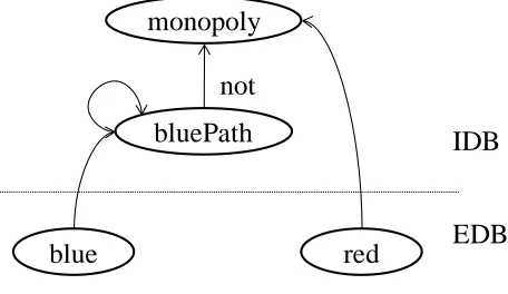
i.e. there are no cycles with negation. We can draw a dependency graph for the above logic
program to check whether it is stratified or not. The dependency graph which does not involve
cycles with not, depicts a stratified logic program. The EDB predicates are drawn lowest while
the IDB predicates are drawn higher, and if there is a rule p :- q then p is drawn above q. For the
[image:24.612.188.416.250.382.2]above logic program the dependency graph is as follows:
Figure 3.1 Dependency graph for example 3.1.1
So, we can compute bluePath facts completely from Rules (1) and (2) and then use Rule (3) to
compute monopoly facts. This process yields the first model {bluePath(1, 2), monopoly (2, 3)}
for the example above and confirms that this should be the intended model. The result of
computing predicates this way is often known as the perfect model which is defined by taking
least fixed point in order from lower strata to higher strata. An alternative view is
circumscription [16], of dealing with negation that says the only facts true for predicates are
those that can be followed from rules and given data. Then for example 3.1.1 we circumscribe
bluePath and declaring those facts as true that follow from rules (1) and (2) and given blue data,
and declaring all other pairs of X, Y for bluePath as false. Then these facts are used in rule (3) to
assert monopoly facts.
blue red
monopoly
bluePath
The idea of stratification was extended Przymusinska and Przymusinski [17] into locally
stratified programs. Here the predicate can negatively depend on itself, but when rules are
instantiated by constants the program contains no cycles. A program can be locally stratified for
one set of EDB rules and non- stratified for another. The semantics of locally stratified
programs have been treated in [14, 9, 17, 18] where they give a definition of perfect models and
have shown that locally stratified programs have one. An example of locally stratified program is
given next, which represents a board game that says a player wins the game if board is on
position X and there is a legal move from X to Y and Y is not a winning position.
Example 3.2.1
win(X) ← move(X,Y) , not win(Y).
Here win depends negatively on itself, so it is not stratified. However if move is acyclic i.e., you
can move from X to Y but there is no sequence of moves that takes you from Y to X. Then if we
instantiate the rules in all possible ways, there is no way win(a), for a particular board game a,
can depend negatively on itself, Thus, win rule is locally stratified provided move is acyclic.
Next, we present the semantics of non-stratified programs.
3.3 3-Valued Semantics
The landmark paper of Fitting [5] introduced semantics for logic programs with negation that
was very different and gave a more uniform semantics, based on the 3-valued logic given by
Kleene. The 3rd truth value, connotes unknown truth value, thus now an atom can be possibly
true, false, or unknown. A principal result was that every program has a minimum 3-valued
model and that according to Fitting could be taken as the semantics of the program from now on
thrust to provide meaning of non-stratified program is the well founded model of van Gelder, ross
and Schilpf [7].We briefly describe here the Fitting‟s semantics and the well founded semantics.
3.3.1 Fitting’s Semantics
Fitting‟s semantics is based on the notion of partial interpretations. We give a brief
description here, the reader is referred to [5] for detailed information.
Definition 1. A partial interpretation is a pair 〈I+, I-〉, where I+ and I- are any subsets of the
Herbrand base.
A partial interpretation is consistent if I+ ∩ I- =∅. For any partial interpretations I and J
we let I ∩ J be the partial interpretations 〈I+∩ J+, I-∩ J-〉 , and I ∪ J be the partial interpretations
〈I+ ∪ J+, I- ∪ J-〉. We also say that I ⊆ J, whenever I+⊆ J+ and I-⊆ J-. The Fitting‟s model for a
general logic program P is the least fixed point of the immediate consequence function 𝑇𝑃𝐹 on
consistent partial interpretations defined as follows (let P* be the ground version of P):
Definition 2. Let I be the partial interpretation, then 𝑇𝑃𝐹 (I) is the partial interpretation given by
𝑇𝑃𝐹 (I+) = {a | for some clause a ← l1, l2… lm∈ P*, for each 1≤ i ≤ m
if li is positive li∈ I+ and,
if li is negative li′ ∈ I-}
𝑇𝑃𝐹 (I-) = {a | for some clause a ← l1, l2… lm∈ P*, for each 1≤ i ≤ m
if li is positive li∈ I- and,
where li′ is the complement of literal li. It is easily seen that 𝑇𝑃𝐹 is monotonic and its application
on consistent partial interpretation results in consistent partial interpretation. It thus poses a least
model that is the Fitting model for P. This least fixed point is easily shown to be 𝑇𝑃𝐹↑ 𝜔, where the ordinal powers of 𝑇𝑃𝐹are defined as follows:
Definition 3. For any ordinal α,
〈∅, ∅〉 if α = 0,
𝑇𝑃𝐹↑ α = 𝑇𝑃𝐹 (𝑇𝑃𝐹 ↑ (α -1)) if α is a successor ordinal,
〈∪β<α(𝑇𝑃𝐹 ↑ β)+, ∪β<α(𝑇𝑃𝐹 ↑ β)- 〉 if α is limit ordinal
We show an example of Fitting semantics computation on a general deductive database.
Example 3.3.1 Consider a general deductive database P :
r(a, c).
r(b, b).
s(a, a).
p(X) ← r(X, Y) , not p(Y).
p(Y) ← s(Y, a).
Then 𝑇𝑃𝐹 ↑ 0 = 〈∅, ∅〉. 𝑇𝑃𝐹 ↑ 1 is given by the following partial interpretation:
(𝑇𝑃𝐹 ↑ 1)+ = {r(a, c), r(b, b), s(a, a)},
s(a, b), s(a, c), s(b, a), s(b, b), s(b, c),
s(c, a), s(c, b), s(c, c)} .
And 𝑇𝑃𝐹 ↑ 2 = I ∪ 𝑇𝑃𝐹 ↑ 1, where I is the partial interpretation 〈{p(a)},{p(c)}〉. Furthermore, for every ordinal α > 2, 𝑇𝑃𝐹 ↑ α can be seen to be same as 𝑇
𝑃𝐹 ↑ 2. So, we can see in
Fitting‟s model that it assigns p(a) as true, p(c) as false and no truth value is assigned to p(b).
Fitting‟s semantics has the distinction of being the first semantics to provide unique model for
general logic programs. However, they fail to capture positive recursion.
Example 3.3.2: Consider the following logic program:
a(0) ← b(0).
b(0) ← a(0).
The Fitting‟s model for this program is 〈∅, ∅〉, and it assigns truth value unknown to both a(0)
and b(0). It is easily seen that there is positive recursion between a(0) and b(0). This is captured
by the well founded semantics.
3.3.2 Well Founded Semantics and Unfounded Sets
The well founded semantics are also the 3-valued semantics given by Van Gelder et al. It
assigns some ground atoms truth value as true, some as false and rests are unknown. The
unfounded sets form the basis of negative conclusions in well founded semantics. For detailed
Definition 4. Let a program P, its Herbrand base H and a partial interpretation I be given. Then
A ⊆ H is an unfounded set of P with respect to I if each atom p ∈ A satisfies the following
condition: For each instantiated rule r of P whose head is p, (at least) one of the following holds.
1. Some positive subgoal q or negative subgoal not q of body occurs in ¬I i.e., is
inconsistent with I.
2. Some positive subgoal of body occurs in A.
Informally the well founded semantics uses condition (1) and (2) to draw negative conclusions.
We illustrate unfounded sets through example 3.3.3.
Example 3.3.3
Consider thefollowing ground logic program:
p(a) ← p(c), not p(b).
p(b) ← not p(a).
p(e) ← not p(d).
p(c) ← .
p(d) ← q(a), not q(b).
p(d) ← q(b), not q(c).
q(a) ← p(d).
q(b) ← q(a).
The atoms {p(d), q(a), q(b), q(c)} form the unfounded set with respect to interpretation ∅. q(c)
satisfies the first condition and p(d), q(a) and q(b) satisfy the second condition. It is easily seen
that p(d), q(a) and q(b) depend positively on each other. As a result none of them can be the first
to be proven true. Also declaring one of them false does not make any other remaining two true.
each other. This is because they depend negatively on each other. As a result making one of them
false makes the other true. And if both are declared false at once we have inconsistency. The
intuition of preceding example is immediate that union of arbitrary unfounded sets is an
unfounded set. This leads naturally to:
Definition 5. The greatest unfounded set of P with respect to I, GUSP(I) is the union of all
unfounded sets with respect to I.
We now define three transformation needed to in turn define the well founded partial
model.
Definition 6. The transformations TP(I), UP(I) and WP(I) are defined as follows:
TP(I) is the transformation defined by p ∈ TP(I) if and only if there is some instantiated
rule r of P such that r has head p, and each subgoal literal in body of r occurs in I.
UP(I) is the transformation defined by UP(I) = ¬G, where G is GUSP(I).
Finally WP(I) = TP(I) ∪ UP(I).
Definition 7. The well founded semantics of a program P is the least fixed point of WP(I). Every
positive literal denotes that its atom is true, every negative literal denotes that its atom is false
and missing atoms have undefined truth value.
3.4 Stable Model Semantics
Another competing thrust that provides meaning to general logic programs is the stable
model semantics. They were proposed by Gelfond and Lifschitz [8] at around the same time as
In its original form it is a two-valued semantics that is every atom is either true or false.
The notable feature of stable model semantics is its simplicity. We first define stable models for
logic programs without negation i.e., definite logic programs.
Definition 8. The least model of a definite logic program is the smallest set of atoms M such that
for every rule of the form
A ← B1, B2, …, Bn.
If B1, B2, …, Bn∈ M then A ∈ M.
This definition is same as TP for definite logic programs as defined by Emden and Kowalski.
Thus for general logic program the stable model is a set of atoms. We assume that a set of atoms
is available to us and based on certain transformations we decide whether the given set is stable
or not.
Definition 8. Let P be a ground general logic program and let S be a set of atoms. The
Gelfond-Lifschitz transformation PS of P with respect to S is obtained by:
1. Deleting every rule with ~L in body with L ∈ S.
2. Deleting negative literals from body of the remaining rules.
PS is a definite logic program. S is a stable model of P if S is the least model of PS.
The definition of stable model semantics is simple and elegant but, the stable model
semantics are not constructive and thus computationally expensive. As it can be seen a general
Example 3.4.1
a ← not b.
b ← not a.
Above program has two stable models {a} and {b}, while the well founded model is ∅.
The stable model semantics differ from other semantics discussed so far. The well founded
conclusions are only those that are necessarily true. However each stable model corresponds to a
possible set of beliefs. Thus, when the program has more than one stable model, it essentially
means that there is more than one way in which the meaning of the program can be interpreted.
If there is a unique stable model of a program then it is taken to be the preferred model of
the program. Also if there is a two valued well founded model i.e., no ground atom is assigned
unknown value then this model is the unique stable model, however the converse is not true as
shown in [7]. There are programs with unique stable models that do not coincide with the well
founded model.
Example 3.4.2 An example taken from propositional logic [13]
(1) p ← not q.
(2) r ← p.
(3) q ← not p.
(4) r ← not r.
The taking the model as {p, r}, and using PS transformation we first remove rules (3) and (4)
p ← .
r ← p.
The least model for this definite logic program is {p, r}. Thus this is a stable model and it is
unique but well founded model for the above program is ∅.
There have been number developments relating and modifying stable models and well
founded models. For example Sacca and Zaniolo [12] look at intersection of stable models, Baral
and Subramaninan [19] consider sets of stable models as meaning of program. We do not get
into details of these here. Other developments are Przymusinski [20] gives 3-valued extensions
to original two-valued definition of stable models, and shows that they coincide with well
CHAPTER 4
PARACONSISTENT RELATIONAL DATA MODEL
In this chapter we present a key background material related to our proposed approach. We
introduce a model based that is the generalization of the relational data model, the paraconsistent
relational model. Here we give a brief overview of this model, for a detailed description the
reader is referred to [21].
4.1 Paraconsistent Relations
Paraconsistent relations are the fundamental mathematical structures underlying the
model, which essentially contains two kinds of tuples, ones that definitely belong to the relation
and others that do not belong to the relation. These structures are strictly more general than the
ordinary relations, in that for every ordinary relation there is a paraconsistent relation but not
vice-versa. They provide a framework for incomplete or even inconsistent information about the
tuples. They naturally model the belief systems rather the knowledge systems, and are thus
generalizations of ordinary relations. The operators on ordinary relations can also be generalized
for paraconsistent relations.
4.2Formal Definition of Paraconsistent Relations
Let a relation scheme (or just scheme) Σ be a finite set of attribute names, where for any
attribute name A ∈ Σ, dom(A) is a non-empty domain of values for A. A tuple on Σ is any map t:
Σ → ∪A ∈ Σdom(A), such that t(A) ∈ dom(A), for each A ∈ Σ. Let τ(Σ) denote the set of all tuples
Definition 9. A paraconsistent relation on a scheme Σ is a pair R = 〈R+, R-〉, where R+ and R
-are any subsets of τ(Σ). We let P(Σ) be the set of all paraconsistent relations on Σ.
Definition 10. A paraconsistent relation R on scheme Σ, is consistent if R+∩ R- = ∅. We let C(Σ)
be the set of consistent relations on Σ. Moreover R is called complete relation if R+
∪ R- = τ(Σ).
If R is consistent and complete i.e. R- = τ(Σ) – R+, then it is a total relation and we let T (Σ) be
the set of all total relations on Σ.
4.3 Algebraic Operators on Paraconsistent Relations
This section presents the algebraic operators on paraconsistent relations. To reflect the
generalization of algebraic operators of ordinary relations, a dot is placed over the ordinary
relation operator to obtain corresponding paraconsistent relation operator. For example ⋈,
denotes the natural join among ordinary relations, and ⋈ denotes natural join among the
paraconsistent relations. We first define four set-theoretic algebraic operations on paraconsistent
relations.
Definition 11. Let R and S be two paraconsistent relations on scheme Σ. Then,
a) the union of R and S, denoted by R ∪ S, is a paraconsistent relation on scheme Σ given
by, (R ∪ S)+ = R+∪ S+ , (R∪ S)- = R-∩ S-;
b) the complement of R, denoted by − R, is a paraconsistent relation on scheme Σ given by,
(− R)+ = R- , (− R)- = R+;
c) the intersection of R and S, denoted by R ∩ S, is a paraconsistent relation on scheme Σ
d) the difference of R and S, denoted by R − S, is a paraconsistent relation on scheme Σ
given by, (R − S)+ = R+∩ S-, (R − S)-= R- ∪ S+.
If Σ and Δ are relation schemes such that Σ ⊆ Δ, then for any tuple t ∈ τ(Σ), we let tΔ denote the
set {t′ ∈ τ(Δ)| t′(A) = t(A), for all A ∈ Σ} of all extensions of t. We extend this notion for any T ⊆
τ(Σ) by defining TΔ = ∪𝑡∈𝑇 tΔ . We now define some relation-theoretic operators on
paraconsistent relations.
Definition 12. Let R and S be paraconsistent relations on schemes Σ and Δ, respectively. Then,
natural join of R and S, denoted by R ⋈ S, is a paraconsistent relation on the scheme Σ ∪ Δ,
given by (R ⋈ S)+ = R+ ⋈ S+ , (R ⋈ S)- = (R-) Σ∪Δ ∪ (S
-) Σ∪Δ , where ⋈ is natural join among
relations.
Definition 13. Let R be a paraconsistent relation on scheme Σ, and Δ be any scheme. Then, the
projection of R onto Δ, denoted by 𝜋 Δ(R) is a paraconsistent relation on Δ given by, 𝜋 Δ(R)+ =
πΔ((R+) Σ∪Δ ), and 𝜋 Δ(R)- = { t ∈ τ(Σ) | t Σ∪Δ ⊆ (R-) Σ∪Δ }, where πΔ is the usual projection over Δ
on ordinary relations.
Definition 14. Let R be a paraconsistent relation on scheme Σ,and let F be any logic formula
involving attribute names in Σ, constant symbols (denoting values in the attribute domains),
equality symbol =, negation symbol ¬, and connectives ∧ and ∨. Then, the selection of R by F,
denoted 𝜎 F(R), is a paraconsistent relation on scheme Σ, given by 𝜎 F(R)+ = σF(R+), and 𝜎 F(R)- =
R- ∪𝜎¬𝐹(τ(Σ)), where σF is usual selection of tuples satisfying F.
Example 4.3.1. Strictly speaking, relation schemes are set of finite attribute names, but in this
usual list of values. Let {a, b, c} be a common domain for all attribute names, and let R and S be
the following paraconsistent relations on schemes 〈X, Y〉 and 〈Y, Z〉, respectively:
R+ = {(b, b), (b, c)}, R- = {(a, a), (a, b), (a, c)}
S+ = {(a, c), (c, a)}, S- = {(c, b)}.
Then R ⋈ S, is the following paraconsistent relation on scheme 〈X, Y, Z〉:
(R ⋈ S) + = {(b, c, a)},
(R ⋈ S)- = {(a, a, a), (a, a, b), (a, a, c), (a, b, a), (a, b, b), (a, b, c), (a, c, a),
(a, c, b), (a, c, c), (b, c, b), (c, c, b)}.
Observe how (R ⋈ S)- blows up to contain extensions of all tuples in R- and S- . Now 𝜋 〈X, Z〉(R ⋈
S) becomes the following paraconsistent relation scheme 〈X, Z〉:
𝜋 〈X, Z〉(R ⋈ S)+ = {(b, a)}, 𝜋 〈X, Z〉(R ⋈ S)- = {(a, a), (a, b), (a, c)}.
The tuples in negative component of the projected paraconsistent relation are such that all their
Part II
CHAPTER 5
THE PROPOSED APPROACH
In this chapter we present a novel approach for stable model computation, which is
motivated by the idea to develop faster algorithms for computing stable models of a logic
program. We give the overview of the model and then present a detailed description of each of
the modules involved.
5.1 Assumptions
We assume the following conditions hold for the logic program that is the input to our approach:
1. Let L be the given underlying language with a finite set of constants, variables, and
predicate symbols, but no function symbols. A term is either a variable or a constant. An
atom is of the form p(t1, t2, …, tn) where p is the predicate symbol and ti are terms. A
literal is either a positive literal A or a negative literal ¬A, where A is an atom. Our
input logic program would be a finite set of clauses of the form :
a ← b1, b2, …, bm
where m ≥ 0 and a and each bi is an atom.
2. The terms involved in the IDB (intentional database) of the logic program can only
consist of variables and not constants. p(X, 2) where p is the predicate symbol, is not
allowed as a term in the logic program. Thus there won‟t be any use of select operator in
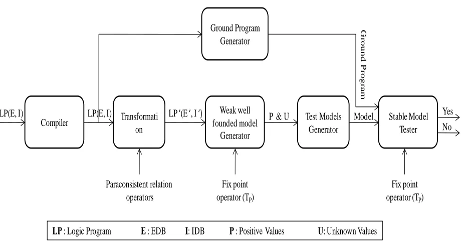
5.2 Overview of the Steps Involved
Figure 5.1 Block diagram for the proposed approach
The above figure shows the block diagram of various steps involved in the computation.
The process starts with compiling a logic program that performs the syntax and semantic checks
and produces a data structure called rules consisting of the logic program. These rules are then
transformed using the paraconsistent relation operators into another logic program consisting of
transformed rules. The transformed rules are then used to compute the weak well founded model
using the fix point operator. After the weak well founded model is computed the positive and the
unknown values are drawn from it and send to generate set of all possible models that are tested
for stability. The rules are also sent for ground program generation. The ground program and the
models for test are sent one by one to the stable model tester which tests each of them for
stability and returns a yes if model is stable and no otherwise. We also note the time taken to
Stable Model Tester Compiler Transformati
on
Weak well founded model
Generator
Test Models Generator Ground Program
Generator
LP(E, I) LP′(E′, I′) P & U Model
G
rou
nd
P
rog
ra
m
Paraconsistent relation operators
Fix point operator (TP)
Fix point operator (TP)
LP(E, I) Yes
No
complete the process of stable model computation. Next we describe each of the modules in
detail.
5.3 Modules
In this section we go over each of the modules in our described above. We start with the
compiler and the details about the Datalog language. Next we introduce two algorithms namely,
CONVERT and TRANSFORM in the transformation module. Then we go over model
generation for stability testing and ground program generation and finally the Stable model tester
is described.
5.3.1 Datalog Compiler
Datalog (one without function symbols) with negation, with a well defined declarative
semantics based on the work in logic programming has been widely accepted as standard
deductive database language [25, 26]. We use Datalog as our language and build a compiler so as
to do the syntax and semantic checks and create a data structure, for efficient storage of the logic
program. Some definitions related to Datalog.
Definition 15. Atomic formula:
a. p(x1, x2, …, xn) where p is a relation name (predicate name) and x1, x2, …, xn are variables
or constants. According to our assumption x1, x2, …, xn can only be variables in EDB.
b. x <op> y where x and y are either constants or variables and <op> is one of the
following six comparison operators: <, <=, >, >=, =, != . In our language we assume
Variables that appear only once in the rule can be replaced by anonymous variable (represented
by underscore). Every anonymous variable is different from all other variables.
Definition 16. Datalog rule:
p :- q1, q2, …, qn.
Where, p is an atomic formula and q1, q2, …, qn are either atomic formula or negated atomic
formula (i.e. atomic formula preceded by not). p is referred to as the head and q1, q2, …, qn are
referred to as subgoals of body.
Definition 17. Safe Datalog rule:
A Datalog rule p :- q1, q2, …, qn. is safe
a. If every variable that occurs in a negated subgoal also appears in a positive subgoal and
b. If variable that appears in the head of the rule also appears in the body of the rule.
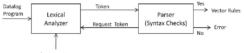
The compiler is build using the JFlex and JCup technologies that builds the lexer and parser. A
block diagram depicts the process. We input a logic program in the compiler and get a data
structure called rules as the output if there is no syntax or semantic errors.
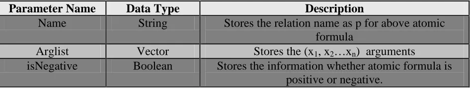
The data structure is build using two classes namely predicate and rule. The parameters and its
[image:42.612.68.541.627.716.2]types for the classes are shown below (using the definitions above):
Table 5.1 Predicate
Parameter Name Data Type Description
Name String Stores the relation name as p for above atomic formula
Arglist Vector Stores the (x1, x2…xn) arguments
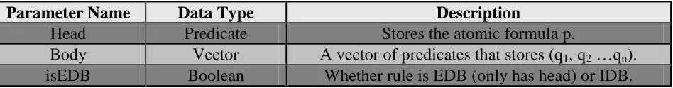
Table 5.2 Rule
Parameter Name Data Type Description
Head Predicate Stores the atomic formula p.
Body Vector A vector of predicates that stores (q1, q2 …qn).
isEDB Boolean Whether rule is EDB (only has head) or IDB. Finally, the data structure rules is a vector where each element is of type rule.
We also perform some semantic checks, which are as follows:
1. Arity Check: If an atomic formula appears more than once in the rules, then for its each
instance the argument list should be of the same size, i.e. if p(x1, x2…xn) and q(y1, y2,
…yn) are in logic program and if p = q, then n should be equal to m (n = m).
Example 5.3.1
(1) p(X, Y) :- r(X, Y, Z), s(X, Z).
(2) q(Z) :- r(X, Y), s(Z).
the above program has error as the relation named r has argument lists of size 2 in rule 1
and of size 3 in rule 2.
2. Safety Checks
a. Every variable that appears in negated subgoal should appear in the positive
subgoal. Suppose there is rule of the form:
p(X, Y) :- r(X, Y), not s(X, Z)
then the rule is not safe as the variable Z only appears in a negative subgoal and
not in a positive subgoal.
b. Every variable that appears in the head of the rule must appear in the body of the
rule. Suppose there is rule as follows:
is not safe as variable Y does not appear in the body of the rule.
Once we get an error free logic program we move to the next step that is transformation of the
logic program into a new logic program.
5.3.2 Transformation
We now present a transformation of a general deductive database P. In this method the
paraconsistent relations are the semantic objects associated with the predicate symbols in P. The method
involves two steps. The first step is to convert P into a set of paraconsistent relation definitions for
predicate symbols occurring in P taken from [21]. These definitions are of the form
p = Dp,
where, p is a predicate symbol of P, and Dp is an algebraic expression involving predicate
symbols of p and paraconsistent relation operators. The second step is to generate a new logic
program from the algebraic expression that can be used to compute the weak well founded
model.
Before describing the method to convert the given database P into set of definitions for
predicate symbol in P, let us look at an example. Suppose the following are the only clauses with
the predicate symbol p in their heads:
p(X) ← r(X, Y), ¬p(Y)
p(Y) ← s(Y, Z)
From these clauses the algebraic definition constructed for symbol p is the following:
Such a conversion exploits the close connection between attribute names in relation schemes and
variables in clauses, as pointed out in [25]. The expression thus constructed can be used to arrive
at a better approximation of paraconsistent relation p from some approximations of p, r and s.
We now give the algorithm to convert one clause into an expression.
The algorithm presented here is a modification of the original convert algorithm as our
deductive database does not involve any select conditions and the terms of IDB do not contain
constant values.
Algorithm 1 CONVERT
Input: A general deductive database clause l0 ← l1, l2, …, lm.
Let l0 be of the form p0(A01, …, A0k0), and each li, 1 ≤ i ≤ m, be either of the form pi(Ai, …, Aiki) or
of the form ¬pi(Ai, …, Aiki). For any i, 1 ≤ i ≤ m, let Vi be the set of all variables occurring in li.
Output: An algebraic expression involving paraconsistent relations.
Method: The expression is constructed using the following steps:
1. Let 𝑙 i be the atom pi(Bi1, …, Biki) and Fi be the conjunction of Ci1 ˄ Ci2 … ˄ Ciki. If li is a
positive literal, then let Qi, be the expression 𝜋 Vi(𝜎𝐹𝑖 𝑙 𝑖 )). Otherwise, let Qi be the
expression − 𝜋 Vi(𝜎𝐹𝑖 𝑙 𝑖 )).
As a syntactic optimization, if all conjuncts of Fi are true (i.e. all argument of li are distinct
variables), then both 𝜎 𝐹𝑖 and 𝜋 Vi are reduced to identity operations, and hence are dropped from
the expression. For example, if li = ¬p(X, Y), then Qi = − p(X, Y). As our language does not
2. Let E be the natural join (⋈) of Qi’s thus obtained, 1 ≤ i ≤ m. The output expression is
(𝜋 V(E))[B01, …, B0k0], where V is the set of variables occurring in 𝑙 0.
From the algebraic expressions obtained by algorithm CONVERT for all clauses in general deductive
database we construct another logic program using algorithm Transform.
Before going to transform we give an example from [13] of a deductive database and application of
convert algorithm on its clauses.
Example 5.3.2
This example represents a circuit consisting of an unusual sort of a logic gate, with one positive input X,
and one negative input Y, the its output is 1 or “true” if and only if X is 1 and Y is 0(“false”). There is an
EDB predicate g(X, Y, Z) that says there is a gate of this type with positive input X, negative input Y, and
output Z. We may think of inputs and outputs as being terminal or wire nets. There is also an EDB
predicate t0 that is true of those input terminals that are externally set to 1. Input terminals that are set to 0
do not appear in t0.
The IDB predicate is t. The intended significance of the positive ground atom t(a) being in the
model is that the circuit value of terminal a is 1. If ¬t(a) is in the model, then the value of terminal is 0.
What if the value that terminal a has ambiguous; either it depends on critical race in the circuit or
oscillates in normal circuit operation? Then, we expect t(a) to have a third, “unknown” value of three
valued logic. The following are the rules defining the operation of the gates:
t0(2).
g(5,1,3).
g(3,4,5).
t(Z) :- t0(Z) .
t(Z) :- g(X, Y, Z), t(X), not t(Y) .
The data in the EDB i.e. t0(2), g(5, 1, 3), g(1, 2, 4) and g(3, 4, 5) represents the circuit of Figure
[image:47.612.210.408.256.413.2]5.5.2 with only second input set to true.
Figure 5.2 Circuit for Example 5.5.2
We now apply Algorithm CONVERT on the two IDB clauses:
1. t(Z) :- t0(Z). The expression of this is t(Z) :- t0(Z).
2. t(Z) :- g(X, Y, Z), t(X), not t(Y). The positive literals g(X, Y, Z) and t(X) remain the same and the
literal not t(Y) becomes − t(Y). Then on the application of step 2 we get the following as the
algebraic expression:
t(Z) :- 𝜋 [Z](E)
When we get the algebraic expressions for all the clauses of IDB we move to the next
step. Here we introduce the algorithm TRANSFORM that takes these algebraic expressions as
input and returns a logic program as output. This logic program contains positive and negative
parts for all the different predicate symbols including the EDB relations. The transformation
converts the potentially harmful negation in the logic program into harmless negation. We also
create some new relations like the temporary and domain.
Algorithms 2 TRANSFORM
Input: EDB clauses and Algebraic expressions involving paraconsistent relations for IDB
clauses.
Output: A general logic program consisting of clauses of the form l0 ← l1, l2, …, lm.
Let l0 be of the form p0(A01, …, A0k0), and each li, 0 ≤ i ≤ m, be either of the form pi(Ai, …, Aiki) or
of the form ¬pi(Ai, …, Aiki).
Method: The logic program is constructed is using the following steps.
1. Transform the EDB clauses
a. Let a1,…, an be the constants present in EDB. Then, for each constant value aicreate
the following predicates with dom (domain) as the predicate symbol as follows
dom (a1).
:
b. Let l1,…,ln be the EDB predicates, where li is pi(B1,…,Bm), B1,..,Bm are constants, and
1 ≤ i ≤ n. Complete each EDB predicate pi as follows. Firstly, rename the existing
predicates and add it to the new logic program:
p1_plus(B1, ..., Bm).
:
pn_plus(B1,…, Bm).
For each unique predicate name pi in EDB add a rule as follows:
pi_minus(V1,…,Vn) :- dom(V1), dom(V2),…, dom(Vn), not pi_plus(V1,…, Vn).
where, V1,…,Vn are variables.
For example there are two EDB predicates p(1, 2) and p(2, 3) then we add the
following predicates, p_plus(1, 2), p_plus(2, 3) and a rule written below to the new logic
program.
p_minus(X, Y) :- dom(X), dom(Y), not p_plus(X, Y).
2. Renaming: If n IDB expressions have head with same predicate name p, and n > 1,
then, rename the clauses as p1, p2, …, pnin the algebraic expression. Let the argument
list be (V1, …, Vm) where V1,…, Vm are variables. Add the following positive predicates to
the logic program:
p_plus(V1,…,Vm) :- p1_plus(V1,…,Vm).
:
Add the following rule for the negative predicate.
p_minus(V1,…,Vm) :- p1_minus(V1,…,Vm), …., pn_minus(V1,…,Vm).
And, add the following rule for unknown values.
p_unknown(V1,…,Vm) :- dom(V1), …, dom(Vm), not p_plus(V1,…,Vm) , not
p_minus(V1,…,Vm).
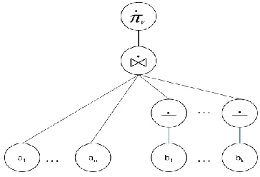
3. Construct paraconsistent trees for each IDB expression.
a. Let the IDB clause be l0 ← l1, …, ln, p1,…,pm where, l1, …, ln are positive
literals and p1, …, pm are negative literals. For this clause let the following be
the algebraic expression:
l0 :- (𝜋 V(E))[B01, …, B0k0]
where, V is the set of variables occurring in l0 and E is the natural join of l1, …, ln,
p1,…,pm.
Let l0 = p(B1, …, Bn), li = ai(C1,…, Cm) , where 1 ≤ I ≤ m and pj = ¬ bj(D1, …, Dk)
where 0 ≤ j ≤ k, and C1,…, Cm and D1,…, Dk are variables. So, the paraconsistent
[image:50.612.220.402.578.702.2]tree of the above expression would be depicted as follows:
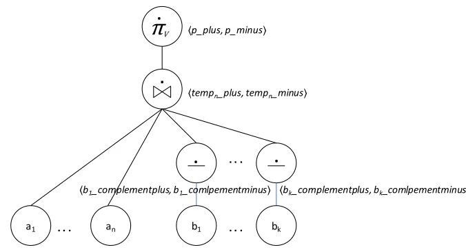
b. Naming the tree
i. Name the child node ai for 1 ≤ i ≤ n with its pair 〈ai_plus, ai_minus〉.
ii. Name the complement (− ) nodes with child node as bj as a pair
〈bk_complementplus, bk_complementminus〉, where 0 ≤ j ≤ k.
iii. If join (⋈ ) is an internal node name it tempn where n is the nth rule in IDB.
iv. Name the root node with the head predicate p as a pair 〈p_plus, p_minus〉.
[image:51.612.184.522.297.480.2]The named tree of figure 5.2.3 is as follows:
Figure 5.4 Named paraconsistent tree
4. Create rules for paraconsistent trees of all IDB expressions using the steps below.
Start writing rules bottom-up for all internal nodes.
a. If node type is complement (− ) and the child node is predicate c(B1, B2, …,
Bn).
c_complementplus(B1, B2, …, Bn) :- c_minus(B1, B2, …, Bn).
c_complementminus(B1, B2, …, Bn) :- c_plus(B1, B2, …, Bn). .
a1
π
V. . . . . .
. . .
an b1 bk
. . .
〈a1_plus, a1_minus〉 〈an_plus, an_minus〉 〈b1_plus, b1_minus〉 〈bk_plus, bk_minus〉
〈bk_complementplus, bk_comlpementminus〉 〈tempn_plus, tempn_minus〉
〈p_plus, p_minus〉
b. If node type is join (⋈ ) and it is the root node named 〈p_plus, p_minus〉, with
the child nodes named as 〈c1_plus, c1_minus〉,…,〈cn_plus, cn_minus〉 then
add the following rules:
p_plus(B1,…Bz) :- c1_plus(V1, …, Vm),…, cn_plus(T1,…Tk).
Also, add n rules where, n is the number of child nodes, and 1 ≤ i ≤ n as follows:
p_minus(B1,…Bz):- ci_minus(U1,…,Um).
if m < n that is if B1,…Bj = U1, …, Um andi ≤ j ≤z, then extend the rule by
adding dom predicates for Bj,…Bz to the above rule:
p_minus(B1,…Bn):- ci_minus(U1,…,Um), dom(Bj), …., dom(Bz).
c. If node type is join (⋈ ) and it is an internal node named tempn with child
nodes named as 〈c1_plus, c1_minus〉,…,〈cn_plus, cn_minus〉, then let the argument list of temp be V, where V is the set of all the variables occurring
the child nodes of tempn. And we add the rule as follows:
tempn_plus(V) :- c1_plus(V1, …, Vm),…, cn_plus(T1,…Tk).
Also, add n rules where, n is the number of child nodes, and 1 ≤ i ≤ n as follows:
tempn_minus(V) :- ci_minus(U1,…,Um), dom(B1), …., dom(Bz).
where B1,…, Bz are the set of variables not present in U1,.., Um.
d. If node type is projection (𝜋 V) named p, and V is the set projected variables, and
the child node is named tempn. In tempn , variables that do not appear in V are
anonymous and can be denoted by underscore.
(represent the projected variables in temp and rest of them with underscore)
We add three more rule for the negative predicate as follows:
tempn1(A1,…, An) :- dom(A1),…, dom(An).
tempn2(V) :- tempn1(A1,…,An), not tempn_minus(A1,…,An).
p_minus(V) :- dom(V1),..,dom(Vn), not tempn2(V).
Where, A1,…, An is the set of variables in child node tempn and V1,…, Vn are the
set of variables in V.
e. If the expression tree is a single child tree and it does not involve even
projection then for such tree we write the rules as follows. If root node is
named 〈p_plus, p_minus〉 and the child node is 〈c_plus, c_minus〉 then the
rules are:
p_plus(B1,…, Bn) :- c_plus(B1,…, Bn).
p_minus(B1,…, Bn) :- c_minus(B1,…, Bn).
5. For each unique IDB predicate p, except for those created in Step 2, add the following
rule for unknown values:
p_unknown(B1...Bn) :- dom(B1),…,dom(Bn), not p_plus(B1,…, Bn), not p_minus(B1,…, Bn).
The TRANSFORM algorithm removes the „harmful negation‟ or we can say the unsafe
negation from the original program because with each negative predicate it introduces the dom
predicates, which are joined with the negative predicate, that limits the domain to all constant
value present in the Herbrand base. This could otherwise cause safety issue as to negation of a