Quantification of surface water volume changes in the Mackenzie Delta using satellite multi mission data

https://doi.org/10.5194/hess-22-1543-2018 © Author(s) 2018. This work is distributed under the Creative Commons Attribution 3.0 License.

Quantification of surface water volume changes in the Mackenzie

Delta using satellite multi-mission data

Cassandra Normandin1, Frédéric Frappart2,3, Bertrand Lubac1, Simon Bélanger4, Vincent Marieu1, Fabien Blarel3, Arthur Robinet1, and Léa Guiastrennec-Faugas1

1_{EPOC, UMR 5805, Université de Bordeaux, Allée Geoffroy Saint-Hilaire, 33615 Pessac, France} 2_{GET-GRGS, UMR 5563, CNRS/IRD/UPS, Observatoire Midi-Pyrénées, 31400 Toulouse, France} 3_{LEGOS-GRGS, UMR 5566, CNRS/IRD/UPS, Observatoire Midi-Pyrénées, 31400 Toulouse, France} 4_{Dép. Biologie, Chimie et Géographie, groupe BOREAS and Québec-Océan, Université du}

Québec à Rimouski, 300 allée des ursulines, Rimouski, Qc, G5L 3A1, Canada Correspondence:Cassandra Normandin ([email protected]) Received: 22 March 2017 – Discussion started: 29 May 2017

Revised: 5 December 2017 – Accepted: 11 January 2018 – Published: 28 February 2018

Abstract. Quantification of surface water storage in exten-sive floodplains and their dynamics are crucial for a bet-ter understanding of global hydrological and biogeochemi-cal cycles. In this study, we present estimates of both surface water extent and storage combining multi-mission remotely sensed observations and their temporal evolution over more than 15 years in the Mackenzie Delta. The Mackenzie Delta is located in the northwest of Canada and is the second largest delta in the Arctic Ocean. The delta is frozen from October to May and the recurrent ice break-up provokes an increase in the river’s flows. Thus, this phenomenon causes intensive floods along the delta every year, with dramatic environmen-tal impacts. In this study, the dynamics of surface water ex-tent and volume are analysed from 2000 to 2015 by com-bining multi-satellite information from MODIS multispec-tral images at 500 m spatial resolution and river stages de-rived from ERS-2 (1995–2003), ENVISAT (2002–2010) and SARAL (since 2013) altimetry data. The surface water ex-tent (permanent water and flooded area) peaked in June with an area of 9600 km2 (±200 km2) on average, representing approximately 70 % of the delta’s total surface. Altimetry-based water levels exhibit annual amplitudes ranging from 4 m in the downstream part to more than 10 m in the up-stream part of the Mackenzie Delta. A high overall corre-lation between the satellite-derived and in situ water heights (R> 0.84) is found for the three altimetry missions. Finally, using altimetry-based water levels and MODIS-derived sur-face water extents, maps of interpolated water heights over

the surface water extents are produced. Results indicate a high variability of the water height magnitude that can reach 10 m compared to the lowest water height in the upstream part of the delta during the flood peak in June. Furthermore, the total surface water volume is estimated and shows an annual variation of approximately 8.5 km3during the whole study period, with a maximum of 14.4 km3observed in 2006. The good agreement between the total surface water vol-ume retrievals and in situ river discharges (R=0.66) allows for validation of this innovative multi-mission approach and highlights the high potential to study the surface water extent dynamics.

1 Introduction

the surface water reservoir in circumpolar areas is crucial for a better understanding of their role in flood hazard, carbon production, greenhouse gases emission, sediment transport, exchange of nutrients and land–atmosphere interactions.

Mapping surface water extent on the scale of the Macken-zie Delta is an important issue. However, it is nearly impos-sible to provide long-term monitoring with traditional meth-ods using in situ measurements in such a large and heteroge-neous environment. Satellite remote sensing method offers a unique opportunity for the continuous observation of wet-lands and floodplains. Remote sensing has been proven to have strong potential to detect and monitor floods during the last 2 decades (Alsdorf et al., 2007; Smith, 1997). Typically, two kinds of sensor are used to map flooded areas at high and moderate resolutions: passive multispectral imagery and ac-tive synthetic aperture radar (SAR). The spectral signature of the surface reflectance is used to discriminate between water and land (Rees, 2013). The SAR images provide valuable in-formation on the nature of the observed surface through the backscattering coefficient (Ulaby et al., 1981).

If space missions of radar altimetry were mainly dedicated to estimate ocean surface topography (Fu and Cazenave, 2001), it is now commonly used for monitoring inland wa-ter levels (Birkett, 1995; Cazenave et al., 1997; Frappart et al., 2006a, 2015b; Santos da Silva et al., 2010; Crétaux et al., 2011a, 2017). Several studies have shown the possibility to measure water levels variations in lakes, rivers and flood-ing plains (Frappart et al., 2006b, 2015a; Santos da Silva et al., 2010). In the present study, satellite multispectral im-agery and altimetry are used in synergy to quantify surface water extents and the surface water volumes of the Macken-zie Delta and analyse their temporal variations. In the past, this approach has been applied in tropical (e.g. the Amazon, Frappart et al., 2012; Mekong, Frappart et al., 2006b) and peri-Arctic (e.g. the Lower Ob’ basin, Frappart et al., 2010) major river basins, allowing direct observations of the spatio-temporal dynamics of surface water storage. Several limita-tions prevent their use over estuaries and deltas. The first is the too-coarse spatial resolution of the datasets used for re-trieving the flood extent that ranges from 1 km with SPOT-VGT images used in the lower Mekong Basin to∼0.25◦with the Global Inundation Extent from Multi-Satellite (GIEMS, Papa et al., 2010) dataset for the Lower Ob’ and the Amazon basins. The second is inherent to the datasets used in these studies. For the Mekong Basin, due to the limited number of spectral bands present in the VGT sensor, a mere threshold on the normalized difference vegetation index (NDVI) was applied. For the Amazon and the Lower Ob’, as the GIEMS dataset is using surface temperatures from the Special Sen-sor Microwave Imager (SSM/I), no valid data are available at less than 50 km from the coast. The originality and novelty of the study stem from the use of multi-space mission data at better spatial, temporal and spectral resolutions than the pre-vious studies to monitor surface water storage changes in a deltaic environment over a 15-year time period.

Earlier studies pointed out (i) the lack of continuous in-formation in the Mackenzie delta to study the spatial distri-bution of water levels during the flood events and to anal-yse the relationship between flood severity and the timing and duration of break-up in the delta (Goulding et al., 2009b; Beltaos et al., 2012) and (ii) the importance of the tributaries to the Mackenzie River (i.e. Peel and Arctic Red rivers) on break-up and ice-jam flooding in the delta (Goulding et al., 2009a). As the goal of this study is to characterize the spatio-temporal surface and storage dynamics of surface water in the Mackenzie delta, Northwest Territories of Canada, in re-sponse to spring ice break-up and snow melt, over the period 2000–2015, it will provide important new information for a better understanding of the hydro-climatology of the region.

2 Study region

The Mackenzie Delta, a floodplain system, is located in the northern part of Canada (Fig. 1a) and covers an area of 13 135 km2 (Emmerton et al., 2008), making it the second biggest delta of Arctic with a length of 200 km and a width of 80 km (Emmerton et al., 2008). It is mainly drained by the Mackenzie River (90 % of the delta’s water supply) and Peel River (8 % of the delta’s water supply, Emmerton et al., 2007). The Mackenzie Delta channels have very mild slopes (−0.02 m km−1; Hill et al., 2001), and are ice-covered during 7–8 months per year (Emmerton et al., 2007).

The Mackenzie River begins in the Great Slave Lake and then, flows through the Northwest Territories before reaching the Beaufort Sea. It has a strong seasonality in term of dis-charge due to spring ice break-up and snowmelt, from about 5000 m3s−1_{in winter up to 40 000 m}3_s−1_{in June during the}

ice break-up for wet years (Fig. 1b, Macdonald and Yu, 2006; Goulding et al., 2009a, b; Beltaos et al., 2012). The Stamukhi (ground accumulation of sea ice) is responsible for recurrent floods in the Mackenzie Delta. At the flood peak, 95 % of the delta surface is likely to be covered with water (Macdonald and Yu, 2006). Water level peaks are mainly controlled by ice break-up effects and secondarily by the amount of wa-ter contained in snowpack (Lesack and Marsh, 2010). This is one of the most important annual hydrologic events in cold regions (Muhammad et al., 2016).

Figure 1. (a)Location of the Mackenzie Delta at the mouth of the Mackenzie River in the Northwest Territories of Canada.(b) River discharges of the Mackenzie River at 10LC014 station from 2000 to 2015 (133◦W, 67◦N), 30 km upstream the Mackenzie Delta.

3 Datasets

3.1 Multispectral imagery 3.1.1 MODIS

The Moderate Resolution Imaging Sensor (MODIS) is a spectroradiometer, part of the payload of the Aqua (since 2002) and Terra (since 1999) satellites. The MODIS sen-sor measures radiances in 36 spectral bands. In this study, the MOD09A1 product (8-day binned level 3, version 6) de-rived from Terra satellite surface reflectance measurements were downloaded from the United States Geological Sur-vey (USGS) EarthExplorer website (https://ladsweb.modaps. eosdis.nasa.gov/). It consists of gridded, atmospherically cor-rected surface reflectance acquired in seven bands from visi-ble to shortwave infrared (SWIR) (2155 nm) at a 500 m spa-tial resolution. This product is obtained by combining for each wavelength the best surface reflectance data of every pixel acquired during an 8-day period. Each MODIS tile covers an area of 1200 km by 1200 km. Two tiles (h12v02 and h13v02) are used to cover the whole study area. In this study, 223 composites, acquired during the ice-free period from June to September over the 2000–2015 time span, are used.

3.1.2 OLI

The Landsat-8 satellite is composed of two Earth-observing sensors, the Operational Land Imager (OLI) and Thermal In-fraRed Sensor (TIRS). This satellite was launched in Febru-ary 2013 and orbits at an altitude of 705 km. The swath is 185 km and the whole Earth surface is covered every 16 days. The OLI–TIRS sensors measure in 11 spectral bands in the visible (450–680 nm), near-infrared (845–885 nm) and shortwave infrared (1560–2300 nm) portions of the electro-magnetic spectrum. In this study, the Landsat-8 OLI surface reflectance products were downloaded from the Landsat-8 USGS portal (http://earthexplorer.usgs.gov/). The multispec-tral spatial resolutions are 30 and 15 m for panchromatic bands. Two images are necessary to cover the Mackenzie Delta.

res-olution. However, available high-quality OLI data have been used to compare and validate MODIS water surface areas. 3.2 Radar altimetry data

3.2.1 ERS-2

The ERS-2 satellite (European Remote Sensing) was launched in 1995 by the European Space Agency (ESA). Its payload is composed of several sensors, including a radar al-timeter (RA), operating at the Ku band (13.8 GHz). It was

orbiting sun-synchronously at an altitude of 790 km with an inclination of 98.54◦ with a 35-day repeat cycle. This orbit was ERS-1’s orbit with a ground-track spacing about 85 km at the Equator. ERS-2 provides observations of the topog-raphy of the Earth from 82.4◦_{latitude north to 82.4}◦_latitude

south. ERS-2 data are disposable from 17 May 1995 to 9 Au-gust 2010 but after 22 June 2003, the coverage is limited. 3.2.2 ENVISAT

Envisat mission was launched on 1 March 2002 by ESA. This satellite carried 10 different instruments including the advanced radar altimeter (RA-2). It was based on the her-itage of ERS-1 and 2 satellites. RA-2 was a nadir-looking pulse-limited radar altimeter operating at two frequencies at Ku (13.575 GHz) and S (3.2 GHz) bands. Its goal was to

collect radar altimetry over ocean, land and ice caps (Zelli, 1999). Envisat remained on its nominal orbit until October 2010 but RA-2 stopped operating correctly at the S band in January 2008. Its initial orbital characteristics are the same as for ERS-2.

3.2.3 SARAL

SARAL mission was launched on 25 February 2013 by a partnership between CNES (Centre National d’Etudes Spa-tiales) and ISRO (Indian Space Research Organization). Its payload comprised the AltiKa radar altimeter and bi-frequency radiometer, and a triple system for precise or-bit determination: the real-time tracking system DIODE of the DORIS instrument, a laser retroflector array (LRA), and the Advance Research and Global Observation Satellite (ARGOS-3). AltiKa is the first radar altimeter to operate at the Kaband (35.75 GHz). It is a solid-state mono-frequency

altimeter that provides precise range estimates (Verron et al., 2015). SARAL orbit was earlier utilized by ERS-1 & 2 and ENVSAT missions with a track spacing of 85 km at the Equa-tor (Verron et al., 2015). It has been put on a drifting orbit since 4 July 2016.

Altimetry data used here are contained in the Interim Geo-physical Data Records (GDRs) and are the following:

– cycle 001 (17 May 1995) to cycle 085 (7 August 2003) for ERS-2 from the reprocessing of the ERS-2 mission raw waveform performed at Centre de Topographie de

l’Océan et de l’Hydrosphère (CTOH) (Frappart et al., 2016)

– GDR v2.1 for ENVISAT from cycle 006 (14 May 2002) to cycle 094 (21 October 2010)

– GDR E for SARAL from cycle 001 (15 March 2015) to cycle 027 (14 October 2015).

These data were made available by CTOH (http://ctoh.legos. obs-mip.fr/). Data were acquired along the altimeter track at 18, 20 and 40 Hz for ENVISAT, ERS−2 and SARAL respec-tively (high-frequency mode commonly used over land and coastal areas where the surface properties are changing more rapidly than over the open ocean). They consist of the satel-lite locations and acquisition times and all the parameters necessary to compute the altimeter heights (see Sect. 4.3). 3.3 In situ water levels and discharges

The altimetry-based water level time series derived from radar altimetry were compared to gauge records from in situ stations for validation purpose. Data from 10 gauge sta-tions were found in close vicinity to altimetry virtual stasta-tions (VSs; at a distance of less than 20 km along the streams). Vir-tual stations are built at intersections between an orbit ground rack and a water body (lake, river and floodplain) (Crétaux et al., 2017). Besides, surface water storage variations were compared to the river flow entering the delta, summing the records from three gauge stations located in upstream part of the delta. Daily data of water level and discharge were downloaded for free from the Canadian government website (http://wateroffice.ec.gc.ca).

4 Methods

4.1 Quantification of surface water extent

depen-dent on the Earth surface nature, in particular water versus soil–vegetation surfaces, their complement was used to de-fine LSWI. For instance, the surface reflectance presents low values (a few percentage points) over non-turbid water bod-ies and high values (a few tens of percentage points) over vegetation feature in the NIR spectral bands. The spectral response in the SWIR is mainly dominated by strong water absorption bands, which is directly sensitive to moisture con-tent in the soil and the vegetation. For water surface area, the signal in the SWIR is assumed to be zero even in turbid wa-ters (Wang and Shi, 2005). Thus, LSWI is expected to get values close to 1 for water surface areas and lower values for non-water surface areas.

The two indices, used in this approach, are defined as fol-lows (Huete et al., 1997; Xiao et al., 2005):

EVI=a× ρNIR−ρred

ρNIR+b×ρred−c×ρblue+d

, (1)

LSWI=ρNIR−ρSWIR ρNIR+ρSWIR

, (2)

where for MODIS, ρblue is the surface reflectance value in

the blue (459–479 nm, band 3),ρredis the surface reflectance

value in the red (621–670 nm, band 1), ρNIR is the

sur-face reflectance value in the NIR (841–875 nm, band 2), and ρSWIRis the surface reflectance in the SWIR (1628–1652 nm,

band 6). For OLI, ρblue, ρred,ρNIR, andρSWIR are

associ-ated with channel 2 (452–512 nm), channel 4 (636–673 nm), channel 5 (851–879 nm), and channel 6 (1570–1650 nm), re-spectively. The constantsa, b, candd are equal to 2.5, 6, 7.5 and 1, respectively, for both MODIS and OLI (USGS, prod-uct guide).

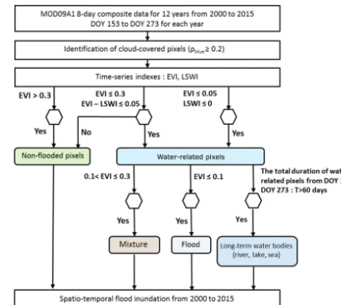
To process multispectral images, the first step consists of removing the cloud-contaminated pixels by applying a cloud masking based on a threshold of the surface reflectance in the blue band (ρblue≥0.2). Then, spectral indices are computed.

Note that, contrary to Sakamoto et al. (2007), no smooth-ing was applied on spectral index time series. In a second step, the identification of the status of each pixel is performed by applying thresholds on EVI, LSWI and their differences (Fig. 2), which reduce the noise component. Thresholds de-termined by Sakamoto et al. (2007) were validated for our study site using OLI images acquired on 1 July and 2 Au-gust 2013 and compared to MODIS (Fig. S1 in the Supple-ment). Histograms show a similar bi-modal distribution for both EVI, LSWI and EVI-LSWI between MODIS and OLI 500 m (Figs. S1 and S2). For EVI, pixels with a value lower than 0.1 are clearly associated with water land surfaces, while pixels with a value higher than 0.3 are associated with soil and vegetation features. Other pixels, with an EVI value be-tween 0.1 and 0.3, are identified as mixed surface types. For LSWI, pixels with a value higher than 0.5 are clearly associ-ated with water land surfaces, while pixels with a value lower than 0.3 are associated with vegetation features or soil land surfaces when LSWI values are negative. Other pixels, with an LSWI value between 0.3 and 0.5, are identified as mixed

Figure 2.Flow chart of the method (adapted from Sakamoto et al., 2007) used to classify each pixel of the multispectral images ac-quired over the Mackenzie Delta in four categories (non-flooded, mixed, flooded and permanent water bodies) for each year from 2000 to 2015 using MODIS 8-day composite data from the day of the year (DOY) 169 to 257.

surface types. Contrary to what was found by Sakamoto et al. (2007) in the Mekong Basin, no negative values of LSWI were observed over our study area. This threshold was not applied in this study. For EVI–LSWI, pixels with a value lower than−0.05 represent water land surface and values be-tween−0.05 and 0.1 are associated with mixed pixels. Other pixels, with values higher than 0.1 are represented vegetation features or soil land surfaces (Fig. S2). Each pixel was then classified in two main categories: non-flooded (EVI > 0.3 or EVI≤0.3 but EVI−LSWI > 0.05) and water-influenced (EVI≤0.3 and EVI−LSWI≤0.05 or EVI≤0.05) (Fig. 2). The second category was divided into three sub-classes: mixed pixels (0.1 < EVI≤0.3), flooded pixels (EVI≤0.1) and permanent water bodies (e.g. lake, river and sea), the latter denoting when the total duration of a pixel classified as flooded is longer than 70 days out of 105 days for the study period. This annual duration for our study corresponds roughly to two-thirds of the study period, as proposed by Sakamoto et al. (2007). The spatio-temporal variations of floods have been characterized for the months between June and September over the 2000–2015 period.

4.2 Validation of MODIS retrievals using OLI

Evaluation of the performance of the water surface area de-tection from MODIS is based on the comparison between land surface water estimated from MODIS at a 500 m resolu-tion, OLI at a 30 m resoluresolu-tion, and OLI re-sampled at 500 m resolution. For validation purposes, MODIS and OLI images are selected when (1) the time difference between the acqui-sitions of two satellite images is lower than 3 days and (2) the presence of cloud over the area is lower than 5 %. Following these criteria, only two cloud-free OLI composites were se-lected between 1 July and 2 August 2013.

4.3 Satellite-derived water level time series in the Mackenzie Delta

The concept of radar altimetry is explained below. The radar emits an electromagnetic (EM) wave towards the surface and measures the round-trip time (1t) of the EM wave. Taking into account propagation corrections caused by delays due to the interactions of electromagnetic waves in the atmosphere, and geophysical corrections, the height of the reflecting sur-face (h) with reference to an ellipsoid can be estimated as follows (Crétaux et al., 2017):

h=H−(R+X1Rpropagation+1Rgeophysical), (3)

whereHis the satellite centre of mass height above the ellip-soid,Ris the nadir altimeter range from the satellite centre of mass to the surface (taking into account instrument cor-rections;R=c1t /2, wherecis the light velocity in the vac-uum), andP_1R

propagationis the sum of the geophysical and

environmental corrections applied to the range. X

1Rpropagation=1Rion+1Rdry+1Rwet, (4)

where1Rionis the atmospheric refraction range delay due to

the free electron content associated with the dielectric prop-erties of the ionosphere,1Rdryis the atmospheric refraction

range delay due to the dry gas component of the troposphere, and1Rwet is the atmospheric refraction range delay due to

the water vapour and the cloud liquid water content of the troposphere.

X

1Rgeophysical=1Rsolid Earth+1Rpole, (5)

where1Rsolid Earthand1R pole are the corrections

respec-tively accounting for crustal vertical motions due to the solid Earth and pole tides. The propagation corrections applied to the range are derived from model outputs: the global ionospheric maps (GIMs) and Era-Interim datasets from the European Centre for Medium-Range Weather Forecasts (ECMWF) for the ionosphere and the dry and wet tropo-sphere range delays respectively. The changes in the altime-ter heighthover the hydrological cycles are related to vari-ations in water level. Here, the Multi-mission Altimetry Pro-cessing Software (MAPS) was used to precisely select valid

altimetry data at every virtual station location (see Sect. 3.3) series in the Mackenzie Delta. Data processing consisted of four steps (Frappart et al., 2015b):

– the rough delineation of the river–lake cross sections with overlaying altimeter tracks using Google Earth (distances of±5 km from the river banks are generally considered);

– the loading of the altimetry over the study area and the computation of the altimeter heights from the raw data contained in the GDRs;

– the selection of valid altimetry data through a refined process that consists of eliminating outliers and mea-surements over non-water surface areas based on visual inspection (the shape of the altimeter along-track pro-files permit identification of the river that is generally materialized as a shape of “V” or “U”, with the lower elevations corresponding to the water surface area; see Santos da Silva et al., 2010 and Baup et al., 2014 for more details);

– the computation of the time series of water level. 4.4 Surface water volume storage

The approach used to estimate the anomalies of surface ter volume is based on the combination of the surface wa-ter extent derived from MODIS images with altimetry-based water levels estimated at virtual stations distributed all over the delta (Fig. 5). Surface water level maps were computed from the interpolation of water levels over the water surface areas using an inverse-distance weighting spatial interpola-tion technique following Frappart et al. (2012). Hence, water level maps were produced every 8 days from 2000 to 2015. For each water pixel, the minimal height of water during 2000–2015 is estimated. As ERS-2, ENVISAT and SARAL had a repeat cycle of 35 days, water levels are linearly inter-polated every 8 days to be combined with the MODIS com-posite images.

Surface water volume time series are estimated over the Mackenzie Delta following Frappart et al. (2012):

V =X j S

[h(λj, ϕj)−hmin(λj, ϕj)] ·δj·1S, (6)

whereV is the anomaly of surface water volume (km3), S is the surface of the Mackenzie Delta (km2),h(λj,ϕj) the water level,hmin (λj, ϕj) the minimal water level for the

pixel of coordinates (λj, ϕj)inside the Mackenzie Delta,δj

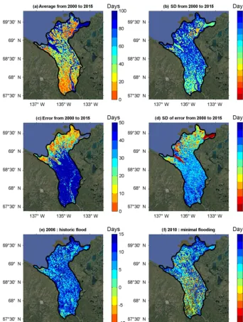
Figure 3.Maps of surface water extent duration for(a)annual average from 2000 to 2015,(b)annual standard deviation from 2000 to 2015,(c)error average from 2000 to 2015,(d)standard deviation from 2000 to 2015, difference between annual average water surface area duration from 2000 to 2015 and water surface area duration during(e)2006, the period associated with the highest flood event, and(f)2010, the period associated with the lowest flood event recorded over the period.

5 Results

5.1 MODIS-based land water extent and their validation

Following the method of Sakamoto et al. (2007), all pix-els of 8-day image have been classified into four groups: class 0 corresponding to vegetation, class 1 to permanent wa-ter, class 2 to inundation, and class 3 to a mixture of land and water. A map of annual average of water surface area, com-posed of inundated and permanent water bodies (classes 1

surrounding permanent water bodies. Other areas of the delta are annually inundated up to 30 days (Fig. 3a). The map of standard deviation of the annual flood duration shows ranges from a few days over the areas affected by floods during a short time span to 15 days close to permanent water bodies (Fig. 3b).

Maps of errors made on water surface area duration with associated standard deviation are shown in Fig. 3c and d over 2000–2015. Mixed pixels have been used to calculate the er-ror for each pixel on water surface area duration, correspond-ing to the class 3 “mixed” of Sakamoto et al. (2007) classi-fication. Standard deviation is presented in Fig. 3d. Maximal error and standard deviation is obtained for pixels of poten-tial flooding area in the delta. If short differences – lower than 20±12 days – can be observed in the downstream part of the delta (over 69◦N), longer differences (30 to 50±15 to 20 days) are present in the upstream part. They can be at-tributed to the presence of small permanent lakes in this area. Important inter-annual differences can be observed between wetter (Fig. 3e) and dryer (Fig. 3f) years.

Surface water extent (the sum of permanent bodies and in-undated areas) were also estimated by applying the approach described in Sect. 3.1 for OLI images at 30 m of spatial res-olution, and resampled at 500 m of spatial resolution. They were compared to MODIS-based surface water extent for the closest date (Table 1). Figure S3a, b and c present the maps of the surface water extent determined using MODIS, OLI 500 m and OLI 30 m respectively, acquired in July 2013. Medium and large-scale (with a minimal size of 300 m) land water features are well detected, as displayed in the enlarged part of the images. Figure S3c presents an enlarged image of surface water extent using OLI 30 m with permanent and in-undated bodies. Surface water extent from OLI 500 m and MODIS are similar for both dates, with differences lower than 20 % (Table 1). For example in July 2013, water sur-face area is about 4499 km2 for OLI 500 and 3798 km2for MODIS (Table 1). Percentages of common detection of sur-face water were estimated for the pixels detected as water surface area in the pair of satellite images. These percentages are 73 and 74 % for July and August 2013, respectively. Ar-eas detected as water by both sensors correspond to the main channels and connected floodplains. Differences appear on the boundaries of areas commonly detected as inundated and on small scales and can be attributed to the difference of ac-quisition dates between MODIS and OLI (Fig. S4). These results highlight the robustness of the method of Sakamoto et al. (2007) for accurate water surface area retrievals. These surface water extents have been compared with surface water extents (channels and wetlands) determined by Emmerton et al. (2007) in Table 1. For MODIS, differences are lower than 15 % and for OLI 500 differences are about 25 % (Table 1).

However, the comparison between surface water extent es-timated from OLI 30 m and MODIS 500 m shows impor-tant differences. In July 2013, surface water extent is about 3798 km2from MODIS and 7685 km2from OLI 30. The

sur-face extents are higher for OLI 30 by a factor of 2 (Table 1). According to Emmerton et al. (2007), the Mackenzie Delta is composed of 49 000 lakes with a mean area of 0.0068 km2 and 40 % of the total number of lakes have an area inferior to 0.25 km2. The pixel sizes of OLI 30 m and MODIS 500 m are approximately 0.0009 and 0.25 km2, respectively. Thus, the high difference between the water surface areas detected using OLI 30 m and MODIS is probably associated with a spatial sample bias. Small-scale water features detected from OLI cannot be detected from MODIS due to a lower spatial resolution.

Surface water extents determined using OLI 30 have been compared to Emmerton et al. (2007) surface water extents (including channels, wetlands and lakes). Emmer-ton et al. (2007) classified the Mackenzie Delta habitat in lakes, channels, wetlands and dry floodplains using informa-tion from topographic maps derived from aerial photographs taken during the 1950s for low-water periods. Differences between surface water extent of OLI 30 and Emmerton et al. (2007) are lower than 15 % (Table 1).

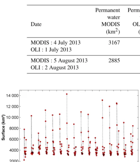
In order to investigate the assumption of spatial sample bias associated with MODIS 500 m, a satellite validation of surface water extent is performed (Table 2). Permanent wa-ter and inundated surfaces have been calculated for MODIS, OLI 500 and OLI 30. For OLI 30 and OLI 500, pixels identi-fied as surface water for the two dates are considered as per-manent waters (Table 2). In July 2013, inundated surfaces are nearly equal, about 577 km2 for MODIS, 690 km2for OLI 500 and 627 km2for OLI 30 (Table 2). In August, inundated surfaces are equal to 250 km2and are 2.5 times more impor-tant than OLI 30 (98 km2), if we consider OLI 30 as truth.

Table 1.Validation of surface water extents (km2) determined using OLI 30 m, OLI 500 m, and MODIS 500 m images with the results of Emmerton et al. (2007).

MODIS: 4 July 2013 MODIS: 5 August 2013 OLI: 1 July 2013 OLI: 2 August 2013

MODIS 500 m 3798 3298

OLI 500 m 4499 3859

Emmerton et al. (2007) (channels+wetlands, km2)

3358 3358

Difference between MODIS 500 and Emmerton et al. (2007)

440 km2(13 %) 60 km2(2 %)

Difference between OLI 500 and Emmerton et al. (2007)

1141 (34 %) 500 (15 %)

OLI 30 m 7685 7156

Emmerton et al. (2007)

(channels+lakes+wetlands, km2)

6689 6689

Difference between OLI 30 and Emmerton et al. (2007)

996 km2(13 %) 467 km2(7 %)

Table 2.Satellite validation of surface water extent using OLI 30, OLI 500 and MODIS 500 m.

Permanent Permanent Permanent Inundated Inundated Inundated

water water water surfaces surfaces surfaces

Date MODIS OLI 500 OLI 30 MODIS OLI 500 OLI 30

(km2) (km2) (km2) (km2) (km2) (km2)

MODIS : 4 July 2013 3167 3809 7058 577 690 627

OLI : 1 July 2013

MODIS : 5 August 2013 2885 3809 7058 250 50 98

OLI : 2 August 2013

Figure 4.Time series of surface water extent from 2000 to 2015, between June and September, derived from the MODIS images.

24 altimetry virtual stations were built at the cross section of an altimetry track with a water body for these three mis-sions respectively (see Fig. 5 for their locations). A water level temporal series is obtained for each virtual station.

The quality of altimetry-based water levels was evaluated using in situ gauge records. Only 6 virtual stations are lo-cated near in situ stations (with a distance lower than 20 km) for ERS-2 data, with 10 for ENVISAT and 8 for SARAL data. Characteristics of these virtual stations are given in Ta-ble 3. For ERS-2 and SARAL comparisons, the correlationr is low at the station 0114-c, i.e.−0.38 and 0.15 respectively (Table 3).

For ERS-2, quite high correlation coefficients are ob-tained for four virtual stations out of six, withr≥0.69 and RMS≤1 m (Table 3). For the two other stations, no correla-tion is observed (−0.38 and 0.08 for 2-0114c and ERS-2-0200-d respectively with a RMS≥1 m) (Table 3).

Table 3.Statistic parameters obtained between altimetry-based water levels from altimetry multi-mission and in situ water levels.

Virtual station (SV)

In situ station Altimetry mission Distance (km) River width at VS (m)

N r RMS

(m)

R2 Bias

(m)

Bias ICESat (m)

0439-a 10MC008 ERS-2

ENVISAT SARAL

11.44 1950 5

24 8 0.76 0.89 0.96 0.5 0.5 0.35 0.58 0.81 0.93 0.55 0.15 −0.95 1.36 0.65 −0.15

0983-c 10MC003 ERS-2

ENVISAT SARAL

3.1 360 20

26 6 0.69 0.66 0.9 0.7 0.89 0.4 0.47 0.44 0.8 – – – – – –

0114-c 10MC022 ERS-2

ENVISAT SARAL

1.9 430 14

23 7 −0.38 0.8 0.14 2.82 1.17 0.73 0.14 0.64 0.02 – – – – – –

0200-d 10MC023 ERS-2

ENVISAT SARAL

4.11 630 17

22 6 0.08 0.87 0.76 4.3 0.33 0.3 0 0.75 0.57 – – – – – –

0744-a 10MC010 ERS-2

ENVISAT SARAL

5.16 850 5

24 2 0.88 0.93 0.99 0.1 0.15 0.15 0.77 0.87 0.99 – – – −1.28 −1.17 −2.19

0439-d 10LC015 ERS-2

ENVISAT SARAL

7.2 380 20

28 5 0.92 0.65 0.95 0.83 1.75 1.3 0.86 0.43 0.9 – – – – – –

0525-a 10MC002 ENV 16.31 500 29 0.77 1.45 0.6 – –

0028-a 10LC014 ENV 16.05 1360 17 0.83 1.84 0.7 – 2.35

Figure 5.Locations of virtual stations (VSs) in the Mackenzie Delta for ERS-2 (yellow dots), Envisat (green dots) and SARAL (purple dots) altimetry missions. Altimetry tracks appear in grey. In situ stations are represented using red triangles.

section was only 150 m wide (Table 3). This station is also lo-cated near the city of Inuvik. The presence of the town in the altimeter footprint could exert a strong impact on the radar echo and explain this low correlation.

For SARAL, five out of six virtual stations have a good correlationr coefficient higher than 0.76 with a low RMS (Table 3) due to its narrower footprint with an increase in the along-track sampling.

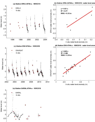
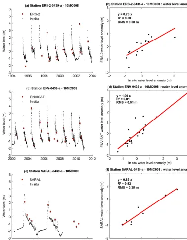
Comparisons between water levels derived from altime-try and in situ are shown for two stations for ERS-2 (called ERS-2-0744-a and ERS-2-0439-a; Figs. 6a and 7a), three for ENVISAT (ENV-0744-a, ENV-0439-a and ENV-0028-a; in Figs. 6b, 7b and 8) and two for SARAL (SARAL-0744-a and SARAL-0439-a; Figs. 6c and 7c). Virtual station 0744-a is loc0744-ated in the downstre0744-am p0744-art of the delt0744-a, 0439-0744-a in the centre and 0028-a in the upstream part (Fig. 5). For each station, water levels obtained by altimetry and water levels obtained by in situ gauges are superposed (Figs. 6, 7 and 8). Then, water level anomalies, which are computed as the av-erage water level minus the water level, have been calculated for altimetry and in situ data.

Figure 6.Altimetry-based water levels from 1995 to 2015 compared with in situ water levels for the station 0744-a, located in the downstream part in the Mackenzie Delta, using(a)the ERS-2 mission and(b)a water level anomaly with statistic parameters,(c)the ENVISAT mission and(d)a water level anomaly with statistic parameters, and(e)using SARAL mission.

data of the station 10MC010 for each mission ERS-2, EN-VISAT and SARAL (Fig. 6). In situ data are not continuous since the river is frozen from October to April. With regard to altimetry, data have been acquired throughout the year, but during frozen periods water levels are unrealistic due to the presence of river ice. Thus, the processing is done only from the beginning of June to the end of September for multispec-tral imagery treatment. The correlation rbetween altimetry

water levels and in situ levels is 0.88 for ERS-2, 0.93 for ENVISAT and 0.99 for SARAL (Table 3). For the three mis-sions, RMS is weak, lower than 0.15 m (Table 3). At this sta-tion, the variation of water level is about 2 m on average with an important water level in June that decreases to September (Fig. 7a, c and e).

Figure 7.Altimetry-based water levels from 1995 to 2015 compared with in situ water levels for the station 0439-a located in the centre of the Mackenzie Delta using(a)the ERS-2 mission and(b)a water level anomaly with statistic parameters,(c)the ENVISAT mission and(d)a water level anomaly with statistic parameters, and(e)the SARAL mission and(f)a water level anomaly with statistic parameters.

recorded between 1995 and 2015 and compared to in situ data of the station 10MC008 for the three missions ERS-2, ENVISAT and SARAL (Fig. 7). The correlation between altimetry water levels and water levels from in situ gauges is about 0.76 for ERS-2, 0.89 for ENVISAT and 0.96 for SARAL (Table 3). RMS is included between 0.35 and 0.5 m for the three missions. On average at this station, water lev-els variations are about 4 m, with a maximal water level in

June that decreases to reach a minimal value in September (Fig. 7a, c and e).

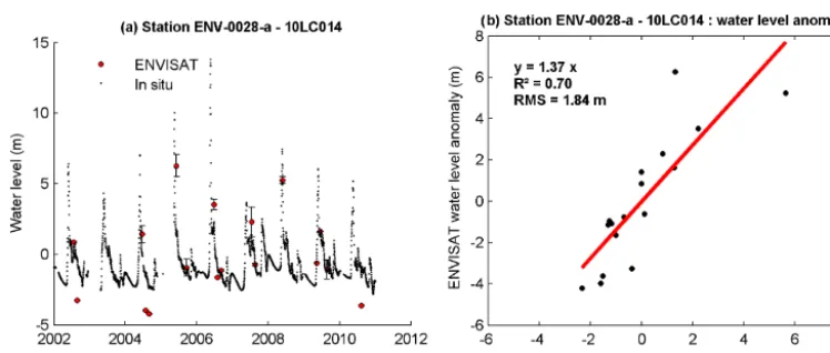
lev-Figure 8.Altimetry-based water levels from 2002 to 2010 compared to in situ water levels for the station 0439-a located in the centre of the Mackenzie Delta(a)using ENVISAT mission and(b)water level anomaly with statistic parameters.

els are much higher, with 9 m on average, but reach 12 m during the 2006 extreme event (Fig. 8a). Water level time se-ries were constructed only for ENVISAT mission since for the two others (ERS-2 and SARAL), altimetry water levels were not consistent, exhibiting values around 70 m. There-fore, water levels determined by altimetry and water levels from in situ gauges have a difference, which is probably ex-plained by the distance between virtual stations and in situ gauges (16.31 km) since the slope is about−0.02 m km−1in the Delta (Hill et al., 2001). Moreover, the seasonal cyclic thawing and freezing of the active layer causes cyclic set-tlement and heave at decimetre levels, estimated to 20 cm (Szostak-Chrzanowski, 2013).

5.3 Time series of surface water storage anomalies in the Mackenzie Delta

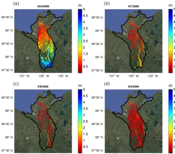
The minimum water level of each inundated pixel was de-termined over the observation period. Maps of 8-day surface water levels were created after subtracting the minimum wa-ter level to wawa-ter level at timet, using MODIS-based flood extent and altimetry-derived water levels in the entire delta from June to September. Example of water level maps are presented for 2006 at 4 different dates (in June, July, August and September), characterized as an historic flood (Fig. 9).

Over the study period, water level maps show a realistic spatial pattern with a gradient of water level from south to north, consistent with flow direction in the delta. In Fig. 9a, in June 2006, for example, water levels are higher (about 5 m) upstream than downstream (about 0.5 m). The surface wa-ter storage reaches its maximal extent in June (Fig. 9a) and then decreases during the following months, reaching 1 m in September in the entire delta (Fig. 9b, c and d).

The time series of surface water volume variations was es-timated from 2000 to 2010 and then from 2013 to 2015, be-tween June and September, following a similar approach to that in Frappart et al., 2012 (Fig. 10). Surface water storage

was estimated from 2000 to 2003 using ERS-2 data, from 2003 to 2010 using ENVISAT data and from 2013 to 2015 using SARAL. Between 2010 and 2013, surface water stor-age could not be estimated due to lack of RA data over the delta. The impact of the presence of a virtual station located in the upstream part of the delta and the inclusion of ERS-2 data on our satellite-based surface water volume estimation were assessed. For ERS-2 and SARAL data, no virtual sta-tion was created in the upstream part due to unreliable water levels in the upstream part of the delta. During the SARAL observation period, in situ water levels from 10LC014 station were used. One curve corresponds to surface water volume with virtual stations in the upstream part of the delta (2002– 2015; red) and another one without virtual stations in the up-stream part of the delta (2000–2015; green). Correlations be-tween river discharges and surface water volumes with and without (2002–2015) upstream virtual stations are the same (0.66). In the presence of a virtual station in the upstream part of the Mackenzie, the water volume decreases by∼0.3 km3 on average (Fig. 10). The correlation is lower (0.63) when ERS-2 data are included in the analysis (2000–2015). The integration of ERS-2 data has a lower accuracy and slightly decreases the correlation between water storage and flux.

Figure 9.Water level maps in the Mackenzie Delta in 2006 (historic flood) obtained by combining inundated surfaces determined using MODIS images with altimetry-derived water levels(a)in June,(b)in July,(c)in August and(d)in September.

Figure 10.Surface water volume from 2000 to 2015, determined by combining inundated surfaces from MODIS with altimetry data; 167 red points correspond to surface water volume obtained with a virtual station located in the upstream part of the Delta, green points to surface water volume without a virtual station located in the up-stream part of the Delta. The Mackenzie River Delta discharges at 10LC014 gauge station appear in blue.

6 Discussion

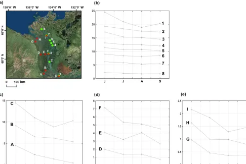
Figure 11.Temporal and spatial variations of surface water levels (in metres) in the Mackenzie Delta.(a)Location of virtual stations used to analyse spatial variations; green dots are corresponding to latitudinal variations along the Mackenzie River (from number 1 to 8) and red triangles are corresponding to longitudinal variations at three different latitudes (letters from A to I).(b)Surface water level time series along the Mackenzie River at different latitudes. Panels(c–e)show surface water levels time series at three different latitudes with three virtual stations at each latitude to analyse longitudinal spatial variations.

of extreme surface water surface area and the average water surface area duration from 2000 to 2015 were estimated for the large historic flood that occurred in 2006 (Fig. 3e) and for the minimal flood that occurred in 2010 (Fig. 3f). The whole Mackenzie Delta was practically covered in water in 2006, whereas large areas, especially in the downstream part of the delta, were not inundated in 2010 (Fig. 3f).

6.2 Spatio-temporal dynamics of surface water levels in the Mackenzie delta

For all stations and RA missions, a strong seasonal cycle can be seen, with a maximum water level reached in June after the spring ice break-up and snow melt that decreases to reach a minimal value in September, in good accordance with the hydrological cycle of the Mackenzie Delta. The delta is frozen from October to May, and during spring–early summer the freshwater meets an ice dam that was formed in winter, which provokes river discharge variations from 5000 m3 to 25 000 m3 on average (http://wateroffice.ec.gc.

ca/, Fig. 1b). Then, these important variations provoke water level increases and significant floods each year in the delta. However, water level variations as revealed from RA are not equal over the delta. In the upstream part, variations are 9 m on average, 4 m in the centre and 3 m in the downstream part of the Mackenzie Delta.

flooding that occurs in June clearly appears for all the sta-tions, the secondary peak of August–September is not well marked for all the stations. This could be due to either local differences in the hydrodynamics of the river or due to the low temporal frequency of acquisition of the altimeters that is not sufficient to fully capture all specificities of the hy-drological cycle (see Biancamaria et al., 2017 for instance). Latitudinal differences can also be noticed (Fig. 11c). Larger annual amplitudes of water levels can be observed in the Mackenzie River than over its tributaries. The second flood event occurs earlier in the central part (August) than in the western and eastern parts (September).

6.3 Spatio-temporal dynamics of surface water storage The spatio-temporal dynamics of surface water storage is presented in Fig. 9 for 2006. A strong upstream–downstream gradient of water levels can be observed in June with wa-ter levels ranging 0 to 5 m from north to south (Fig. 9a). It strongly decreases in July (0 to 1.5 m in Fig. 9b) and does not appear in August (Fig. 9c) and September (Fig. 9d). For these two later months, differences in water levels are more homogeneous of the whole delta (except in a region located around 135◦W and between 68◦N and 68◦300N in August). Our results were compared to the ones estimated by Emmerton et al. (2007) under the assumption of a stor-age change as a rectangular water layer added to the averstor-age low-water volume for a stage variation from 1.231 m above sea level during a low-water period and 5.636 m above sea level during peak flooding. Using this approach, Emmerton et al. (2007) found an increase in water volume of 14.14 km3 over the floodplains and 7.68 km3 over the channels. With our method, maximal water volume is around 9.6 km3on av-erage and can reach 14 km3. As can be seen in Fig. 11, water levels present a strong decreasing gradient of amplitude over the delta towards the mouth and are, on average, lower than 5.636 m from Emmerton et al. (2007). The difference of ap-proaches is likely to account for such discrepancy. The com-parison between storage and flux (discharge) exhibits quite a good correlation (R=0.66 with no time-lag) between these two quantities. Several studies demonstrated that there are no linear relationships among surface water extent, surface wa-ter volume and river discharge due to the presence of flood-plains non-connected to the river (e.g. Frappart et al., 2005; Heimhuber et al., 2017). Due to the small area of the non-connected lakes present in the Mackenzie delta, they are de-tected in our approach based on the use of MODIS images at 500 m of spatial resolution, as mixture areas (except during the June flood event where almost all the delta is inundated and all the flooded areas are connected to the river). Only the floodplains connected to river are considered in this study.

7 Conclusion

This study provides surface water estimates (permanent wa-ter of rivers, lakes and inundated surfaces connected to the rivers) dynamics both in extent and storage in the Macken-zie Delta from 2000 to 2015 using MODIS images at 500 m of spatial resolution and altimetry-based water levels. Sur-face water exhibits a maximal extent in the beginning of June and decreases to reach a minimal value in Septem-ber. In June, the extent of water surface area is on aver-age about 9600 km2 . The highest value was observed in 2006 (∼14 284 km2), during the historic flood described by Beltaos and Carter (2009). Despite the lower resolution of MODIS images in comparison with Landsat-8 images, sur-face water extent estimates are quite similar when using both sensors over the river channels and the floodplains, with an underestimation of 20 % found for MODIS. But the numer-ous small lakes present in the Mackenzie Delta are not de-tected using MODIS. Nevertheless, the MODIS-based inun-dation product provides important information on flooding patterns along the hydrological cycle (flood events of June and August–September).

Virtual stations, or river–lake cross sections, have been created across the Mackenzie Delta for the three radar altime-try missions (ERS-2, 1993–2003; ENVISAT, 2002–2010; SARAL, since 2013). Due to the lack of valid data acquired in interferometry SAR mode by Cryosat-2, no information on surface water levels is available in 2011 and 2012. The water levels determined by altimetry at those stations have been validated with in situ river levels, with good correlation coefficients (> 0.8) for the three missions. The dense network of altimetry virtual stations composed of 22 stations for ERS-2, 27 for ENVISAT and 24 for SARAL allowed the analysis of the spatio-temporal variations of water levels across the delta.

The combination between land water extent determined by MODIS imagery and the water levels derived from altimetry permitted estimation of surface water storage variations in the Mackenzie Delta at 8-day temporal resolution. Maps of surface water levels showed a clear upstream–downstream gradient in June that decreases with time. Temporal varia-tions in surface water volume calculated from 2000 to 2010 and from 2012 to 2015 showed a maximal volume in June (on average 9.6 km3)and a minimal volume in September (about 0.1 km3). A relatively strong correlation was found between surface water volume and the Mackenzie River discharges (R=0.66).

MODIS images, (ii) the relatively coarse spatial resolution of MODIS images, and (iii) the coarse coverage of altime-try tracks. They can be overcome (i) using SAR images for flood extent monitoring as in Frappart et al. (2005), (ii) us-ing images with a higher spatial resolution, and (iii) combus-ing information on the different altimetry missions orbiting si-multaneously. The recent launches of Sentinel-1, Sentinel-2 and Sentinel-3 offer new opportunities for flood extent mon-itoring at higher spatial (from 10 to 300 m) and temporal (a few days) resolutions. Associated with aquatic colour ra-diometry (Mouw et al., 2015), the approach developed here should provide useful information for the study of fluvial par-ticle transport along the river-to-coastal ocean continuum and its potential impacts on ecosystems.

Data availability. Surface water extent, level and storage were esti-mated in the Mackenzie Delta, Canadian Northern Territories, using multi-sensor satellite observations. Surface water area extents were estimated from 2000 to 2015 using MODIS Terra reflectances (8-day mosaic) at 500 m of spatial resolutions based on the Sakamoto et al. (2007) approach. Water levels were estimated using radar al-timetry data from ERS-2 (1995–2003), ENVISAT (2003–2010) and SARAL (2013–2016). In total, 22, 27 and 24 virtual stations were built under the ground-tracks of these missions on their nominal or-bit using the Multi-mission Altimetry Processing Software (MAPS) (Frappart et al., 2015b). Monthly surface water storage changes were obtained combining the two former datasets following the ap-proach proposed in Frappart et al. (2006, 2012) on the common pe-riod of availability of the datasets. These datasets will be soon avail-able on Hydroweb (http://hydroweb.theia-land.fr/). If you would like to access them before they are published here, you can con-tact Cassandra Normandin ([email protected]) and Frédéric Frappart ([email protected]).

Supplement. The supplement related to this article is available online at: https://doi.org/10.5194/hess-22-1543-2018-supplement.

Competing interests. The authors declare that they have no conflict of interest.

Acknowledgements. This study was supported by an internship grant from LabEX Côte (Université de Bordeaux) and a PhD grant from Ministère de l’Enseignement Supérieur et de la Recherche and also by the CNES TOSCA CTOH grant. The authors also thank David Doxaran for fruitful discussion.

Edited by: Florian Pappenberger Reviewed by: two anonymous referees

References

Alsdorf, D. E., Rodríguez, E., and Lettenmaier, D. P.: Measur-ing surface water from space, Rev. Geophys., 45, RG2002, https://doi.org/10.1029/2006RG000197, 2007.

Baup, F., Frappart, F., and Maubant, J.: Combining high-resolution satellite images and altimetry to estimate the vol-ume of small lakes, Hydrol. Earth Syst. Sci., 18, 2007–2020, https://doi.org/10.5194/hess-18-2007-2014, 2014.

Beltaos, S. and Carter, T.: Field studies of ice breakup and jamming in the Mackenzie Delta, St John’s, Newfoundland and Labrador, CGU HS Committee on River Ice Processes and the Environ-ment 15th Workshop on River Ice St. John’s, Newfoundland and Labrador, 15–17 June 2009.

Beltaos, S., Carter, T., and Rowsell, R.: Measurements and analy-sis of ice breakup and jamming characteristics in the Macken-zie Delta, Canada, Cold Reg. Sci. Technol., 82, 110–123, https://doi.org/10.1016/j.coldregions.2012.05.013, 2012. Biancamaria, S., Frappart, F., Leleu, A.-S., Marieu, V., Blumstein,

D., Desjonquères, J.-D., Boy, F., Sottolichio, A., and Valle-Levinson, A.: Satellite radar altimetry elevations performance over a 200 m wide river: Evaluation over the Garonne River, Adv. Space Res., 59, 128–146, 2017.

Birkett, C. M.: The contribution of TOPEX/POSEIDON to the global monitoring of climatically sensitive lakes, J. Geophys. Res., 100, 179–204, 1995.

Cazenave, A., Bonnefond, P., Dominh, K., and Schaeffer, P.: Caspian Sea level from Topex-Poseidon altimetry: Level now falling, Geophys. Res. Lett., 24, 881–884, https://doi.org/10.1029/97GL00809, 1997.

Crétaux, J.-F., Jelinski, W., Calmant, S., Kouraev, A., Vuglinski, V., Bergé-Nguyen, M., Gennero, M.-C., Nino, F., Abarca Del Rio, R., Cazenave, A., and Maisongrande, P.: SOLS: A lake database to monitor in the Near Real Time water level and storage varia-tions from remote sensing data, Adv. Space Res., 47, 1497–1507, https://doi.org/10.1016/j.asr.2011.01.004, 2011a.

Crétaux, J.-F., Bergé-Nguyen, M., Leblanc, M., and Abarca Del Rio, R.: Flood Mapping Inferred From Remote Sensing Data, Fifteenth International Water Technology Conference, IWTC-15 2011, Alexandria, Egypt, 2011b.

Crétaux, J. F., Nielsen, K., Frappart, F., Papa, F., Calmant, S., and Benveniste, J.: Hydrological applications of satellite altimetry: rivers, lakes, man-made reservoirs, inundated areas, in: Satellite Altimetry Over Oceans and Land Surfaces, edited by: Stammer, D. and Cazenave, A., 644 pp., CRC press, 2017.

Emmerton, C. A., Lesack, L. F. W., and Marsh, P.: Lake Abundance, potential water storage, and habitat distribution in the Mackenzie River Delta, western Canadian Arctic, Water Resour. Res., 43, W05419, https://doi.org/10.1029/2006WR005139, 2007. Emmerton, C. A., Lesack, L. F. W., and Vincent, W. F.: Nutrient and

organic matter patterns across the Mackenzie River, estuary and shelf during the seasonal recession of sea-ice, J. Mar. Syst., 74, 741–755, https://doi.org/10.1016/j.jmarsys.2007.10.001, 2008. Frappart, F., Seyler, F., Martinez, J. M., Léon, J. G., and

Cazenave, A.: Floodplain water storage in the Negro River basin estimated from microwave remote sensing of inundation area and water levels, Remote Sens. Environ., 99, 387–399, https://doi.org/10.1016/j.rse.2005.08.016, 2005.

validation over the Amazon basin, Remote Sens. Environ., 100, 252–264, https://doi.org/10.1016/j.rse.2005.10.027, 2006a. Frappart, F., Minh, K. D., L’Hermitte, J., Cazenave, A.,

Ramil-lien, G., Le Toan, T., and Mognard-Campbell, N.: Wa-ter volume change in the lower Mekong from satellite al-timetry and imagery data, Geophys. J. Int., 167, 570–584, https://doi.org/10.1111/j.1365-246X.2006.03184.x, 2006b. Frappart, F., Papa, F., Güntner, A., Werth, S., Ramillien, G., Prigent,

C., Rossow, W. B., and Bonnet, M.-P.: Interannual variations of the terrestrial water storage in the Lower Ob’ Basin from a multisatellite approach, Hydrol. Earth Syst. Sci., 14, 2443–2453, https://doi.org/10.5194/hess-14-2443-2010, 2010.

Frappart, F., Papa, F., Santos da Silva, J., Ramillien, G., Pri-gent, C., Seyler, F., and Calmant, S.: Surface freshwa-ter storage and dynamics in the Amazon basin during the 2005 exceptional drought, Environ. Res. Lett., 7, 044010, https://doi.org/10.1088/1748-9326/7/4/044010, 2012.

Frappart, F., Papa, F., Malbeteau, Y., León, J., Ramillien, G., Prigent, C., Seoane, L., Seyler, F., and Calmant, S.: Surface Freshwater Storage Variations in the Orinoco Floodplains Us-ing Multi-Satellite Observations, Remote Sens., 7, 89–110, https://doi.org/10.3390/rs70100089, 2015a.

Frappart, F., Papa, F., Marieu, V., Malbeteau, Y., Jordy, F., Calmant, S., Durand, F., and Bala, S.: Preliminary As-sessment of SARAL/AltiKa Observations over the Ganges-Brahmaputra and Irrawaddy Rivers, Mar. Geod., 38, 568–580, https://doi.org/10.1080/01490419.2014.990591, 2015b. Frappart, F., Legrésy, B., Niño, F., Blarel, F., Fuller, N., Fleury,

S., Birol, F., and Calmant, S.: An ERS-2 altimetry repro-cessing compatible with ENVISAT for long-term land and ice sheets studies, Remote Sens. Environ., 184, 558–581, https://doi.org/10.1016/j.rse.2016.07.037, 2016.

Fu, L.-L. and Cazenave, A. (Eds.): Satellite altimetry and earth sciences: a handbook of techniques and applications, Academic Press, San Diego, 2001.

Goulding, H. L., Prowse, T. D., and Bonsal, B.: Hydroclimatic controls on the occurrence of break-up and ice-jam flooding in the Mackenzie Delta, NWT, Canada, J. Hydrol., 379, 251–267, https://doi.org/10.1016/j.jhydrol.2009.10.006, 2009a.

Goulding, H. L., Prowse, T. D., and Beltaos, S.: Spatial and temporal patterns of break-up and ice-jam flooding in the Mackenzie Delta, NWT, Hydrol. Process., 23, 2654–2670, https://doi.org/10.1002/hyp.7251, 2009b.

Heimhuber, V., Tulbure, M. G., and Broich, M.: Modeling mul-tidecadal surface water inundation dynamics and key drivers on large river basin scale using multiple time series of Earth-observation and river flow data, Water Resour. Res., 53, 1251– 1269, https://doi.org/10.1002/2016WR019858, 2017.

Hill, P. R., Lewis, C. P., Desmarais, S., Kauppaymuthoo, V., and Rais, H.: The Mackenzie Delta: sedimentary processes and facies of a high-latitude, fine-grained delta, Sedimentology, 48, 1047– 1078, https://doi.org/10.1046/j.1365-3091.2001.00408.x, 2001. Holmes, R. M., McClelland, J. W., Peterson, B. J., Tank, S. E.,

Bulygina, E., Eglinton, T. I., Gordeev, V. V., Gurtovaya, T. Y., Raymond, P. A., Repeta, D. J., Staples, R., Striegl, R. G., Zhuli-dov, A. V., and Zimov, S. A.: Seasonal and Annual Fluxes of Nutrients and Organic Matter from Large Rivers to the Arctic Ocean and Surrounding Seas, Estuaries Coasts, 35, 369–382, https://doi.org/10.1007/s12237-011-9386-6, 2012.

Huete, A. R., Liu, H. Q., Batchily, K., and van Leeuwen, W.: A comparison of vegetation indices over a global set of TM images for EOS-MODIS, Remote Sens. Environ., 59, 440–451, 1997. Klein, I., Gessner, U., Dietz, A. J., and Kuenzer, C.: Global

Water-Pack – A 250 m resolution dataset revealing the daily dynamics of global inland water bodies, Remote Sens. Environ., 198, 345– 362, https://doi.org/10.1016/j.rse.2017.06.045, 2017.

Lesack, L. F. W. and Marsh, P.: River-to-lake connectivi-ties, water renewal, and aquatic habitat diversity in the Mackenzie River Delta, Water Resour. Res., 46, W12504, https://doi.org/10.1029/2010WR009607, 2010.

Macdonald, R. W. and Yu, Y.: The Mackenzie Estuary of the Arc-tic Ocean, in Estuaries, vol. 5H, edited by: P. J. Wangersky, 91–120, Springer-Verlag, Berlin/Heidelberg, available at: http: //link.springer.com/10.1007/698_5_027 (last access: 14 Decem-ber 2016), 2006.

Mouw, C. B., Greb, S., Aurin, D., DiGiacomo, P. M., Lee, Z., Twar-dowski, M., Binding, C., Hu, C., Ma, R., Moore, T., Moses, W., and Craig, S. E.: Aquatic color radiometry remote sensing of coastal and inland waters: Challenges and recommendations for future satellite missions, Remote Sens. Environ., 160, 15–30, https://doi.org/10.1016/j.rse.2015.02.001, 2015.

Muhammad, P., Duguay, C., and Kang, K.-K.: Monitoring ice break-up on the Mackenzie River using MODIS data, The Cryosphere, 10, 569–584, https://doi.org/10.5194/tc-10-569-2016, 2016.

Ogilvie, A., Belaud, G., Delenne, C., Bailly, J.-S., Bader, J.-C., Oleksiak, A., Ferry, L., and Martin, D.: Decadal monitoring of the Niger Inner Delta flood dynamics using MODIS optical data, J. Hydrol., 523, 368–383, https://doi.org/10.1016/j.jhydrol.2015.01.036, 2015.

Papa, F., Prigent, C., Aires, F., Jimenez, C., Rossow, W. B., and Matthews E.: Interannual variability of surface water extent at the global scale, 1993–2004, J. Geophys. Res., 115, D12111, https://doi.org/10.1029/2009JD012674, 2010.

Pekel, J., Cottam, A., Gorelick, N., and Belward, A. S.: High resolu-tion mapping of global surface water and its long-term changes, Nature, 540, 418–422, https://doi.org/10.1038/nature20584, 2016

Peterson, B. J., Holmes, R. M., McClelland, J. W., Vörös-marty, C. J., Lammers, R. B., Shiklomanov, A. I., Shik-lomanov, I. A., and Rahmstorf, S.: Increasing River Dis-charge to the Arctic Ocean, Science, 298, 2171–2173, https://doi.org/10.1126/science.1077445, 2002.

Rees, W. G.: Physical principles of remote sensing, Cambridge Uni-versity press, 460 pp., 2013.

Sakamoto, T., Van Nguyen, N., Kotera, A., Ohno, H., Ishit-suka, N., and Yokozawa, M.: Detecting temporal changes in the extent of annual flooding within the Cambodia and the Vietnamese Mekong Delta from MODIS time-series imagery, Remote Sens. Environ., 109, 295–313, https://doi.org/10.1016/j.rse.2007.01.011, 2007.

Santos da Silva, J., Calmant, S., Seyler, F., Rotunno Filho, O. C., Cochonneau, G., and Mansur, W. J.: Water levels in the Amazon basin derived from the ERS 2 and ENVISAT radar altimetry missions, Remote Sens. Environ., 114, 2160–2181, https://doi.org/10.1016/j.rse.2010.04.020, 2010.

Pro-cess., 11, 1427–1439, https://doi.org/10.1002/(SICI)1099-1085(199708)11:10<1427::AID-HYP473>3.0.CO;2-S, 1997. Squires, M. M., Lesack, L. F. W., Hecky, R. E., Guildford, S. J.,

Ramlal, P., and Higgins, S. N.: Primary Production and Carbon Dioxide Metabolic Balance of a Lake-Rich Arctic River Flood-plain: Partitioning of Phytoplankton, Epipelon, Macrophyte, and Epiphyton Production Among Lakes on the Mackenzie Delta, Ecosystems, 12, 853–872, https://doi.org/10.1007/s10021-009-9263-3, 2009.

Stocker, T. F. and Raible, C. C.: Water cycles shifts gear, Nature, 434, 830–831, 2005.

Szostak-Chrzanowski, A.: Study of Natural and Man-induced Ground Deformation in MacKenzie Delta Region, Acta Geodyn. Geomater., 11, 117–123, https://doi.org/10.13168/AGG.2013.0060, 2013.

Tulbure, M. G., Broich, M., Stehman, S. V., and Kommareddy, A.: Surface water extent dynamics from the three decades of sea-sonally continuous Landsat time series at subcontinental scale in a semi-arid region, Remote Sens. Environ., 178, 142–157, https://doi.org/10.1016/j.rse.2016.02.034, 2016.

Ulaby, F. T., Moore, R. K., and Fung, A. K.: Microwave mote sensing: Active and passive, Volume 1 – Microwave re-mote sensing fundamentals and radiometry, available at: https: //ntrs.nasa.gov/search.jsp?R=19820039342 (last access: 15 De-cember 2016), 1981.

Verpoorter, C., Kutser, T., Seekell, D. A., and Tranvik, L. J.: A global inventory of lakes based on high-resolution satellite imagery, Geophys. Res. Lett., 41, 6396–6402, https://doi.org/10.1002/2014GL060641, 2014.

Verron, J., Sengenes, P., Lambin, J., Noubel, J., Steunou, N., Guillot, A., Picot, N., Coutin-Faye, S., Sharma, R., Gairola, R. M., Murthy, D. V. A. R., Richman, J. G., Griffin, D., Pascual, A., Rémy, F., and Gupta, P. K.: The SARAL/AltiKa Altimetry Satellite Mission, Mar. Geod., 38, 2– 21, https://doi.org/10.1080/01490419.2014.1000471, 2015. Wang, M. and Shi, W. Estimation of ocean contribution at the

MODIS near-infrared wavelengths along the east coast of the U.S.: Two case studies, Geophys. Res. Lett., 32, L13606, https://doi.org/10.1029/2005GL022917, 2005.

Xiao, X., Boles, S., Liu, J., Zhuang, D., Frolking, S., Li, C., Salas, W., and Moore, B.: Mapping paddy rice agriculture in southern China using multi-temporal MODIS images, Remote Sens. En-viron., 95, 480–492, https://doi.org/10.1016/j.rse.2004.12.009, 2005