State and parameter estimation of two land surface models using the ensemble Kalman filter and the particle filter

https://doi.org/10.5194/hess-21-4927-2017 © Author(s) 2017. This work is distributed under the Creative Commons Attribution 3.0 License.

State and parameter estimation of two land surface models using the

ensemble Kalman filter and the particle filter

Hongjuan Zhang1,2, Harrie-Jan Hendricks Franssen1,2, Xujun Han1,2, Jasper A. Vrugt3,4, and Harry Vereecken1,2 1_{Forschungszentrum Jülich, Agrosphere (IBG 3), Jülich, Germany}

2_{Centre for High-Performance Scientific Computing in Terrestrial Systems: HPSC TerrSys, Forschungszentrum Jülich,} Jülich, Germany

3_{Department of Civil and Environmental Engineering, University of California Irvine, Irvine, USA} 4_{Department of Earth Systems Science, University of California Irvine, Irvine, USA}

Correspondence to:Hongjuan Zhang ([email protected]) Received: 25 January 2016 – Discussion started: 23 February 2016

Revised: 24 May 2017 – Accepted: 19 July 2017 – Published: 29 September 2017

Abstract.Land surface models (LSMs) use a large cohort of parameters and state variables to simulate the water and en-ergy balance at the soil–atmosphere interface. Many of these model parameters cannot be measured directly in the field, and require calibration against measured fluxes of carbon dioxide, sensible and/or latent heat, and/or observations of the thermal and/or moisture state of the soil. Here, we eval-uate the usefulness and applicability of four different data assimilation methods for joint parameter and state estima-tion of the Variable Infiltraestima-tion Capacity Model (VIC-3L) and the Community Land Model (CLM) using a 5-month calibration (assimilation) period (March–July 2012) of areal-averaged SPADE soil moisture measurements at 5, 20, and 50 cm depths in the Rollesbroich experimental test site in the Eifel mountain range in western Germany. We used the EnKF with state augmentation or dual estimation, respec-tively, and the residual resampling PF with a simple, sta-tistically deficient, or more sophisticated, MCMC-based pa-rameter resampling method. The performance of the “cal-ibrated” LSM models was investigated using SPADE wa-ter content measurements of a 5-month evaluation period (August–December 2012). As expected, all DA methods en-hance the ability of the VIC and CLM models to describe spatiotemporal patterns of moisture storage within the va-dose zone of the Rollesbroich site, particularly if the max-imum baseflow velocity (VIC) or fractions of sand, clay, and organic matter of each layer (CLM) are estimated jointly with the model states of each soil layer. The differences between the soil moisture simulations of VIC-3L and CLM are much

larger than the discrepancies among the four data assimila-tion methods. The EnKF with state augmentaassimila-tion or dual es-timation yields the best performance of VIC-3L and CLM during the calibration and evaluation period, yet results are in close agreement with the PF using MCMC resampling. Over-all, CLM demonstrated the best performance for the Rolles-broich site. The large systematic underestimation of water storage at 50 cm depth by VIC-3L during the first few months of the evaluation period questions, in part, the validity of its fixed water table depth at the bottom of the modeled soil do-main.

1 Introduction and scope

conceptual-ize and aggregate the complex, spatially distributed, and in-terrelated (bio)physical, chemical, and ecological processes that govern the exchange of mass, energy, and momentum between the land surface and the atmosphere. This approach simplifies considerably the topology of the land surface sys-tem, and reduces to much lower dimensions its state and parameter space. The consequence of this process aggrega-tion and simplificaaggrega-tion is however that the LSM parameters often do not represent directly measurable entities, and in-stead must be estimated via calibration by fitting the model against measured data records of soil moisture, soil tempera-ture, and/or CO2, water vapor, and/or energy fluxes across a range of biomes and timescales. These measurements are of crucial importance to quantify properly LSM parameter and predictive uncertainty, and to identify poorly represented or missing processes (Williams et al., 2009; Bonan, 2008).

Many of the parameters of a LSM are model dependent and therefore difficult to transfer between different land sur-face schemes. Nevertheless, all LSMs use soil hydraulic, vegetation, and thermal parameters to describe heat trans-port, water flow, and root water uptake (canopy transpira-tion) in the variably saturated soil domain, and share a re-flection coefficient (also known as surface albedo) to calcu-late the reflected shortwave radiation. Two main approaches exist to determine the hydraulic and thermal properties of the considered soil domain. Some LSMs such as the Com-munity Land Model (CLM) use basic soil data (soil tex-ture and organic matter fraction) to estimate hydraulic and thermal parameters via pedotransfer functions (Oleson et al., 2013; Han et al., 2014; Vereecken et al., 2016). Other land surface schemes such as the Variable Infiltration Capacity Model (VIC) (Liang et al., 1994; Gao et al., 2010) expect users to specify values for the hydraulic and thermal param-eters. Pedotransfer functions are particularly useful in large-scale application of CLM as they simplify tremendously soil hydraulic characterization. Nevertheless, soil hydraulic pa-rameter values derived from pedotransfer functions are sub-ject to considerable uncertainty, and might therefore not ac-curately describe soil water movement and storage, particu-larly at larger spatial scales. What is more, (measurement) errors of the atmospheric forcing (e.g., wind speed, tempera-ture, radiation, vapor pressure deficit, and precipitation) and errors in the auxiliary model input (e.g., topographic proper-ties, vegetation characteristics) further enhance LSM predic-tion uncertainty.

In the past decades, many different search and optimiza-tion methods have been developed for automatic calibraoptimiza-tion of dynamic system models. Of these, Bayesian methods have found widespread application and use in Earth systems mod-eling due to their innate ability to treat, at least in princi-ple, model input (forcing), output (forecast), parameter, and structural errors. The Bayesian approach relaxes the assump-tion of a single optimum parameter value in favor of a pos-terior parameter and forecast distribution which summarizes the coordinated impact of different uncertainties on the

mod-eling results. Yet, general-purpose methods such as DREAM (Vrugt et al., 2008, 2009; Vrugt, 2016) require a relatively large number of LSM evaluations to estimate parameter and forecast uncertainty. This can pose significant computational challenges for CPU-intensive and parameter-rich LSMs, and complicates treatment of input data uncertainty via latent variables (e.g., Vrugt et al., 2008).

Data assimilation offers an attractive alternative as a gen-eral framework to account for LSM parameters, input, out-put, and other sources of uncertainty to take advantage of all available ground-based, airborne, or spaceborne observa-tions to improve the compliance between numerical models and corresponding data. This approach enables joint estima-tion of model state variables and parameters and simplifies treatment of forcing data errors (Liu and Gupta, 2007). Many different studies published in the hydrologic literature have demonstrated the benefits of parameter estimation in the con-text of data assimilation for soil moisture characterization (e.g., Montzka et al., 2011; Lee et al., 2014), rainfall–runoff (e.g., Moradkhani et al., 2005b; Vrugt et al., 2005a) and land surface modeling (e.g., Pauwels et al., 2009).

Data assimilation methods merge uncertain observations with predictions (output) of imperfect models to optimally estimate the state of a dynamical system. The prototype of this method, the Kalman filter (KF), was developed in the 1960s by Rudy Kalman for optimal control of linear dynam-ical systems (Kalman, 1960). The KF is a maximum like-lihood estimator of the dynamic state of the system if the model error and measurement error distributions are (multi-variate) normal. For nonlinear dynamical models this Gaus-sian assumption is not generally valid, and the KF will not give a maximum likelihood state estimate. The ensemble Kalman filter, or EnKF, is a stochastic generalization of the KF to nonlinear system models, in which the evolution of the model error covariance matrix is derived from a finite set of state realizations (Evensen, 1994). The use of this Monte Carlo ensemble not only makes possible state estimation for complex system models, but also enables the explicit treat-ment of different sources of modeling error. Two decades on from its inception, the EnKF has received operational sta-tus in real-time weather, tsunami, and flood prediction sys-tems (amongst others) due to its proven ability to enhance a model’s forecast skill and characterize accurately prediction uncertainty.

investigated by many different authors in the water resources literature. Most of these publications use synthetic (or twin) experiments with assimilation of artificially generated data. Examples include studies with simulated measurements of the groundwater table depth or hydraulic head (Franssen and Kinzelbach, 2008; Bailey and Baù, 2012; Kurtz et al., 2014; Shi et al., 2014; Song et al., 2014; Tang et al., 2015), dis-charge/streamflow (Bailey and Baù, 2012; Moradkhani et al., 2012; Vrugt et al., 2013; Rasmussen et al., 2015), groundwa-ter temperature (Kurtz et al., 2014), soil moisture (Wu and Margulis, 2011; Plaza et al., 2012; Erdal et al., 2014; Shi et al., 2014; Song et al., 2014; Pasetto et al., 2015), bright-ness temperature from passive remote sensing (Montzka et al., 2013; Han et al., 2014), and contaminant concentration (Gharamti et al., 2013). These studies use a variety of differ-ent methods for joint parameter and state estimation, among which the EnKF (Franssen and Kinzelbach, 2008; Wu et al., 2011; Gharamti et al., 2013; Erdal et al., 2014; Kurtz et al., 2014; Shi et al., 2014; Pasetto et al., 2015), the iterative EnKF (Song et al., 2014), the extended KF (Pauwels et al., 2009), the local ensemble transform KF (Han et al., 2014), the en-semble transform KF (Rasmussen et al., 2015), and the nor-mal score EnKF (Tang et al., 2015).

The overarching conclusion from the body of synthetic ex-periments is that the joint estimation of parameters and state variables via data assimilation enhances significantly the pre-dictive capabilities of hydrologic and land surface models. This finding is corroborated by results for real-world assim-ilation studies documented in a rapidly growing list of pub-lications and involving model structural inadequacies, mea-surement errors of the atmospheric forcing variables and cali-bration (assimilation) data, inadequate characterization of the lower boundary condition (aquifer), and uncertainty of other, auxiliary, model inputs. This includes assimilation of mea-surements of the electrical conductivity (Wu and Margulis, 2013), hydraulic head in wells (Kurtz et al., 2014; L. Shi et al., 2015), groundwater temperature (Kurtz et al., 2014), streamflow and discharge (Moradkhani et al., 2012; Y. Shi et al., 2015), active remote sensing (Pauwels et al., 2009), pas-sive brightness temperature (Qin et al., 2009), soil moisture from lysimeters (Lue et al., 2011; Wu and Margulis, 2013; Erdal et al., 2014; L. Shi et al., 2015), land surface temper-ature (Bateni and Entekhabi, 2012), and sensible and latent heat fluxes (Y. Shi et al., 2015) using methods such as the PF (Qin et al., 2009), PMCMC (Moradkhani et al., 2012), EnKF (Bateni and Entekhabi, 2012; Wu and Margulis, 2013; Erdal et al., 2014; Kurtz et al., 2014; Y. Shi et al., 2015), and the extended KF (Pauwels et al., 2009; Lue et al., 2011). De-spite this growing body of applications, relatively few stud-ies (e.g., Lue et al., 2011; Y. Shi et al., 2015) have focused on an accurate characterization of soil moisture dynamics sim-ulated by LSMs. This is particularly surprising, as root zone moisture storage modulates spatiotemporal variations in cli-mate and weather, and governs the production and health

sta-tus of crops and the organization of natural ecosystems and biodiversity (Vereecken et al., 2008).

In this paper, we evaluate the usefulness and applicabil-ity of four different data assimilation methods for joint pa-rameter and state estimation of VIC-3L and CLM using a 5-month calibration (assimilation) period of soil moisture mea-surements at 5, 20, and 50 cm depths in the Rollesbroich ex-perimental test site in the Eifel mountain range in western Germany. This grassland site is part of the TERENO net-work of observatories and has been extensively monitored since 2011 to catalog long-term ecological, social, and eco-nomic impacts of global change at regional level. We used the EnKF with state augmentation (Chen and Zhang, 2006) or dual estimation (Moradkhani et al., 2005b), respectively, and the residual resampling PF (Douc et al., 2005) with a simple, statistically deficient (Moradkhani et al., 2005a), or more so-phisticated, MCMC-based (Vrugt et al., 2013) parameter re-sampling method. The “calibrated” LSM models were tested using SPADE water content measurements from a 5-month evaluation period. To the best of our knowledge, this is only the second study after Chen et al. (2015) that compares se-quential data assimilation methods for joint parameter and state estimation of a LSM. Related work by DeChant and Moradkhani (2012) and Dumedah and Coulibaly (2013) con-sider application to the rainfall–runoff transformation of a watershed.

The three main objectives of our study may be summarized as follows: (1) to evaluate the usefulness and applicability of joint parameter and state estimation for soil moisture char-acterization with LSMs, (2) to compare the performance of four commonly used parameter and state estimation methods in their ability to predict soil moisture dynamics at different depths in the Rollesbroich experimental test site, and (3) to compare, contrast, and juxtapose the soil moisture simula-tions and predicsimula-tions of CLM and VIC.

2 Land surface models and calibration parameters LSMs simulate terrestrial biosphere fluxes of matter and energy via numerical solution of the water, energy, and carbon balance of the land surface. This includes hydro-logic processes such as soil evaporation, infiltration, sur-face runoff, canopy interception and transpiration, aquifer discharge, groundwater recharge, and precipitation (Schaake et al., 1996), and energy fluxes such as latent and sensible heat from soil, snow, surface water, and vegetated surfaces (Bertoldi, 2004). Their respective equations contain parame-ters whose values depend on global or regional distributions of vegetation and soil properties (Milly and Shmakin, 2002). The Rollesbroich site investigated herein covers an area of about 270 000 m2with grassland vegetation that is dominated by perennial ryegrass (Loliumperenne) and smooth meadow grass (Poapratensis). The limited size of our site and its rather uniform vegetation and topography justify treatment of our land surface domain as a single grid cell in a LSM with ap-parent parameters that characterize the mass and energy ex-change between the soil and atmosphere. This assumption of homogeneity is computationally convenient and also sim-plifies somewhat our subsequent mathematical notation. We conveniently write the LSM as a (nonlinear) regression func-tion, M(·), which returns a m×n matrix Y with the sim-ulated (predicted) values ofmdifferent variables (e.g., soil moisture content, latent and sensible heat fluxes) at discrete times,t∈ {1, . . ., n}, as follows:

Y←M(α,_ex0,eB,U ),e (1)

whereα= {α1, . . ., αd}is thed-vector of model parameters,

ex0signifies thek×1-vector with measured (inferred) values of the state variables of the land surface model for the domain at the start of simulation, eBdenotes the l×n control ma-trix with temporal measurements oflforcing variables (e.g., air temperature, precipitation, vapor pressure deficit, wind speed, and shortwave and longwave radiation),Uerepresents a list with auxiliary constants, variables, or properties (e.g., plant functional type, land cover, soil texture, and other vari-ables/constants) deemed necessary to simulate the water and energy balance of the land surface domain of interest, and Y=y1

1:n, . . .,ym1:n

T

, where T denotes the transpose. With-out loss of generality, we restrict the model parameters to a closed space,A, equivalent to somed-dimensional hyper-cube,α∈A∈Rd, called the feasible parameter space.

The assumption of homogeneity simplifies considerably the model definition in Eq. (1). Yet, this lumped topology might not characterize adequately real-world soil land sur-face systems that exhibit considerable spatial variations in soils, vegetation, and land properties. Such systems might necessitate distributed application of Eq. (1) via spatial dis-cretization of the considered land surface domain into differ-ent grid cells. This discretization should honor spatial vari-ations in vegetation and soil properties, and could account for small-scale (within-grid-cell) variability. Nevertheless, in

our present application of LSM we the treat the Rollesbroich site as a single grid cell with grassland vegetation and homo-geneous, but layered, soil (details to follow).

We now discuss briefly two different land surface schemes, VIC-3L and CLM, which are used to describe temporal vari-ations in soil water storage at different depths in the Rolles-broich experimental site in Germany.

2.1 The Variable Infiltration Capacity (VIC) model The VIC model is a macro-scale semi-distributed hydrolog-ical model which solves for the water and energy balance of each grid cell using explicit consideration of within-grid-cell vegetation variations. Accordingly, each grid cell is divided into land cover tiles (Liang et al., 1994, 1996; Cherkauer and Lettenmaier, 1999) and assumes constant values of the soil properties (e.g., soil texture, hydraulic conductivity, ther-mal conductivity). The total evapotranspiration, sensible heat flux, effective land surface temperature, and runoff are then obtained for each grid cell by summing over all the land cover tiles (vegetation types and bare soil) weighted by their respective fractional coverage (Gao et al., 2010). The VIC model can either be executed in a water balance mode or a water-and-energy balance mode. In this paper, we assume the latter and use a 70 cm deep soil composed of a 10 cm surface layer followed by middle and bottom layers of 20 and 40 cm, respectively. The relatively thin surface layer is used to cap-ture rapid fluctuations in soil moiscap-ture due to rainfall and bare soil evaporation, and the deepest and thickest layer summa-rizes seasonal water content dynamics and baseflow. We use herein VIC-3L and force the model with atmospheric bound-ary conditions (e.g., precipitation, wind speed, air tempera-ture, longwave and shortwave radiation, and relative humid-ity) for the Rollesbroich experimental site in Germany. In the absence of detailed information about the hydraulic proper-ties of the considered soil domain, we treat each layer’s satu-rated hydraulic conductivity, log10ks(log10(m s−1)), and the exponent of the Brooks–Corey drainage equation,β (–), as calibration parameters. What is more, we also include the in-filtration shape parameter,b(–), and the maximum baseflow velocity,Dm (mm day−1), as calibration parameters. Thus, this involves estimation ofd=8 parameters in VIC-3L for the Rollesbroich site. Appendix A summarizes the soil mod-ule of VIC-3L, including a brief description of the main pro-cesses and model parameters.

2.2 The Community Land Model (CLM)

into multiple subgrid levels. For example, a grid cell can be made up of different land cover types, each with its own re-spective patches of plant functional types (PFTs) and asso-ciated stem area index and canopy height. The first subgrid level is defined by land units (vegetated, lake, urban, glacier, and crop), each composed of a number of different columns (second subgrid level) for which separate energy and water calculations are made. Vegetated land units, as well as lakes and glaciers, use one column. Urban land uses five separate columns, and for crop land there is a distinction between ir-rigated and unirir-rigated columns, with one single crop occu-pying each column. The third subgrid level is composed of PFTs and includes bare soil. The vegetated column has 16 possible PFTs besides bare soil. For the crop column, several crop types are available. Processes such as canopy evapora-tion and transpiraevapora-tion are calculated for each individual PFT, whereas soil and snow processes are calculated at the col-umn level using areal-weighted values of the properties of the PFTs of individual patches. Note that a similar aggrega-tion approach is used by VIC-3L.

In our application of CLM to the Rollesbroich experi-mental site in Germany, we calculate soil temperature for 15 different soil layers, and simulate hydrological states and fluxes for the top 10 soil layers only. Appendix B presents a brief description of the soil module of CLM, and discusses the main parameters used. CLM is forced with atmospheric conditions (e.g., precipitation, vapor pressure deficit, wind speed, incoming shortwave and longwave radiation) using values for the model parameters and initial states, and land surface data and other physical constants and/or variables as auxiliary input. The soil hydraulic (e.g., saturated hydraulic conductivity) and thermal parameters of CLM are derived from built-in pedotransfer functions (see Eqs. B1–B4 of Ap-pendix B) using as inputs the auxiliary listUewith sand, clay, and organic matter fractions of each individual soil layer. We treat these auxiliary soil variables as unknown parameters in the present application of CLM. Thus, this involvesd=30 parameters in CLM for the Rollesbroich site.

2.3 Main differences of VIC-3L and CLM

Before we proceed, we first summarize the main differences of VIC-3L and CLM in their calculations of the water and energy balance of the land surface. In the first place, VIC-3L treats the vadose zone as a multi-layer bucket with vari-able infiltration capacity, whereas CLM uses a more physics-based description of soil water movement, storage, and asso-ciated hydrological fluxes (e.g., root water uptake) by numer-ical solution of a modified form of Richards’ equation (Zeng and Decker, 2009). A bucket model is computationally con-venient, but sacrifices important detail regarding the vertical distribution of soil water storage. The latter is a prerequi-site for characterizing accurately processes such as infiltra-tion, redistribuinfiltra-tion, root-water uptake, drainage, and ground-water recharge. We refer the interested reader to Romano

et al. (2011) for a detailed comparison of bucket type and Richards-based vadose zone flow models.

Second, VIC-3L treats the saturated and variably saturated soil domain as two separate, lumped, control volumes which are decoupled from the underlying groundwater reservoir. In other words, a fixed lower boundary condition is imposed. CLM, by contrast, simulates interactions between the mod-eled soil domain and an unconfined aquifer. The resulting water table variations of the aquifer affect soil water move-ment in the unsaturated zone via a variable recharge flux. In our application of CLM, this recharge flux emanates at the bottom of the tenth soil layer. The calculation of this recharge flux may be best explained via the use of a vir-tual soil layer, say layer 11, whose depth extends from the bottom of layer 10 to the groundwater table. If we assume hydrostatic conditions in layer 11, then we can calculate the recharge flux from layer 10 using Eq. (B9) in Appendix B. This recharge flux then changes the depth of the water table according to Eq. (B11). This equation also takes into con-sideration drainage from the water table due to topographic gradients. If the groundwater table is within the upper 10 soil layers, a drainage flux emanates from the uppermost satu-rated layer according to Eq. (B10).

Third, VIC-3L expects the user to specify values for the soil hydraulic (e.g., saturated hydraulic conductivity), ther-mal, and baseflow parameters of the first, second, and third layers of each grid cell, respectively, whereas CLM derives their counterparts (e.g., hydraulic conductivity at saturation, matric head at saturation, Clapp–Hornberger exponent B, and soil thermal conductivity) for each of the 15 soil layers using built-in pedotransfer functions.

Finally, VIC-3L allows the user to determine freely the number and thickness of the soil layers in the bucket model (the default is three layers), whereas CLM assumes a fixed thickness of each soil layer.

2.4 Selection of calibration parameters

Table 1.Description of the soil parameters of VIC-3L and CLM that are subject to inference with the different data assimilation methods using the 5-month soil moisture calibration data period of the Rollesbroich site. We list the symbol, unit, feasible range, perturbation, and domain of application of each parameter of VIC-3L and CLM. The column with the header “Perturbation” lists the statistical distributions that are used to create the initial parameter ensemble for each data assimilation algorithm. The notationN (a, b)signifies the univariate normal distribution with meanaand standard deviationb, whereasU (a, b)denotes the univariate uniform distribution betweenaandb. These perturbation distributions are centered on the best-guess parameter values of VIC-3L and CLM (see Sect. 4.2) and define together the prior parameter distribution. This prior distribution honors textural measurements of each soil layer and its dispersion is in agreement with previously published studies.

Model Parameter Description Units Ranges Perturbation Configuration

VIC-3L log10ks Saturated hydrologic conductivity log10(m s−1)b [−7,−3] N (0,1) Layer β Exponent of the Brooks–Corey drainage equation – [8, 30] U (−5,5) Layer b Infiltration shape parameter – [10−3, 0.8] U (−0.1,0.1) Profile Dm Maximum baseflow velocity mm d−1 (0, 30] U (−10,10) Profile

CLM fcl Clay fraction – [0.01, 1] U (−0.1,0.1) Layer

fsd Sand fraction – [0.01, 1] U (−0.1,0.1) Layer

fom Organic matter fraction – [0, 1] U (−0.12,0.12) Layer

a_{Note that the sand, clay, and organic matter fractions of each layer serve as input to pedotransfer functions in CLM which compute the hydraulic properties of each layer. See}

Eqs. (B2)–(B5) of Appendix B.bIn the figures of this paper, we conveniently use labels with units of m s−1_{for log} 10ks.

This makes up the prior parameter distribution and is further explained in Sect. 4.2.

Appendices A (VIC-3L) and B (CLM) summarize the main variables, processes, and equations which are used by both models to describe the storage and vertical and/or hor-izontal movement of water in the variably saturated soil do-main of the Rollesbroich site. These two appendices help to better understand the role of the different calibration parame-ters of Table 1, and will be most beneficial to readers who are rather unfamiliar with both models. Note that CLM estimates the hydraulic and thermal parameters of each soil layer from built-in pedotransfer functions (Oleson et al., 2013; Han et al., 2014) using as input the sand, clay, and organic matter fractions of each soil layer.

3 Data assimilation methods

Data assimilation methods merge uncertain observations with predictions (output) of imperfect models to optimally estimate the state and/or parameters of a dynamical system. This includes the use of four-dimensional variational data assimilation (4D-Var), EnKF, PF, and related assimilation schemes. These methods have been applied successfully to a large number of different fields for model–data fusion in the atmospheric, oceanic, biogeochemical, and hydrological sciences. We now briefly discuss the theory of four different data assimilation methods which are used herein with VIC-3L and CLM to characterize spatiotemporal soil moisture dy-namics at our experimental site.

3.1 EnKF

The EnKF was proposed by Evensen (1994) as a general-ization of the Kalman filter to nonlinear system models with many state variables. This method uses a Monte Carlo ap-proach to generate an ensemble of different model trajecto-ries from which the time evolution of the probability den-sity of the model states and related error covariances are es-timated. The EnKF uses a state-space implementation of the dynamic system model of Eq. (1) and implements the follow-ing steps (Burgers et al., 1998):

xi_t−=M(α,xi_t−1,eb

i

t−1,I)+wt, (2)

wherexi_t−is thek×1-vector of predicted values of the state variables of theith ensemble member,i= {1, . . ., N},eb

i t−1 signifies the corresponding vector (or matrix) of measured values of the forcing variables,wt denotes ak×1 process

noise vector that accounts for structural imperfections of the LSM, andtdenotes time. In our specific implementation, the state vector is made up of areal-averaged soil moisture con-tent values at three different measurement depths. What is more, the observed precipitation forcing was perturbed with a member-dependent vector of measurement errors. From the ensemble ofNstate vectors, we can calculate thek×k back-ground error covariance matrix,C, using

C= 1 N−1

XN

i=1(x

i−

t −xt)(xit−−xt), (3)

wherextdenotes thek×1 vector with ensemble mean values

of the states at time t. The m×1 vector of measured soil moisture data at time t can be written for each individual ensemble member as follows:

ˆ yi_t=

eyt+v

i

where vi

t signifies a m×1 vector of measurement

er-rors drawn randomly from a m-variate normal distribution,

Nm(0,R)with zero-mean and m×mobservation error

co-variance matrix R. We assume the soil moisture measure-ment errors at each depth to have a fixed and common vari-anceσ2, and to be uncorrelated in space and time. Thus we can write R=σ2Im, whereImsignifies them×midentity

matrix with zeros everywhere except on the main diagonal which stores values ofσ2.

We can now update the predicted state values of each en-semble member as follows:

x_ti =xi_t−+K(yˆi_t−Hxi_t−), (5) wherexi_t denotes thek×1 vector with updated estimates of the state variables (also called analysis state),Kis ak×m

matrix called the Kalman gain, and them×kmatrixH sig-nifies the measurement operator which maps the model out-put to the measurement space. It is linear for EnKF. In our present application, we observe directly the soil moisture content of respective measurement depth, and thus the ma-trixHis made up of values of zero and unity. The Kalman gain is computed as follows:

K=CHT(HCHT+R)−1, (6)

where the symbol T denotes the transpose. The updated val-ues of the states now enter Eq. (2) and are used to predict the soil moisture values at the next observation time, t=t+1, and so forth.

In some cases it might be appropriate to estimate the model parameters along with the state variables. This re-quires a slight modification to the state-space formulation of Eq. (2) as thed-vector of parameter values,α, must now vary among theN ensemble members to facilitate parame-ter estimation from the measured data. Three different ap-proaches have been published in the literature for joint es-timation of model states and parameters in the EnKF. This includes, state augmentation, dual and outer estimation. The first two approaches assume the LSM parameters to be time-variant, and infer their values sequentially along with the model states. The third approach assumes the parameters to be time-invariant, and estimates their posterior distribution in a loop outside the EnKF by maximizing the marginal likeli-hood of theN state trajectories (Vrugt et al., 2005a, 2013). We will consider herein only the first two approaches, that is, state augmentation and dual estimation, as these two methods are most CPU-efficient.

3.1.1 State augmentation

In state augmentation, thek×1 vector of state variables,xt,

the model error covariance matrixC, the measurement oper-atorH, and the Kalman gainKconsist of two separate blocks

(Franssen and Kinzelbach, 2008): x∗i=

xi αi

(7)

C∗=

Cxx CTαx Cαx Cαα

(8)

H∗=[Hx,0], (9)

where the subscriptsx andαrefer to the model states and parameters, respectively. The state vector,x∗_{, now consists}

ofk+d elements, the model error covariance matrixC∗_is

made up of four smaller matrices,Cxx,CTαx,Cαx, andCαα, and the measurement operatorH∗_includesH

xand additional values of zero. The Kalman gain matrixKis now given by K=C∗H∗T(H∗C∗H∗T +R)−1=

Cxx CTαx Cαx Cαα

HT_x 0

[Hx,0]

Cxx CTαx Cαx Cαα

HT_x 0 +R −1 =

CxxHTx(HxCxxHTx+R)−1 CαxHTx(HxCxxHTx+R)−1 = Kx Kα . (10)

This results in the following equation for the updated states and parameter values:

xi t αi t = xi_t− αit−

+

Kx(ˆyit−Hxxit−) Kα(ˆyit−Hxxit−)

. (11)

3.1.2 Dual estimation

In the dual estimation approach, the state variables and model parameters are stored in two separate vectors and updated using their own individual steps (Moradkhani et al., 2005b). The parameter values of each ensemble member are first up-dated according to

α_ti=αi_t−+Kα(yˆit−Hxxit−). (12)

Then, the updated parameter values are used with Eq. (2) to predict, for the second time, the state variables at timet, after which their values are updated via Eq. (5). This approach ne-cessitates running the LSM twice for the time period between two successive measurements, thereby doubling the required CPU time of each ensemble member for this dual estimation method compared to the state augmentation approach.

inbreeding is aggravated by the use of a relatively low num-ber of ensemble memnum-bers (small N), which results in spu-rious correlations among state variables and/or parameters, and underestimation of the spread of the ensemble. Other reasons for an insufficient ensemble spread are model struc-tural errors and the use of an underdispersed prior parameter distribution or overly small variance of the measurement er-rors of the forcing variables. Ensemble inflation methods are an effective way of ameliorating filter inbreeding (Anderson, 2007; Whitaker and Hamill, 2012). We apply the inflation al-gorithm of Whitaker and Hamill (2012) to the d parameter values of each ensemble member as follows:

α_j,ti =αj,t+ Vj Wj

α_j,ti −αj,t

, (13)

whereαj,t signifies the analysis mean (after update) of the jth parameter at timet, the scalarsVj andWj denote the

prior (before update) and analysis standard deviation of the

jth parameter (derived from ensemble), andj= {1, . . ., d}. This method promotes a parameter spread that is in agree-ment with the width of the prior parameter distribution, and is particularly important to avoid a strong underestimation of ensemble variance and associated filter inbreeding in appli-cations with relatively small ensemble sizes. As the spread is kept artificially constant, it cannot be assessed properly how data assimilation affects reduction of prediction uncertainty. In addition, it is important that the initial ensemble spread is adequate. This is a drawback of the applied inflation. 3.2 Residual resampling particle filter (RRPF) and

parameter estimation

The PF was first suggested in the research area of ob-ject recognition, robotics and target tracking (Gordon et al., 1993) and was introduced to hydrology by Moradkhani et al. (2005b). The PF differs from the EnKF in that it describes the evolving probability density function (PDF) of the LSM state variables by a set ofNrandom samples, also called par-ticles. Each particle carries a non-zero weight which deter-mines its underlying probability, and these weights are up-dated as soon as a new datum (observation) becomes avail-able. Before we proceed with a brief theoretical description of the PF we must first explicate our notation. We denote with symbol X1:t the collection of simulated values of the LSM

state variables between the first observation att=1 and the present datum,t, henceX1:t=[x1, . . .,xt] is ak×t matrix

with the LSM states at each measurement time stored as a column vector. The corresponding observations are stored in them×tmatrix,eY1:t=ey1, . . .,eyt

. Finally, we use braces,

{·}, to denote our Monte Carlo ensemble ofN particle tra-jectories,

X1₁:_:N_t , and thus

X1_t:N is ak×N matrix with sampled values of the LSM state variables at timet. The sub-sequent description of the PF follows closely the description of Vrugt et al. (2013). Interested readers are referred to this publication for further details.

If we assume the parameters to be known, then we can write the evolving posterior distribution,pα(X1:t|eY1:t), for

the state-space formulation of Eq. (2) as follows:

pα X1:t|eY1:t (14)

=

prior z }| {

pα(X1:t|eY1:t−1)

model z }| {

Mα(xt|xt−1)

likelihood function z }| {

Lα(eyt|xt)

pα(eyt|eY1:t−1) | {z } normalization constant

,

where pα X1:t−1|eY1:t−1 denotes the prior state distribu-tion,Mα(xt|xt−1)signifies the transition probability density of the state variables (=Eq. 2),Lα(eyt|xt)is the likelihood function, andpα(eyt|eY1:t−1)represents a normalization con-stant which ensures that the posterior state distribution inte-grates to unity. Equation (14) follows directly from Bayes’ law (see Appendix A of Vrugt et al., 2013), and does not use at once the data up to timet to estimatepα X1:t|eY1:t

but rather estimates the evolving system state recursively over time using some mathematical model and new incom-ing measurements. If we integrate out the state trajectory X1:t−1 from Eq. (14) then we can derive an expression for the marginal PDF of the state variables,pα xt|eY1:t, at time t:

pα xt|eY1:t=

Lα(eyt|xt)pα xt|eY1:t−1

pα(eyt|eY1:t−1)

, (15)

which is also referred to as the update step of the optimal filter (conditional independence of measurements). The state prediction step is equivalent to the Chapman–Kolmogorov equation:

pα xt|eY1:t−1= Z



Mα(xt|xt−1)pα xt−1|eY1:t−1dxt−1, (16) wheresignifies the feasible state space.

We conveniently assume herein, a Gaussian likelihood function:

Lα eyt|xt

₌ 1

(2π )m/2_|R|1/2 exp

−1

2 eyt−Hxxt T

R−1 _ey_t−Hxxt

, (17)

whereR is the m×m measurement error covariance ma-trix,|·|signifies the determinant operator, andmdenotes the length of the observation vector,_ey_t, at timet.

The PF makes use of the following identity of Eq. (14) to approximate the evolving state PDF:

pα X1:t|eY1:t∝pα X1:t−1|eY1:t−1Mα(xt|xt−1)Lα(eyt|xt). (18)

This recursion implies that we can use reuse the parti-cles (samples) at t−1 that define the prior distribution,

pα X1:t−1|eY1:t−1

pα X1:t|eY1:t, at the next observation time. Yet, such

recy-cling poses a problem; that is, we cannot sample directly frompα X1:t|eY1:tas we do not know its multivariate

distri-bution. We therefore resort to an easy-to-sample-from impor-tance density,qα ·

xt−1,eyt

, and draw

x1_t:N taking into consideration the current observation,_ey_t, and previous state samples,

x1_t−:N₁ . We then calculate the unnormalized impor-tance weight of theith particle,W_ti, as follows:

W_ti∝Wi_t−1wt

n

Xi_1:to, (19)

wherewt(Xi₁:t)signifies the incremental importance weight:

wt

n

Xi_1:to=Mα

xi t

xi_t−1

Lα eyt xi t

qα xit

xi_t−1 ,_ey_t , (20) andWi_t=W_ti/PN

i=1Wti denotes the normalized importance

weights, which vary between 0 and 1.

Before we can implement the PF in practice, we need to specify the importance density, qα ·

x1_t−:N₁ ,_ey_t , for

t= {2, . . ., n}. We follow Gordon et al. (1993) and set

qα xt|xt−1,eyt

=Mα(xt|xt−1), which results in the follow-ing equation for the incremental particle weights:

wt

n

Xi_1:to=Mα

xi_t

xi_t−1

Lα eyt

xi_t

Mα xit

xi_t−1

=Lα

eyt

n

xi_to . (21)

This approach gives satisfactory results if the transition den-sity or model operator, Mα(xt|xt−1), adequately describes the observed system dynamics, and/or the observations,eY1:t,

are not too informative. Otherwise, the repeated application of Eq. (19) causes particle impoverishment in which the sam-pled particle trajectories drift away from the actual posterior state distribution and receive a negligible importance weight. This ensemble degeneracy (e.g., Carpenter et al., 1999) dete-riorates PF performance and results in a poor computational efficiency of the filter as much of the CPU time is devoted to carrying forward particle trajectories whose contribution to

pα X1:t|eY1:tfort >1 is virtually zero.

To combat particle degeneracy, we monitor the effective sample size (ESS) after assimilation of each new observa-tion:

ESS=1

XN i=1

Wi_t2. (22)

If the ESS is smaller than some default threshold, sayN/2, then the particle ensemble is said to be degenerating. Sev-eral methods have been developed in the statistical literature to rejuvenate the particle ensemble. Gordon et al. (1993) in-troduced sequential importance resampling (SIR), whereN

particles are drawn from the ensemble using selection prob-abilities equal to their normalized importance weights. This

step replaces samples with low importance weights with ex-act copies of the most promising particles, and produces a resampled set ofN particles with equal weights of 1/N. In our application of the PF we implement residual resampling (RR) developed by Liu and Chen (1998). This method has an important advantage over SIR in that it produces a resampled set of particles with more diverse weights (Weerts and Ser-afy, 2006). First, we compute a selection probability,p

xi t ,

of each individual particle as follows:

p xi

t =

N Wi_t−

j

N Wi_tk

N−M , (23)

where theb·c operator rounds down to the nearest integer, and M=

N

P

j=1 j

N Wj_tk. Then, the M particles with largest normalized importance weights are retained, and the remain-ingN−Mspots are filled by drawing from theMretained particles using their selection probabilities from Eq. (23). The resulting filter is referred to as RRPF.

In the present application of the RRPF, we not only esti-mate the LSM states but also jointly infer the values of the model parameters. We use state augmentation and add the model parameters to the vector of LSM state variables. Yet, this approach requires definition of an importance density for the parameters to avoid parameter impoverishment after several successive assimilation steps. This has been demon-strated numerically by Plaza et al. (2012) using a series of data assimilation experiments. In principle, we could corrupt the posterior parameter distribution using the ensemble in-flation method of Whitaker and Hamill (2012) detailed in Eq. (13). This approach was used by Qin et al. (2009) to avoid degeneracy of the parameter values. Instead, we use the approach described by Plaza et al. (2012) and perturb the pa-rameter values of the resampled particles using draws from a zero-meand-variate Gaussian distribution with diagonal co-variance matrix. Thisd×d matrix has zero entries every-where (uncorrelated dimensions) except on the main diago-nal which stores values ofs2Varhnα1_0,j:Noi, wheresis a scal-ing factor, Varhnα₀1:_,jNoi signifies the prior variance of the

3.3 Particle Markov chain Monte Carlo (PMCMC) simulation

The RR procedure produces a sample with more evenly dis-tributed weights, but many of the particles are exact copies of one another. To enhance sample diversity, we therefore evaluate another resampling step using Markov chain Monte Carlo (MCMC) simulation. We follow herein the MCMC re-sampling method of Vrugt et al. (2013) and create candidate particles after RR using a discrete proposal distribution with state and parameter jumps equal to a multiple of the differ-ence of two or more pairs of resampled particles. Each can-didate particle is then re-evaluated between t−1 andt by the LSM model, and the Metropolis acceptance probability is used to determine whether to replace the “old” particle or not. This combined PF and MCMC methodology is also re-ferred to as PMCMC. Interested readers are rere-ferred to Vrugt et al. (2013) for a detailed description of this method. 3.4 Important Differences of EnKF and PF

Before we proceed with application of the EnKF-AUG, EnKF-DUAL, RRPF and PMCMC data assimilation meth-ods, we reminisce about the key differences of the EnKF and PF. These differences are often overlooked and misun-derstood but of crucial importance to help understand the two filters, and analyse and interpret our findings (see Vrugt et al., 2013). Most critically, the EnKF uses the measured values of the state variables (via measurement operator, if appropri-ate) to correct (updappropri-ate) the forecasted states of each ensem-ble member. The state PDF at each time is approximated by a weighted average of the distributions of the measured and forecast states. The PF on the other hand does not use a state analysis step, but rather assigns a likelihood to each parti-cle. This likelihood is a dimensionless scalar which measures in a probabilistic sense the distance between the measured and forecasted state variables. The state PDF at each time is then constructed via the likelihoods (normalized importance weights) of the particles. Resampling is required to rejuve-nate the ensemble, but this step is rather inefficient compared to the state analysis step of the EnKF as the measured states are only used indirectly in the PF via calculation of the like-lihood. What is more, a single resampling step in RRPF or PMCMC does not guarantee a good approximation of the actual state PDF, as the particles’ forecasted states may be systematically biased. Consequently, the PF may need a very large ensemble and/or many resampling steps to characterize properly the state PDF. By contrast, the state analysis step of the EnKF resurrects rapidly a biased ensemble by migrating the members’ forecasted states in closer vicinity of their mea-sured values. This crucial difference between the EnKF and PF is the result of their dichotomous design, as is also ev-ident from our mathematical notation. The EnKF estimates separately at each time the state PDF via Eq. (5), whereas the PF is designed to estimate the posterior distribution of

the entire state trajectory via the recursion of Eq. (18). This latter task is much more difficult in practice, and requires use of the laws of probability to ensure that each particles’ state trajectory constitutes a plausible realization from the transi-tion density,M

xi_t

xi_t−1

, juxtaposed by the distribu-tion of the model errors. This latter requirement of plausibil-ity renders impossible the use of an analysis step in the PF (such as EnKF), as the resulting state updates may violate the statistics of the transition density and model error distribu-tion and jeopardize the realism of each particle’s state trajec-tory. Therefore, the PF requires a proper resampling method that takes into explicit account the statistical properties of the state transition density and model error distribution to re-place bad particles and ensure an exact characterization of the evolving state PDF.

4 Case study

4.1 The Rollesbroich experimental site

We apply the four data assimilation approaches to charac-terize soil moisture dynamics of the 27 ha Rollesbroich ex-perimental test site (50◦3702700N, 6◦1801700E) in Germany. This site is located in the Eifel hills and ranges in elevation between 474 and 518 m with mean slope of 1.63◦. The wa-tershed constitutes a sub-basin of the TERENO Rur experi-mental catchment (Bogena et al., 2010; Qu et al., 2014) and consists of grassland with a soil texture that is predominantly silty loam. The mean annual air temperature and precipita-tion are 7.7◦C and 1033 mm, respectively. An eddy covari-ance tower (50◦₃₇0₁₉00_{N, 6}◦₁₈0₁₅00_{E, elevation 514.7 m) and}

a soil moisture and soil temperature sensor network (with measurements at 5, 20, and 50 cm depths) have been installed (amongst others) at the Rollesbroich site. Water content data are measured at 41 different locations (see Fig. 1) using SPADE soil moisture probes (sceme.de GmbH i.G., Horn-Bad Meinberg, Germany) (Hübner et al., 2009) installed at 5, 20, and 50 cm depths along a vertical profile. The SPADE probe is a ring oscillator and the frequency of the oscillator is a function of the dielectric permittivity of the surrounding medium, which depends strongly on local soil water content because of the high relative permittivity of water (≈80) as compared to mineral soil solids (≈2–9), and air (≈1). The SPADE probe was calibrated following the procedure out-lined in (Qu et al., 2014). The soil moisture measurements are subject to several sources of error. This includes an in-adequate contact of the sensors with the surrounding soil, and structural imperfections of the equations which relate the sensor response to the dielectric permittivity, and this permit-tivity to soil moisture.

radia-Figure 1.Aerial photograph of the 270 000 m2Rollesbroich exper-imental test site near the city of Rollesbroich in the Eifel moun-tain range, western Germany (photo is taken from Qu et al., 2014). The solid black line signifies the outer perimeter of our site and is determined in part by topographic gradients except for the Rolles-broich Straße which acts as border in the East-Southeast part of our domain. The small blue dots characterize locations within the watershed where soil samples were taken. The larger red dots are locations of the sensor network where soil moisture and tempera-ture were recorded at depths of 5, 20, and 50 cm. The blue triangle symbolizes the eddy covariance tower.

tion. Precipitation was measured by a tipping bucket located in close proximity of the eddy covariance station. Soil texture was determined using 273 soil samples, taken from three dif-ferent depths, ranging between 5 and 11, 11 and 35, and 35 to 65 cm. The sample locations coincided exactly with the loca-tion of the SoilNet sensors. The soil textural composiloca-tion, or-ganic carbon content, and bulk density were determined for each sample using standard laboratory experiments. These values were averaged to obtain mean values for the listed depths. Soil hydraulic parameters were then estimated for each of these three measurement depths from pedotransfer functions using as input data the basic soil measurements.

In this work, we conveniently assume the soil land surface domain of the Rollesbroich site to be homogeneous and

char-acterized by areal-average values of soil moisture content at 5, 20, and 50 cm depths. In other words, we consider only vertical variations in soil water storage. Common LSM data assimilation experiments published in the literature usually involve application to much larger spatial scales, especially when remote sensing data are used. Hence, it is important to evaluate the LSM performance for a site where hetero-geneities are neglected. Qu et al. (2014) investigated the geo-statistical properties of the soils of the Rollesbroich test site. This work demonstrated a rather small spatial variability of the soil texture. This does not suggest however that we can ignore spatial variations in the measured soil moisture val-ues. Indeed, the standard deviations of soil moisture vary be-tween 0.04 and 0.07 cm3cm−3depending on the actual soil layer. This spatial heterogeneity of the soil moisture data doc-uments variability in the soil hydraulic properties and com-plicates the application and upscaling of LSMs.

4.2 Numerical experiments

A total ofN=100 ensemble members (particles) were used in all our data assimilation experiments. The period from 1 January 2011 to 29 February 2012 was used to spin up VIC-3L and CLM using measured hourly forcing data. The subsequent period between 1 March 2012 and 31 July 2012 served as our “calibration period” during which the daily soil moisture observations at the three measurement depths were used to update the LSM state variables and possibly also its parameter values. The following 5 months from 1 Au-gust 2012 to 31 December 2012 were used as an independent evaluation period. During this last period, we did not update the states and set the parameters to their “optimized” values derived from the calibration period. Soil moisture assimila-tion was initiated in March 2012 as the SPADE water content sensors were deemed unreliable (at least in February) in the preceding winter season due to soil freezing. We terminated our numerical experiments at the end of December 2012, as a large number of sensors seemed to be malfunctioning in subsequent readings, which could impact too much the mean soil moisture values.

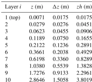
Table 2.Nodal depth,z, thickness,1z, and depth at the layer inter-face,zh, of the 10 soil layers used by CLM.

Layeri z(m) 1z(m) zh(m) 1 (top) 0.0071 0.0175 0.0175 2 0.0279 0.0276 0.0451 3 0.0623 0.0455 0.0906 4 0.1189 0.0750 0.1655 5 0.2122 0.1236 0.2891 6 0.3661 0.2038 0.4929 7 0.6198 0.3360 0.8289 8 1.0380 0.5539 1.3828 9 1.7276 0.9133 2.2961 10 2.8646 1.5058 3.8019

values of the resampled particles using the vector of normal-ized importance weights.

The measurement errors of the soil moisture observations are assumed to be zero-mean Gaussian with standard devi-ation,σ =0.02 m3m−3. This results inR=4×10−4Im in

Eqs. (4) and (17), respectively. We admit that 0.02 m3m−3is clearly larger than the uncertainty of the mean soil moisture content averaged over the 41 values. A larger observation er-ror alleviates potential problems with filter inbreeding. Also, we account crudely for errors in LSM model formulation via parameter uncertainty and the use of a stochastic description of the precipitation record of the Rollesbroich site (discussed next). In other words, thek×1 process noise vector,wt, in

Eq. (2) consists of zeros. However, we agree that it can be expected that we have other model structural errors, for ex-ample in relation to the representation of photosynthesis.

The hyetograph of each ensemble member is derived by multiplying the measured hourly precipitation rates of the tipping bucket by multipliers drawn from a unit-mean nor-mal distribution with a standard deviation of 0.10. This is equivalent to a heteroscedastic error of 10 % of the observed precipitation (Hodgkinson et al., 2004). Forcing variables which govern evapotranspiration (incoming shortwave and longwave radiation, air temperature, relative humidity, and wind speed) were not corrupted.

The initial values of VIC-3L and CLM parameters are sampled at random using a simple two-step procedure. This approach honours soil textural data and is consistent with related results published in the literature. First, we drawN

times from each marginal distribution listed in Table 1 un-der the column “perturbation”. These distributions originate from Han et al. (2014) for CLM, and Demaria et al. (2007) and Troy et al. (2008) in the case of VIC-3L. This results in a

N×dmatrix of perturbations for VIC-3L and CLM, respec-tively. We then create the initialN×d parameter ensemble of VIC-3L and CLM by adding each perturbation matrix to a deterministic vector of “best-guess” parameter values for each model. This initial parameter ensemble is the same for all the assimilation methods. For CLM, this best-guess

vec-tor is simply equivalent to the areal-averaged sand, clay, and organic matter fraction of each of the 10 soil layers, respec-tively. In the case of VIC-3L, we guess thatβ=15 (all lay-ers),b=0.2, andDm=13 (mm d−1), and derive the value of log10ks(log10(m s−1)) of all three soil layers from the mea-sured mean areal sand fraction at each of those depths. The best-guess parameter values of VIC-3L and CLM and their respective marginal distributions are jointly also referred to hereafter asprior parameter distribution. We want to com-pare EnKF and PF starting from the same prior distribution in order to make a more meaningful comparison. EnKF as-sumes a Gaussian distribution, but the PF not. We believe that assuming an initial uniform distribution is a neutral as-sumption good for comparing EnKF and PF.

One may debate our best-guess parameter values of VIC-3L and CLM and their respective marginal distributions. Nevertheless, the prior parameter distribution used herein in-troduces more than sufficient dispersion into the best-guess parameter values to rapidly overcome a possibly deficient ini-tial model parameterization. Note that the prior uncertainty of the two texture parameters (sand and clay fraction) in CLM is much larger than their spread derived from the tex-ture measurements of each soil layer. This inflation of the prior distribution is done purposely to account indirectly for the epistemic uncertainty of the pedotransfer functions that are used to predict the soil hydraulic parameters. Indeed, the prior parameter uncertainty of the sand and clay fraction should be large enough to guarantee a sufficient soil mois-ture spread of the ensemble, which is of crucial importance for an adequate performance of the different data assimila-tion methods.

Figure 2 shows the measured records of daily precipitation and daily air temperature for the 10-month measurement pe-riod used herein. The measurement pepe-riod is rather wet, with several intensive precipitation events during the summer. For example, notice the event on 27 July 2012 in which 31 mm of precipitation fell in just 1 h. Our experience suggests that such extreme rainfall events corrupt the parameter estimates, in large part due to an inadequate description and/or char-acterization of surface runoff. What is more, the correlation between the hydraulic parameters of the different layers of our soil domain and the moisture state deteriorates rapidly close to saturation. Therefore, on days with rainfall in excess of 20 mm we resort to state estimation only, and proceed with this the next 2 consecutive days to give VIC-3 and CLM suf-ficient opportunity to remove, via desuf-ficient surface transport or state updating, the excess water. On the third day after each 20 mm+precipitation event, we resume joint LSM state and parameter estimation.

Figure 2.Historical records of daily mean air temperature (solid black line; lefty-axis) and precipitation (blue bars; righty-axis) in the period from 1 March to 31 December 2012 for the Rollesbroich experimental test site in the Eifel mountain range in western Germany. The grey region demarcates the 5-month assimilation period (1 March to 31 July 2012) which is used for VIC-3L and CLM calibration using joint parameter and state estimation. The subsequent 5-month period between 1 August and 31 December 2012 serves as our evaluation period to verify the performance of the calibrated VIC-3L and CLM models without state estimation.

1. Open-loop simulation. We evaluate the LSMs from 1 March 2012 to 31 December 2012 with time-invariant parameters via Monte Carlo simulation using a large number of draws from the prior parameter distribution summarized in Table 1 and Sect. 4.2.

2. State updating with EnKF. The soil moisture state vari-ables were updated during the 5-month calibration pe-riod using the SPADE moisture content measurements. In theory, soil moisture assimilation should improve our estimates of the initial states of the evaluation pe-riod. We posit that this enhanced state-value character-ization should improve the accuracy of the LSM sim-ulated (predicted) soil moisture values during the first few days/weeks of the evaluation period, after which the model performance deteriorates rapidly over time in the absence of recursive state adjustments.

3. Joint state-parameter estimation using RRPF, PMCMC, and EnKF with state augmentation and dual estimation. The soil moisture state variables and model parameters are estimated during the 5-month calibration period us-ing the SPADE soil moisture measurements. The pa-rameter values and state variables at the end of the cali-bration data period are used for the evaluation period.

4.3 Summary statistics

We used the Nash–Sutcliffe model efficiency (NSE) and the root mean square error (RMSE) to evaluate the quality-of-fit of VIC-3L and CLM predicted (simulated) soil moisture val-ues during the calibration (assimilation) and evaluation

pe-Table 3.Summary of the different numerical experiments used in this paper for CLM and VIC-3L and their respective abbreviations used in the subsequent tables and figures.

Scenario description Abbreviation

Open-loop simulation OpenLoop EnKF with state estimation noParamUpdate EnKF with state augmentation EnKF-AUG EnKF with dual estimation EnKF-DUAL RRPF with ad hoc parameter perturbations RRPF

PMCMC PMCMC

riods. These two metrics are computed separately for the 5, 20, and 50 cm measurement depths as follows:

NSEi=1−

Pn

t=1 eyi,t−yi,t 2

Pn t=1

eyi,t−

1

n

Pn t=1eyi,t

2,

RMSEi =

r 1

n

Xn

t=1eyi,t−yi,t 2

, (24)

where_ey_i,t andy_i,t denote the measured and ensemble mean predicted soil moisture contents at timet, the subscripti con-stitutes an index for measurement depth,i= {1, . . .,3}, and

the soil moisture observations were the only data available to evaluate the results of VIC-3L and CLM and each data assimilation method.

5 Results

In this section we present the results of our numerical exper-iments. We first discuss our findings for VIC-3L followed by the results of CLM. Sect. 6 proceeds with a discussion of the main findings.

5.1 VIC-3L

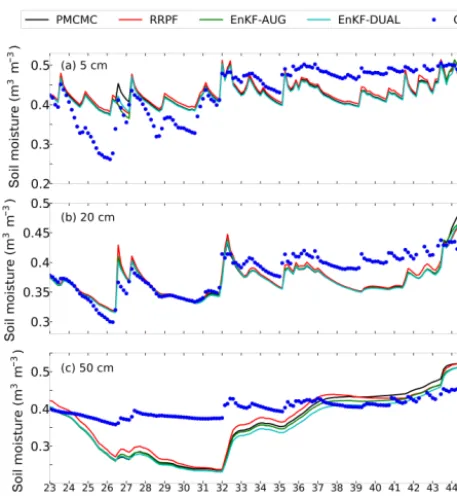
Figure 3 displays the observed (blue dots) and VIC-3L pre-dicted soil moisture values (solid lines) at (a) 5, (b) 20, and (c) 50 cm depths using PMCMC (black), RRPF (red), EnKF-AUG (green), and EnKF-DUAL (cyan). As the Rollesbroich test site experiences a yearly average precipitation of more than about 1000 mm it is not surprise that the upper soil layer at 5 cm is rather wet with volumetric soil moisture contents that vary dynamically between 0.3 and 0.5 cm3cm−3in re-sponse to atmospheric forcing. This is especially true during the summer months (weeks 12–22) and explained by a rapid succession of rainfall and drying events. The larger poros-ity values of the surface layer explain the relatively high soil moisture contents of the 5 cm measurement depth. The stor-age time series of the deeper soil layers at 20 and 50 cm depths exhibit a rather negligible temporal variation with soil moisture values that range between 0.3 and 0.4 cm3cm−3 and show a damped and lagged response to rainfall. Note that the soil water storage of the deepest layer increases steadily during the year. This implies a drainage flux from the top soil to the aquifer (and drainage channels).

The different data assimilation methods demonstrate a rather similar performance with VIC-3L predicted moisture contents that track reasonably well the three different layers. Note however that RRPF does not reproduce well the mea-sured data at 50 cm depth in the period from March (week 1) to June (week 17). This might be caused by filter inbreeding of the states, and will be discussed later (see also Fig. 9b). Nevertheless, RRPF recovers the observed soil moisture data in week 18. Although difficult to see, the EnKF produces the best results at 50 cm depth (state augmentation and dual esti-mation).

Table 4 summarizes the NSE and RMSE values of PM-CMC, RRPF, EnKF-DUAL, and EnKF-AUG for the cali-bration (assimilation) period. We also list the performance of VIC-3L without data assimilation (OpenLoop) using the mean soil moisture time series of many different realiza-tions of the prior parameter distribution, and include RMSE and NSE values of the EnKF for state estimation only (noParamUpdate) using VIC-3L parameterizations drawn randomly from its prior parameter distribution. The open loop deviates most from the measured values, with RMSE

Figure 3.Assimilation period: observed (blue dots) and VIC-3L predicted time series (solid lines) of soil moisture content at depths of(a)5,(b)20, and(c)50 cm in the Rollesbroich site. Color cod-ing is used to differentiate between the results of PMCMC (black), RRPF (red), EnKF-AUG (green), and EnKF-DUAL (cyan). The first days of weeks 1 and 22 are 1 March 2012 and 26 July 2012, respectively.

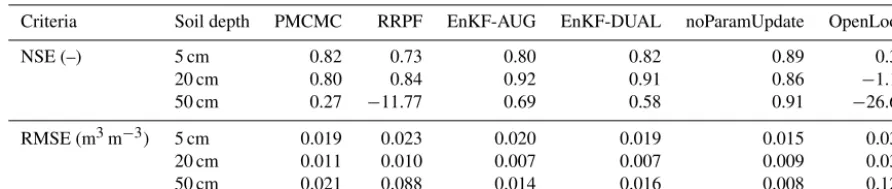
mea-Table 4.Calibration period: values of the NSE and RMSE summary statistics of the quality-of-fit of VIC-3L for the Rollesbroich soil moisture observations at 5, 20, and 50 cm depths using the PMCMC, RRPF, EnKF-AUG, and EnKF-DUAL data assimilation methods. For completeness, we also list the performance of the EnKF for state estimation only (noParamUpdate) using VIC-3L parameter values drawn randomly from the prior parameter distribution, and the performance of an open-loop run of VIC-3L (OpenLoop) using the mean simulation of many different VIC-3L parameterizations drawn randomly from the prior parameter distribution (see Table 1 and Sect. 4.2).

Criteria Soil depth PMCMC RRPF EnKF-AUG EnKF-DUAL noParamUpdate OpenLoop NSE (–) 5 cm 0.82 0.73 0.80 0.82 0.89 0.33 20 cm 0.80 0.84 0.92 0.91 0.86 −1.16 50 cm 0.27 −11.77 0.69 0.58 0.91 −26.65 RMSE (m3m−3) 5 cm 0.019 0.023 0.020 0.019 0.015 0.036 20 cm 0.011 0.010 0.007 0.007 0.009 0.037 50 cm 0.021 0.088 0.014 0.016 0.008 0.129

surement layer, and PMCMC exhibits a better performance than RRPF.

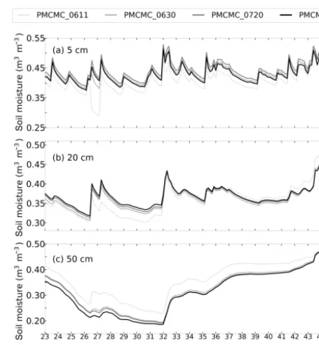
Figure 4 presents trace plots of VIC-3L parameters during the 5-month calibration period using the PMCMC (black), PF (red), EnKF-AUG (green), and EnKF-DUAL (cyan) data assimilation methods. We display the ensemble mean satu-rated hydraulic conductivity (log10ks in m s−1) at (a) 5 cm, (b) 20 cm, and (c) 50 cm depths, (d) b, β at (e) 5 cm, (f) 20 cm, and (g) 50 cm depths, and (h) the maximum base-flow velocityDmin mm day−1. In general, the different data assimilation methods result in somewhat similar trajectories of the ensemble mean parameter values during the calibration period. In particular, the parameter trace plots of EnKF-AUG and EnKF-DUAL appear almost identical, with the exception of parameterbandβat 50 cm depth. Note that the parameters of the surface layer exhibit the most dynamics in response to atmospheric forcing. PMCMC exhibits significant temporal dynamics. This is not surprising, and a consequence of the MCMC resampling step that is used to rejuvenate the pa-rameter samples (e.g., Vrugt et al., 2013). In the first place, the DREAM-type proposal distribution that is used to create candidate particles allows for relatively large moves in the parameter space. Second, only a small LSM trajectory be-tween two successive soil moisture observations is used to determine the acceptance probability of each candidate par-ticle. With such a short (re)-simulation period, insensitive pa-rameters are allowed to transition to very different values, as they do not affect the model output between the two obser-vations and thus the likelihood of a candidate particle. Alto-gether, this also contributes to a stronger dependency of PM-CMC on the initial parameter ensemble. This collection of parameter vectors is drawn randomly from the prior parame-ter distribution and differs per trial depending on the random seed. The use of a larger historical simulation period (going back further in time) would better constrain VIC-3L parame-ters but also increase significantly the computational burden of resampling. Nonetheless, the ensemble mean VIC-3L pa-rameter values of the different data assimilation methods are remarkably similar at the end of the calibration period,

af-ter assimilating the soil moisture observations of week 22. The exception to this is parameterb, whose trajectories dif-fer most, with values at the end of the calibration period that range between values of 0.11 for RRPF and 0.25 for EnKF-DUAL. Finally, parameterDm converges systematically to values of 1–2 mm day−1but at a different rate for the data assimilation methods. The EnKF-AUG, EnKF-DUAL, and PMCMC methods need just a few soil moisture observations to determine the value ofDm, whereas RRPF converges at a much slower pace. This might explain the rather inferior per-formance of RRPF for the 50 cm measurement depth during a substantial part of the assimilation period.

To provide a better understanding of the ensemble spread of VIC-3L parameters, please consider Fig. 5, which presents trace plots of the sampled log10ks(left column) andβ (right column) values at the 20 cm measurement depth for theN =

100 members. Results are presented in order of (a–b) PM-CMC (grey), (c–d) RRPF (red), (e–f) EnKF-AUG (green), and (g–h) EnKF-DUAL (cyan), and the ensemble mean is indicated with the solid black line. The ensemble members cover a relatively large part of the prior distribution of both parameters, with the exception of RRPF, which seems to un-derestimate the actual uncertainty of log10ks andβ. This is an artefact of smalls, which discourages large parameter ad-justments. Nevertheless, note that the ensemble mean of the parameters is rather unaffected by assimilation of the soil moisture data, except for the small increase in log10ks and

βin late April due to increased precipitation in the following months (see also Fig. 2).

ini-Figure 4.Trace plots (solid lines) of VIC-3L parameters. Saturated hydraulic conductivity (log10ks in m s−1) at(a)5 cm,(b)20 cm, and (c)50 cm depths,(d)b,βat(e)5 cm,(f)20 cm, and(g)50 cm depths, and(h)the maximum baseflow velocity,Dm, in mm day−1during the 5-month assimilation period. Color coding is used to differentiate between the results of PMCMC (black), RRPF (red), EnKF-AUG (green), and EnKF-DUAL (cyan). The first days of weeks 1 and 22 are 1 March and 26 July 2012, respectively.

Figure 5. Sampled trajectories of theN=100 ensemble members of the saturated hydraulic conductivity (log10ks in m s−1) at 20 cm

depth(a, c, e, g)and parameterβ(b, d, f, h)of VIC-3L during the 5-month assimilation period of weeks 1 to 22 using(a–b)PMCMC (grey)