Introducing a rainfall compound distribution model based on weather patterns sub sampling

doi:10.5194/hess-14-951-2010

© Author(s) 2010. CC Attribution 3.0 License.

Earth System

Sciences

Introducing a rainfall compound distribution model based on

weather patterns sub-sampling

F. Garavaglia1, J. Gailhard1, E. Paquet1, M. Lang2, R. Garc¸on1, and P. Bernardara3 1_{EDF – DTG, 21 Avenue de l’Europe, BP 41, 38040 Grenoble Cedex 9, France}

2_{HHLY, CEMAGREF, 3bis quai Chauveau, CP220, 69366 Lyon Cedex 09, France} 3_{EDF – R&D LNHE, 6 quai Watier, 78401 Chatou, France}

Received: 15 December 2009 – Published in Hydrol. Earth Syst. Sci. Discuss.: 15 January 2010 Revised: 1 May 2010 – Accepted: 1 June 2010 – Published: 16 June 2010

Abstract. This paper presents a probabilistic model for daily rainfall, using sub-sampling based on meteorological circu-lation. We classified eight typical but contrasted synoptic situations (weather patterns) for France and surrounding ar-eas, using a “bottom-up” approach, i.e. from the shape of the rain field to the synoptic situations described by geopotential fields. These weather patterns (WP) provide a discriminat-ing variable that is consistent with French climatology, and allows seasonal rainfall records to be split into more homo-geneous sub-samples, in term of meteorological genesis.

First results show how the combination of seasonal and WP sub-sampling strongly influences the identification of the asymptotic behaviour of rainfall probabilistic models. Fur-thermore, with this level of stratification, an asymptotic ex-ponential behaviour of each sub-sample appears as a reason-able hypothesis. This first part is illustrated with two daily rainfall records from SE of France.

The distribution of the multi-exponential weather patterns (MEWP) is then defined as the composition, for a given sea-son, of all WP sub-sample marginal distributions, weighted by the relative frequency of occurrence of each WP. This model is finally compared to Exponential and Generalized Pareto distributions, showing good features in terms of ro-bustness and accuracy. These final statistical results are com-puted from a wide dataset of 478 rainfall chronicles spread on the southern half of France. All these data cover the 1953– 2005 period.

Correspondence to: F. Garavaglia ([email protected])

1 Introduction

EDF ( ´Electricit´e de France) design floods of dam spill-ways are now computed using a stochastic method named SCHADEX (Climatic-hydrological simulation of extreme floods) (Paquet et al., 2006). This method aims at estimating extreme flood quantiles by the combination of a rainfall prob-abilistic model and a continuous conceptual rainfall-runoff model (see Boughton and Droop, 2003 for a review). The purpose of this paper is to introduce the rainfall probabilistic model used in the SCHADEX method, based on a weather patterns sub-sampling. After introducing the weather pat-terns classification, we will first discuss the impact of this additional sub-sampling level on the identification of asymp-totic behaviour of rainfall probabilistic models. We will fi-nally present the formulation and the properties of this model and compare it with standard models.

the basis of point data (Koutsoyiannis, 2004). Regional ap-proaches, by gathering data at a spatial scale, allow to im-prove the robustness of parameter estimation. It consists ei-ther in refining the analysis to homogeneous climatic zones, in which the shape parameter is considered to be constant (Madsen et al., 1995; Ribatet et al., 2007; Pujol et al., 2008), or in using indirect methods, i.e. methods based on stochas-tic simulation of rainfall events, such as the SHYPRE method (Arnaud et al., 2007), in which the parameters are estimated using a regional approach (SHYREG method, Arnaud et al., 2006a).

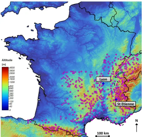
In order to improve robustness without loosing accuracy in extreme rainfall estimation, we propose an alternative ap-proach using a classification of atmospheric circulation pat-terns. These weather patterns (WP) provide a discriminating variable that is consistent with French climatology, and allow seasonal rainfall records to be split into more homogeneous sub-samples, in term of meteorological genesis. An expo-nential POT model is used to fit the distribution of each sub-sample. The distribution of the multi-exponential weather patterns (MEWP) is then defined as the composition, for a given season, of all WP sub-sample marginal distributions, weighted by the relative frequency of occurrence of each WP. The weather pattern classification, so-called EDF 2006, is described in Sect. 2 below. The need for seasonal and weather pattern sub-sampling is explained in Sect. 3. In Sect. 4 we discuss the effect of sub-sampling on the identi-fication of the asymptotic behaviour of rainfall probabilistic models. Section 3 and Sect. 4 are illustrated with the daily rainfall records from Lyon and St Etienne en D´evoluy (SE France). In Sect. 5 the MEWP rainfall probabilistic model is introduced. In order to assess the robustness and the ac-curacy of the proposed model, more global statistical results are computed from a wide dataset of 478 rainfall chronicles spread on the southern half of France (Fig. 1). All these data cover the 1953–2005 period.

2 Weather patterns classification

2.1 Context

The relationship between large-scale atmospheric circulation and precipitation events has been studied for a long time (see Yarnal et al., 2001; Bo´e et al., 2008; Martinez et al., 2008, for a review), especially over Western Europe, and it has been demonstrated that analysing synoptic situation can provide significant information on heavy rainfall events (Littmann, 2000).Various authors focused on the Mediterranean area (Romero et al., 1999; Littmann, 2000; Martinez et al., 2008). From this point of view, a classification based on a lim-ited number of typical but contrasted synoptic situations (or weather patterns) is a useful tool to link rainfall events with its generating processes. In this section, we identify the

Fig. 1. Localisation of the 478 rain gauges used in this study (Lyon

and St Etienne en D´evoluy rain gauges are highlighted).

weather patterns for France and the resulting classification of rainy days.

To define a daily synoptic situation over France and sur-rounding areas, we used a dataset that has already been op-timised in previous works on quantitative precipitation fore-cast using the analogue method (Guilbaud et al., 1998; Obled et al., 2002):

– Geopotential height fields at 700 and 1000 hPa pressure levels, at 0 h and 24 h, defined on 110 grid points; – Analysis centred on south-eastern France from 6.2◦W

to 12.9◦_{E, and from 38.0}◦_{N to 50.3}◦_N.

In this way, each day can be defined in the<440 mathe-matical space of the geopotential fields concerned (four fields defined on 110 points).

2.2 A “bottom-up” approach for the identification of weather patterns

In our classification process, “bottom-up” should be under-stood as firstly identifying the centroids of classes using our variable of interest (i.e. rainfall), and secondly projecting them into the<440space of geopotential heights.

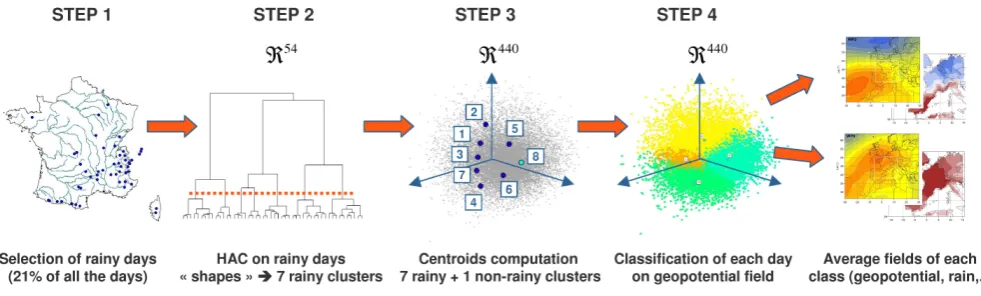
The whole classification process is summarized in Fig. 2, and consists of the following steps:

Fig. 2. WP classification flowchart.

average rain depth (computed on the 54 chronicles) ex-ceeding 5 mm, are considered as rainy days. We then normalize each local rain depth by the average precipi-tation of the day concerned, as a way of considering the “shape” of the rain field rather than its scale. Instead than using thehow much does it rain information, we use thewhere does it raininformation in our process. – STEP 2. A Hierarchical Ascendant Classification

(HAC) is then performed on this population of rainy day shapes, as defined in a<54space. The dendrogram of this HAC showed that seven rainy classes could be cho-sen, at this stage the remaining days (79% of days) are combined in a non-rainy class.

– STEP 3. During this step the centres of gravity (or cen-troids) of the eight classes are calculated in the<440 space of geopotential heights.

– STEP 4. Each day of the 1953–2005 period is attributed to the weather pattern (WP) whose centroid is the clos-est in the<440, using the Teweles-Wobus score (Tewe-les and Wobus, 1954) as measure of proximity between synoptic situations. This led to changes for some days in the period 1956–1996 that were already classified by the HAC of rain, specially WP8 days (see below for the def-inition of WP8). Note that the Teweles-Wobus distance is used because we want to focus on atmospheric cir-culation, whatever the mean height of the geopotential fields (we could also have used other distances e.g. cor-relation between fields).

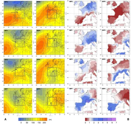
The obtained WPs are illustrated in Fig. 3a by their mean 1000 hPa geopotential field at 0 h. For pedagogical reasons, the fields are presented in logical order in terms of atmo-spheric circulations, i.e. 2-1-3-7-4-6-5 and 8 (see Fig. 2 Step 3). For each WP (except for WP8) an arrow indicates the at-mospheric flow of low layers induced by the average synoptic fields. The size and the direction of the arrow are a qualitative indication of the strength and direction of the wind. Fig. 3b

shows the corresponding relative precipitation fields (ratio of WP mean to “all day ” mean precipitation) over western Europe. For this purpose, we used a gridded version of the European Climate Assessment and Data (ECA&D) of mean daily precipitation (Haylock et al., 2008). The grid resolution is 0.5×0.5◦and the data cover the period 1953 to 2005.

These patterns give a picture of the diversity of rainy syn-optic situations over France. They were named in relation with the atmospheric circulation they favour. WP2 (Steady Oceanic), WP1 (Atlantic Wave) and WP3 (South-West Cir-culation) correspond to westerly oceanic circulations, WP1 being the most rainy pattern over the study area. WP7 (Cen-tral Depression) and WP4 (South Circulation) correspond to Mediterranean circulations, which bring heavy rains to south-eastern France. WP6 (East Return) also corresponds to a Mediterranean circulation, but rain is generally limited to the Italian border and eastern Pyrenees. WP5 (North East) is a continental circulation, and finally WP8 (Anticyclonic) shows no well-defined circulation, as expected for a non-rainy day. The occurrence statistics of the eight WPs are presented in Table 1. For the whole year, the most frequent WP is the Anticyclonic one (WP8), followed by the Steady Oceanic (WP2) and the South Circulation (WP4). However, these figures change with the season, for example WP2 is more frequent in winter, and WP8 in summer.

2.3 Suitability of the proposed WP classification

Fig. 3. Average geopotential height at 1000 hPa of the eight WP (A) and the ratio of the mean WP to global mean precipitation (B). The

frame highlights the area of interest (from 6.2◦W to 12.9◦E, and from 38.0◦N to 50.3◦N) and the arrows indicate the atmospheric flow of low layers.

Table 1. Yearly and seasonal statistics of occurrence for the eight WP (records for the period 1953–2005).

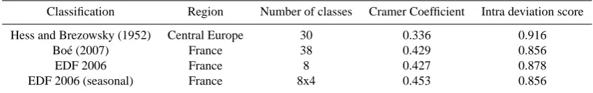
Table 2. Comparison of the discriminating power of three classifications (average of statistics made on 54 rainfall records).

Classification Region Number of classes Cramer Coefficient Intra deviation score Hess and Brezowsky (1952) Central Europe 30 0.336 0.916

Bo´e (2007) France 38 0.429 0.856

EDF 2006 France 8 0.427 0.878

EDF 2006 (seasonal) France 8x4 0.453 0.856

evaluated on its ability to propose a reasonable typology of the phenomenon concerned.

Two other available classifications were evaluated and compared to the one proposed here: the well-known Hess-Brezowsky classification (Hess and Hess-Brezowsky, 1952), be-cause it is often used for comparison, and another French classification (Bo´e, 2007), which is also used for precipita-tion analysis. The latter classificaprecipita-tion in fact comprises four classifications of 8–10 classes, one for each season (DJF, MAM, JJA, SON). The discriminating power of the three classifications was checked for rain/no rain occurrence, us-ing appropriate criteria like the Cramer test (Bardossy et al., 1995). This coefficient ranges between 0 (no dependence be-tween the classification and the rain/no rain occurrence) and 1 (absolute dependence). Another criterion is also computed to check how the classification minimizes deviation within classes. The chosen criterion is the ratio of intra classes de-viation to total dede-viation. This coefficient ranges between 1 (equal deviation within classes than the total population) and 0 (no deviation within classes : each class contains the same numeric value). These criteria are first computed on each of our 54 rainfall chronicles on the period 1953–1998 and then averaged to obtain a single value. The results of the com-parison are presented in Table 2, and show that the present classification based on the eight WPs has good discriminat-ing power for the rain occurrence and value.

In addition, the corresponding average rain fields are con-trasted (Fig. 3b). In our opinion, one of the major advantages of this classification is that it remains applicable throughout the year, enabling flexible use. For example, in a recent study by Gottardi (2009), this classification was used to interpolate daily precipitation fields over French mountainous regions. It is now time to evaluate its interest for heavy rainfall distri-bution.

3 Extreme value theory and sampling techniques

3.1 Sampling techniques for extreme values

The extreme value theory is based on the fundamental hy-pothesis that the random variable realizations (daily rain-fall in our study) are independent and identically distributed (i.i.d). Two standard sampling techniques are used to build samples coming closer to these hypotheses:

– Block Maximum (BM). The maximum values within blocks of equal length of data are selected. The choice of block size can be critical as too small blocks can lead to bias and too large blocks generate too few block maxima, thus giving a large estimation variance (Coles, 2001). Usually the one-year block is used for daily dis-charges or rainfall data, leading to the annual maxima (AM). According to Coles et al. (2003), asymptotic con-sideration suggest that the distribution of AM should be approximately a member of the generalized extreme value (GEV) distribution.

– Peaks over threshold (POT). All the events exceeding a given threshold are selected (see Lang et al., 1999; Rosbierg and Madsen, 2004, for a review). Once again according to Coles (2001), such a sample may be re-garded as independent realizations of a random variable whose distribution can be approximated by a member of generalized Pareto distribution.

Always according to Coles et al. (2003), if daily series are available, POT sampling is better that AM sampling, because additional information on several large events that occur dur-ing the same year is taken into account.

To ensure independence of POT values, an additional cri-terion based on a minimum time period between two suc-cessive events is usually applied. In this paper, we begin to introduce a new variable, called the “central rainfall”, which is, at a daily time step, rainfall exceeding 1 mm and greater than the quantity of rain on the preceding and following day. This CR sampling is closely linked to the rainfall-runoff sim-ulation process part of the SCHADEX method. The indepen-dence of this kind of re-sampled rainfall time series has been checked by computing the first order lag autocorrelation co-efficients for the whole dataset (map on Fig. 1). The median autocorrelation coefficient is 0 for AM sampling method, 0.07 for CR sampling method and 0.23 for daily time-series. We therefore selected POT values of “central rainfalls”. In the Lyon records, the so-called “central rainfalls” represent about 17% of all daily rainfall (63% of the days being non-rainy days, and the 20% remaining days thus having less rain-fall than the preceding or following days).

illustrated by considering daily discharges of small moun-tain catchments where high values are commonly observed either in spring or autumn. In this case, two populations linked to very different hydrological processes (snowmelt or heavy rain runoff floods) are mixed by BM or POT sam-pling (Hirschboeck et al., 1987; Petrow et al., 2007), making the “identically distributed” hypothesis harder to ensure, and consequently the use of extreme value statistical theory more questionable.

Therefore, two complementary sub-sampling techniques for rainfall records are introduced here to more closely ap-proach the i.i.d. hypothesis.

3.2 Seasonal sub-sampling

In most places in the world and in a wide range of climates, rainfall displays strong seasonal variability. At a given lo-cation, the frequency and intensity of rainfall is driven by the meteorological situation, whose genesis is strongly influ-enced by large scale seasonal factors, for example variation in solar input (incidence of sunlight, day length), sea sur-face temperatures, the position of long lasting high or low pressure centers etc. The factors that cause heavy rainfall events are numerous, various and complex, and they inter-act at different scales, but their seasonal variation pattern has a true climatological consistency. This is common sense in strong bipolar precipitation regimes (like monsoon), but is also true in temperate climates with more mixed influences. For example, heavy rains hitting the French, Spanish and Ital-ian regions surrounding the Mediterranean Sea most likely occur during fall (September to November). This kind of pattern must be taken into account by appropriate seasonal sampling to produce more homogeneous sub-populations for heavy rainfall analysis (Lang and Desurosne, 1994; Djerboua and Lang, 2007). In extreme rainfall studies for France, we usually consider two to four non-overlapping seasons.

Fig. 4 is a box plot of annual daily rainfall maxima for each month at Lyon and St Etienne en D´evoluy. The sea-sonal pattern is rather common for daily rainfall in southern France, with the highest quantiles (“season-at-risk”) occur-ring between September and November (as shown for St Eti-enne en D´evoluy). For Lyon, this “season-at-risk” is more likely June to November.

3.3 Weather Pattern based sub-sampling

As indicated in Sect. 2.1, in Europe, the links between atmo-spheric circulation patterns and heavy rainfall events have been widely studied in various locations. The analysis do-main on which the classification is built is generally wide (several degrees of latitude and longitude), and thus has a re-gional sense. A discrimination of rainfall records based on such a classification is one way to gather observations ac-cording to similar generating meteorological processes, and hence progress toward to the homogeneity of sub-samples.

One application was described by Ramos et al. (2001) for the 30’ rainfall in Marseilles (France), showing two distinct asymptotic behaviours depending on the presence of a meso-scale convective system. This approach can also provide ad-ditional information about extreme rainfall events, thus en-hancing probabilistic analysis (Klemeˆs, 1993). Figure 5 is a box-plot of annual maxima for each weather pattern for Lyon and St Etienne en D´evoluy. The WP4 (South Circula-tion), WP7 (Central Depression), and to a lesser extent WP1 (Atlantic Wave), clearly have higher quantiles than the other weather patterns. We will now show how to integrate these sub-samplings into rainfall probabilistic models.

4 Taking into account seasonal and weather pattern sub-sampling

4.1 Global formulation

LetY represents the hydrologic variable of interest such as daily rainfall (or central rainfall, see above). Let us now con-sider a range of seasonsi=1,...,S, whereSis the number of seasons that allows appropriate seasonal division of the local precipitation regime (Sequal to 2 or 4 generally in France).

Let us also consider a range of weather patternsj=1,..., NWP, where NWP is the number of weather patterns that provides a robust discrimination of the meteorological situa-tions of the study region (for France, NWP equal to 8 for the classification presented in Sect. 2).

To build sub-samples based on seasons and weather pat-terns, the hydrologic variableY is partitioned intoS·NWP variables,Y_NWPS=i_=j, with respect to seasons and weather pat-terns, as follows:

Y=

S

[

i=1

Yi andYi= NWP

[

j=1

Y_ji (1)

As mentioned before, asymptotic behaviour of POT values of a daily rainfall sub-sample of seasoniand WPj, may be approached by a GP distribution, which takes the form:

F_ji(z)=PrhZ_ji =Y_ji−ui_j< zi=1− 1+ξ_ji z λi_j

!−1

ξ i j

(2)

with a parameter space nλi_j,ξ_ji:λi_j>0,ξ_ji∈ <o, and a thresholdui_j.

As the set of seasonal POT values across all WP is the union of the POT values within each WP, the seasonal rainfall distribution is computed from a mixture distribution of GP distribution for each WP. This seasonal distribution takes the form:

Fi(z)= NWP

X

j=1

Fig. 4. Box plot of the annual maxima for each month at Lyon rain gauge (left) and St Etienne en D´evoluy (right) (records for the period

1953–2005). Dashed lines and double arrow highlight the “season-at-risk” (season of occurrence of highest rainfall quantiles) at Lyon (June to November) and St Etienne en D´evoluy (September to November).

Fig. 5. Box plot of the annual maxima for each weather pattern at Lyon rain gauge (left) and St Etienne en D´evouly (right) (records for the

period 1953–2005). Dashed lines and double arrow highlight the “WPs-at-risk” (WP associated to highest rainfall quantiles): WP 7 and WP 4.

where weightp_ji is the relative occurrence of each WP within seasoni. The global distribution is therefore computed from a mixture distribution of each seasonal distribution, which takes the form:

F (z)=

S

X

i=1

Fi(z)·pi (4)

where weightpiis the relative occurrence of each season that is equal to the ratio of the number of events in the season to the total number of events.

4.2 Relation between sub-sampling and asymptotic behaviour

An appropriate tool for the threshold selection is the Mean Residual Life (MRL) plot, expressed as follow :

" u, 1

nu nu

X

i=1 (xi−u)

!

:u < xmax #

(5) wherex1,...,xnu consist of thenu observations that exceed

thresholdu, andxmaxis the largest of thexi. According to

Fig. 6. MRL plot for all year (A and D), “season-at-risk” (B and E) and WP 4 days within “season-at-risk” (C and F) at Lyon rain gauge (A,

B and C) and St Etienne en D´evoluy (D, E and F). Gray lines represent the 95% confidence interval. The dashed lines highlight the fitted value of the scale parameter according to an exponential model.

More specifically, the mean excess above the thresholdu0 should be constant, equal to the scale parameter λ for the case of exponential distribution (ξ=0), and should increase linearly with the threshold value for the Pareto distribution (ξ >0) (Shanbhag 1970). Confidence intervals, based on the hypothesis of normality of the sample means, can be added to the plot.

The graphical interpretation of an MRL plot may appear as subjective. However, in our study, it has been used to illustrate how the vision of the asymptotic behaviour of a given population may be dependent of the chosen sampling level (global, season, season and WP). Figure 6 shows MRL plots for the whole year, the “season-at-risk”, and for the WP4 days within the “season-at-risk”, at Lyon and St enne en D´evoluy rain gauges. Considering Fig. 6d (St Eti-enne en D´evoluy , global sample), a reasonable interpreta-tion of the increasing linear trend of the MRL plot may be a Pareto asymptotic underlying behaviour. This is more ques-tionable for the Fig. 6e (St Etienne en D´evoluy, “season-at-risk”), where asymptotic exponential behaviour could be a possible interpretation (22.6 mm/24 h scale parameter). The exponential hypothesis (36.9 mm/24 h scale parameter) be-comes a more natural choice for the Fig. 6f (St Etienne en D´evoluy, WP4 days within the “season-at-risk”). Similar conclusions can be drawn for the example of Lyon (Fig. 6a to

6c), but with an asymptotic exponential behaviour almost no-ticeable on the whole year MRL plot above 25 mm threshold (Fig. 6a).

The MRL plot is supposed to help to determine the asymp-totic behaviour of the underlying distribution, but we see how far the final diagnostic can depend on the chosen sub-sampling. In other words, the asymptotic behaviour might be exponential, but a standard sub-sampling (e.g. records from whole year or whole season) might completely mask it. Fur-thermore, under the hypothesis of an exponential asymptotic behaviour, a standard sub-sampling might lead to an underes-timation of the scale parameter: Lyon scale parameter rising from 13.9 mm/24 h (“season-at-risk”) to 18.3 mm/24 h (WP4 in “season-at-risk”), St Etienne en D´evoluy scale parameter from 22.6 mm/24 h to 36.9 mm/24 h. Figure 7 shows addi-tional MRL plots for Lyon WP7, WP6 and WP1 sub-samples (within “season-at-risk”) with a more apparent asymptotic exponential behaviour.

Fig. 7. MRL plot for WP7 (A), WP6 (B) and WP1 (C) days in the season from June to November (“season-at-risk”) at Lyon rain gauge. Gray

lines represent the 95% confidence interval. The dashed line highlights the fitted value of the scale parameter according to an exponential model.

5 Multi-exponential weather pattern distribution

5.1 Model formulation

Considering that the shape parameterξ_ji is equal to zero, the seasonal distribution given in Eq. 3 takes the form:

Fi(z)=

N W P

X

j=1

F_ji(z)·p_ji=

N W P

X

j=1

1−exp −z λi_j

!!

·p_ji (6)

This seasonal distribution is then named multi-exponential weather pattern (MEWP) distribution. To provide a continu-ous probabilistic description of the whole range of observed rainfall, the CDF of each sub-sample is extended below its thresholdui_j by a linear interpolation of empirical quantiles. Otherwise, the MEWP distribution would only be defined above the greatest threshold of all sub-samples.

In practice, selecting a threshold levelui_j is not an easy task. In order to avoid compromising the asymptotic charac-teristic of the fitted values - threshold too low - and to avoid enlarging the variance of the estimators - threshold too high -,ui_j was chosen equal to the 70% empirical quantile of each WP sub-sample. This choice of threshold was checked on MRL plots. It proved to be a good compromise for the dataset presented in Fig. 1.

The confidence intervals are computed using the bootstrap non-parametric method (Efron , 1979). It consists in a ran-dom extraction with replace of values from the actual sample (WP sampling), in order to produce new samples (Bootstrap samples) of the same dimension of actual one. For every Bootstrap samples, the quantiles of given frequencyf,qf,

are determined via the probabilistic model considered. If qB,α/2,qB,1−α/2are the empirical quantiles of frequencyα/2 and 1−α/2 of the empirical distributionqf, the confidence

interval at 1−α level is equal to

qB,α/2,qB,1−α/2around the quantile. In order to take into account the variability of the occurrence of each WP in the computation of bootstrap interval of confidence, we modeled this occurrence with a

Poisson law. So for every bootstrap simulation, we extract randomly from a Poisson law the occurrence of the WPs.

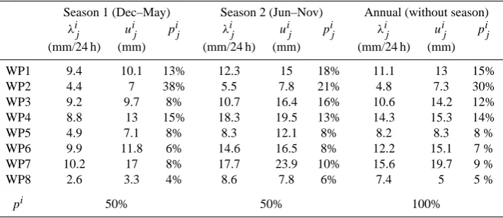
Table 3 shows the scale parameterλi_j, the threshold ui_j (corresponding to the 70% empirical quantile) and the weight p_ji of each WP within the annual and the two seasonal MEWP distributions (December to May, June to November) for the Lyon rain gauge. The last line gives the weightpi of each season used to compute the annual MEWP distribu-tion. These results reveal significant variability of the scale parameter in relation with the WP and the season. We con-sider this variability as an indication of the suitability of WP sampling: inappropriate sub-sampling would have produced randomly parsed samples of the whole record, with a rather uniform scale parameter for each sub-sample. Figure 8 il-lustrates the eight WP exponential distributions fitted on the Lyon rainfall records within the season Jun-Nov and the pe-riod 1953–2005. The x-axis of these graphs shows the return level, T (z), expressed in years, obtained from the density functionF (z), through the following expression:

T (z)= 1 1−F (z)Nn

(7)

Table 3. Scale parameterλi_j, thresholdui_j, weightpi_j for each weather pattern of the two seasonal MEWP distributions (season 1 from December to May and season 2 from June to November) for Lyon. Last columns detail the annual MEWP distribution (without seasonal sub-sampling). The weightspi refer to the weights used to compute the global MEWP distribution, if season sampling is used.

Season 1 (Dec–May) Season 2 (Jun–Nov) Annual (without season)

λi_j ui_j pi_j λi_j ui_j pi_j λi_j ui_j p_ji

(mm/24 h) (mm) (mm/24 h) (mm) (mm/24 h) (mm) WP1 9.4 10.1 13% 12.3 15 18% 11.1 13 15% WP2 4.4 7 38% 5.5 7.8 21% 4.8 7.3 30% WP3 9.2 9.7 8% 10.7 16.4 16% 10.6 14.2 12% WP4 8.8 13 15% 18.3 19.5 13% 14.3 15.3 14% WP5 4.9 7.1 8% 8.3 12.1 8% 8.2 8.3 8 % WP6 9.9 11.8 6% 14.6 16.5 8% 12.2 15.1 7 % WP7 10.2 17 8% 17.7 23.9 10% 15.6 19.7 9 % WP8 2.6 3.3 4% 8.6 7.8 6% 7.4 5 5 %

pi 50% 50% 100%

variability, but at a lower level. Choice of seasons may ap-pear as subjective but remains a mandatory step accounting for additional meteorological factors. For instance, concern-ing Mediterranean regions, the seasonal variation of heavy precipitations of a given WP is partly linked to the evolution of the Mediterranean Sea surface temperature. The eight WP exponential distributions illustrated in Fig. 8 are combined in a seasonal MEWP distribution (Fig. 9a) using the weightp_ji given in Table 3. Similarly the two seasonal MEWP distri-butions are combined in the global MEWP distribution illus-trated in Fig. 9b, according to the seasonal weightpi given in Table 3.

5.2 Model properties

Two important features of this model should be underlined: – A significant bend of the CDF for low to moderate

re-turn times can be represented, meaning non-exponential behaviour of distributions in the range of observable fre-quencies can be accounted for;

– For high and extreme quantiles (currently over 50 years of return period), the asymptotic behaviour becomes ex-ponential, and is fully parameterized by the scale pa-rameter and the relative frequencypi_j of the “WP-at-risk” and the “season-at-“WP-at-risk”.

However, the high flexibility of a probabilistic model, i.e. its ability to fit the largest observed values, often has the seri-ous drawback of lacking robustness for estimations of ex-treme quantiles. Figure 10 illustrates the robustness of the proposed probabilistic model. The MEWP distribution was compared with the Exponential (EXP) and GP distribution for the Lyon record. Both models were fitted locally (using maximum likelihood criterion) on two samples: the obser-vations of Jun–Nov season for the period 1953–2005, with

and without the maximum observed event (101 mm rainfall in 24 h on 30 September 1958).

Fig. 8. Exponential distributions of the eight WP sub-samples for Lyon rain gauges (data from the period 1953–2005; “season-at-risk” (June

to November)). The gray zone highlights the 90% confidence intervals.

accuracy test is not an easy task. Arnaud et al. (2006b) proposed a simple test, called “regional test”, assuming the spatial independence of highest quantiles. If n1 years of records are available for n2 rain gauges, the local estima-tion of the 1000 years return level by a correct probabilistic model, should be exceeded around(n1×n2)/1000 times on the whole dataset. This test is weakened by the spatial inde-pendence hypothesis, but it remains useful for model com-parison. It has been used on the 478 rain gauges dataset, for the 1953–2005 records on the “season-at-risk” (i.e. 25334 year×station), for the EXP, MEWP and GP models. Results are shown in Table 4 for the 1000 year return level. Theo-retically, the 0.999 quantile should be exceeded 25 times in this dataset. The EXP distribution underestimates it (60 ex-ceedances in the dataset), the GPD model overestimates it (7 exceedances), and the MEWP is closer to the theoretical value (32 exceedances). The MEWP distribution provides higher estimation of extreme rainfall, compared to the EXP distribution, correcting appropriately its notorious underesti-mating bias.

Table 4. Number of exceedances of the local millennial quantile

for the three models (EXP, MEWP, GPD) computed on the 478 rain gauges. Left columns shows the “theoretical” number of ex-ceedances expected.

f=0.999

“Theoretical” EXP MEWP GPD 25 60 32 7

6 Conclusions

The main features of the proposed MEWP approach can be summarized as follows:

– Construction of a rain-oriented weather pattern classifi-cation to approach the meteorological genesis of heavy rains, over an area of mixed climatological influences; – Discrimination of a rainfall record based on this

Fig. 9. MEWP distribution of the “season-at-risk” (June to November) (A) and global MEWP distribution (B) for the Lyon rain gauge (data

from the period 1953–2005). The gray zone highlights the 90% confidence intervals.

Fig. 10. Sensitivity of the extreme daily rainfall quantiles to the maximum value recorded by the Lyon rain gauge during the “season-at-risk” (June to November) for each model (EXP, MEWP and GP distribution).

– Use of marginal exponential distributions for each sub-sample based on a given weather pattern;

– Construction of a versatile compound distribution able to fit various shapes of empirical daily rainfall distri-butions up to the highest quantile observed, but with a simple and robust approach for asymptotic behaviour. An important concern was to approach the “i.i.d.” hy-pothesis of heavy rainfall samples. Independence of highest values is quite easy to ensure, but the homogeneity of sub-samples has to be checked indirectly:

– A priori, considering the discriminating power of the WP classification, it should be checked that the chosen classification minimizes deviation within classes, and maximizes it between classes;

– A posteriori, regarding the strong variability of rain-fall asymptotic behaviours induced by the WP sub-sampling.

Fig. 11.Relative deviation between two estimations of the100-years (left) and 1000-years (right) return levels.

For each model (EXP, MEWP and GP distribution) the two estimations are computed on the ”season-at-risk”,

with and without the observed maximum. The box plots show the spread of the results for the 478 rain gauges.

24

Fig. 11. Relative deviation between two estimations of the100-years (left) and 1000-years (right) return levels. For each model (EXP, MEWP

and GP distribution) the two estimations are computed on the “season-at-risk”, with and without the observed maximum. The box plots show the spread of the results for the 478 rain gauges.

quantiles. The proposed sampling method and the associated probabilistic model were presented and illustrated using the daily rainfall records for Lyon and St Etienne en D´evoluy. Some simple tests have been presented to assess the robust-ness and the accuracy of the proposed model. A more com-plete comprehensive statistical study of this approach, based on the introduced dataset of 478 rainfall time series, with a special focus on accuracy, will be presented in a future paper.

Acknowledgements. We acknowledge the E-OBS dataset from

the EU-FP6 project ENSEMBLES (http://www.ensembles-eu.org) and the data providers in the ECA&D project (http://eca.knmi.nl). We also thank the CERFACS team for providing the classification developped by J. Bo´e.

Edited by: H. Cloke

References

Arnaud, P., Lavabre, J., Sol, B., and Desouches, Ch.: R´egionalisation d’un g´en´erateur de pluies horaires sur la France m´etropolitaine pour la connaissance de l’al´ea pluviographique, Hydrolog. Sci. J., 53, 34–47, 2006a.

Arnaud, P., Lavabre, J., Sol, B., and Desouches, Ch.: Cartographie de l’alea pluviom´etrique de la France Colloque SHF: Valeurs rares et extrˆemes de d´ebit pour une meilleure maˆıtrise des risques, Lyon 15–16 March, 67–80, 2006b.

Arnaud, P., Fine, A., and Lavabre, J.: An hourly rainfall generation model applicable to all types of climate, Atmos. Res. 82, 230– 242, 2007.

Bardossy, A., Duckstein, L., and Bogardi, I.: Fuzzy rule-based clas-sification of atmospheric circulation patterns, Int. J. Climatol., 15, 1087–1097, 1995.

Bo´e, J.: Changement global et cycle hydrologique: une ´etude de r´egionalisation sur la France, PhD Thesis, University Paul Sabatier Toulouse III, Pp 256, Toulouse, 2007.

Bo´e, J. and Terray, L.: A weather type approach to analysing winter precipitation in France: twentieth century trends and influence of anthropogenic forcing, J. Climate, 21, 3118–3133, 2008. Boughton, W. and Droop, O.: Continuous simulation for design

flood estimation – a review, Environ. Modell. Softw., 18, 309– 318, 2003.

Coles, S.: An introduction to statistical modeling of extreme values, Springer, London, 2001.

Coles, S., Perricchi, L., and Sisson, S.: A fully probabilistic ap-proach to extreme rainfall modelling, J. Hydrol., 273, 35–50, 2003.

Djerboua, A. and Lang, M.: Scale parameter of maximal rainfall distribution: comparison of three sampling techniques, Revue des Sciences de l’Eau, 20, 111–125, 2007.

Efron, B.: Bootstrap methods: Another look at the jackknife, The Annals of Statistics?, 7, 1–26, 1979.

Gottardi, F.: Estimation statistique et r´eanalyse des pr´ecipitations en montagne, PhD Thesis, Polytechnic Institute of Grenoble, pp 252, Grenoble, 2009.

Guilbaud, S. and Obled, C.: Daily quantitative precipitation forecast by an analogue technique: optimisaion of the analogy criterion, C. R. Acad. Sci. Paris, Earth Planet. Sci., 327, 181–188, 1998. Haylock, M. R., Hofstra, N., Klein Tank, A. M. G., Klok,

E. J., Jones, P. D., and New, M.: A European daily high-resolution gridded data set of surface temperature and pre-cipitation for 1950-2006, J. Geophys. Res., 113, D20119, doi:10.1029/2008JD010201, 2008.

Hess, P. and Brezowsky, H.: Katalog der Grosswetterlagen Eu-ropas, Bibliothek des Deutschen Wetterdienstes in der US-Zone 33, 39 pp., 1952.

Klemeˆs, V.: Probability of extreme hydrometeorological events – a different approach, Extreme Hydrological Events: Precipitation, Floods and Droughts, Proceedings of the Yokohama Symposium, IAHS Publ., 213, 1993.

Koutsoyiannis, D.: Statistics of extermes and estimation of extreme rainfall: I. Empirical investigation of long rainfall records, Hy-drolog. Sci. J., 49, 591–610, 2004.

Lang, M. and Desurosne, I.: Esquisse des risques de crues `a l´ ´echelle euro-m´editerran´eenne: les premiers r´esultants du pro-gramme FRIEND-AHMY exploitant les mod´eles AGREGEE et TPG, 23emes Journ´ees de l´ hydrauliques, Congr`es SHF Crues et Inondations, Nˆımes 14–15–16 September, 1994.

Lang, M., Ouarda, T. B. M. J., and Bob´ee, B.: Towards opera-tional guidelines for over-threshold modeling, J. Hydrol., 225, 103–117, 1999.

Littmann, T.: An empirical classification of weather types in the Mediterranean Bassin and their interrelation with rainfall, Theor. Appl. Climatol., 66, 161–171, 2000.

Madsen, H., Rosbjerg, D., and Harremo¨es, P.: Application of the Bayesian approach in regional analysis of extreme rainfalls. Stochastic Environmental Research and Risk Assessment, 9, 77– 88, 1995.

Martinez, C., Campins, J., Jans`a, A., and Genov`es, A.: Heavy rain events in the Western Mediterranean: an atmospheric pattern classification, Adv. Sci. Res., 2, 61–64, 2008.

Obled, C., Bontron, G., and Garc¸on, R.: Quantitative precipitation forecasts: a statistical adaptation of model outputs though an ana-logues sorting approach, Atmos. Res., 63, 303–324, 2002. Paquet, E., Gailhard, J., and Garc¸on, R.: Evolution of GRADEX

method: improvement by atmospheric circulation classification and hydrological modelling, La Houille Blanche, 5, 80–90, 2006.

Petrow, Th., Merz, B., Lindenschmidt, K.-E., and Thieken, A. H.: Aspects of seasonality and flood generating circulation pat-terns in a mountainous catchment in south-eastern Germany, Hy-drol. Earth Syst. Sci., 11, 1455–1468, doi:10.5194/hess-11-1455-2007, 2007.

Pujol, N., Neppel, L., and Sabatier, R.: Regional tests for trend de-tection in maximum precipitation series in the French Mediter-ranean region, Hydrolog. Sci. J., 52, 956–973, 2008.

Ramos, M. H., S`en`si, S., Creutin, J.-D., Morel, C.: Contribution of satellite and lightning data to convective rainfall frequency anal-ysis, IAHS Publication, 270, 233–239, 2001.

Ribatet, M., Sauquet, E., Gresillon, J., and Ouarda, T. B. M. J.: Usefulness of the Reversible Jump Markov Chain Monte Carlo Model in Regional Flood Frequency Analysis, Water Resour. Res., 43, W08403, doi:10.1029/2006WR005525, 2007. Romero, R., Sumner, G., Ramis, C. and Genoves, A.: A

classifica-tion of the atmospheric circulaclassifica-tion patterns producing significant daily rainfall in the Spanish Mediterranean area, Int. J. Climatol., 19, 765–785, 1999.

Rosbjerg, D. and Madsen, H.: Advanced approaches in PDS/POT modelling of extreme hydrological events in Hydrology: Science & Practice for the 21th Century, 217–221, British Hydrological Society, London, 2004.

Shanbhag, D. N.: The Characterizations for Exponential and Ge-ometric Distributions, J. Amer. Statist. Assoc., 65, 1256–1259, 1970.

Teweles, J., Wobus, H.: Verification of prognosis charts, Bull. Am. Meteorol. Soc., 35(10), 455–463, 1954.