www.hydrol-earth-syst-sci.net/20/1069/2016/ doi:10.5194/hess-20-1069-2016
© Author(s) 2016. CC Attribution 3.0 License.
HESS Opinions: The need for process-based evaluation of
large-domain hyper-resolution models
Lieke A. Melsen1, Adriaan J. Teuling1, Paul J. J. F. Torfs1, Remko Uijlenhoet1, Naoki Mizukami2, and Martyn P. Clark2
1Hydrology and Quantitative Water Management Group, Wageningen University, Droevendaalsesteeg 3a, 6708 PB Wageningen, the Netherlands
2National Center for Atmospheric Research (NCAR), Boulder, CO, USA Correspondence to: Lieke A. Melsen ([email protected])
Received: 25 November 2015 – Published in Hydrol. Earth Syst. Sci. Discuss.: 21 December 2015 Revised: 24 February 2016 – Accepted: 26 February 2016 – Published: 9 March 2016
Abstract. A meta-analysis on 192 peer-reviewed articles
re-porting on applications of the variable infiltration capacity (VIC) model in a distributed way reveals that the spatial res-olution at which the model is applied has increased over the years, while the calibration and validation time interval has remained unchanged. We argue that the calibration and val-idation time interval should keep pace with the increase in spatial resolution in order to resolve the processes that are relevant at the applied spatial resolution. We identified six time concepts in hydrological models, which all impact the model results and conclusions. Process-based model eval-uation is particularly relevant when models are applied at hyper-resolution, where stakeholders expect credible results both at a high spatial and temporal resolution.
1 Introduction
One of the famous paradoxes of the Greek philosopher Zeno of Elea (∼450 BC) concerns a shot arrow (Fearn, 2001): “If one shoots an arrow, and cuts its motion into such small time steps that at every step the arrow is standing still, the arrow is motionless, because a concatenation of non-moving pieces cannot create motion.” Only ages later, this reasoning could be refuted by the invention of integral and differential cal-culus by Newton and Leibniz (Stillwell, 1989), accepting in-finitely small rates of change. Motion is a change of location over time, thus motion links time and space.
In hydrology, it is essential to understand and predict the motion of water within the Earth system, which implies that both space and time have to be considered. In hydrological models space can be accounted for by using distributed (spa-tially explicit) models, where space is “cut in small pieces”, to paraphrase Zeno. Different types of distributed hydrolog-ical models exist; Todini (1988) distinguished roughly two different classes. The first class consists of distributed dif-ferential models. These models explicitly simulate lateral fluxes by means of differential equations. The second class are the distributed integral models, which consist of one-dimensional columns and ignore lateral fluxes between the columns (lateral fluxes can be accounted for with an extra routing scheme, although this does not allow for lateral re-distribution). These models have a wide application in land surface modelling (Clark et al., 2015). In this discussion we focus on the latter.
rel-evant information for policy makers at the (inter)national level, hyper-resolution results will become relevant for local water managers or even individual farmers (see e.g. Basti-aanssen et al., 2007). The scientific challenge is not to simply provide information based on a model with default parame-ters, but to provide credible information that matches the ac-tual situation in the field at a temporal resolution, which is consistent with the spatial resolution of the model. The tem-poral and spatial scales are linked through the characteristic speed (including both velocity and celerity; see McDonnell and Beven (2014)) of the involved hydrological processes (Blöschl and Sivapalan, 1995), the so-called process scale; see Fig. 1. The Figure shows that there is a general tendency for the temporal process scale to decrease with the spatial process scale, although there is quite a broad bandwidth and local changes might occur stepwise. Policy makers might be able to deal with model products at a monthly resolution, whereas resource managers and farmers expect, at the spa-tial hyper-resolution, credible model products with a daily or hourly resolution.
Although increasing the spatial resolution of hydrolog-ical models is claimed to provide the opportunity to im-prove physical process representation (Bierkens et al., 2014; Bierkens, 2015), almost every hydrological model requires calibration of the model parameters (Beven, 2012). Mod-els can contain conceptual parameters, which have no di-rectly measurable physical meaning and thus need calibra-tion. In addition, the measurement scale of parameters which do have a physical meaning often differs from the model scale, making calibration necessary to determine the effec-tive parameter values to account for sub-grid variability (Kim and Stricker, 1996). Beven and Cloke (2012) responded to the hyper-resolution challenge by emphasizing that the focus of hydrologic modelling should be on determining and ac-counting for epistemic uncertainty and appropriate parame-terizations at different spatial resolutions, rather than on max-imizing the spatial resolution. Increasing the spatial resolu-tion of the model (towards hyper-resoluresolu-tion) is not a soluresolu-tion to sub-grid variability, since many of the relevant processes take place on even smaller scales (Wood et al., 1992; Kim and Stricker, 1996; Arora et al., 2001; Montaldo and Albertson, 2003; Beven and Cloke, 2012; Clark et al., 2015). Hence, de-spite their increasing spatial resolution, also GHMs require calibration in order to obtain effective parameters, and vali-dation to determine model credibility. Even if a correct phys-ical representation of hydrologphys-ical processes is impossible, the goal of the model should be to mimic realism and hydro-logical processes as closely as possible (Wagener and Gupta, 2005; Kirchner, 2006; McDonnell et al., 2007). This implies that the models should be subject to a process-based calibra-tion and validacalibra-tion procedure (Gupta et al., 1998, 2008; Clark et al., 2011). Since different hydrological processes dominate at different scales (Fig. 1), the temporal and spatial scales are linked. Because the spatial resolution of GHMs is currently being increased to meet societal needs (Wood et al., 2011),
the temporal resolution should decrease accordingly to meet these needs. This should be reflected in the calibration and validation time interval of the model, in order to guarantee model credibility at the required temporal and spatial resolu-tion.
2 Timescales
A short review of scientific literature about scaling issues provides the impression that the focus has mostly been on the spatial scale and/or resolution rather than on its tempo-ral counterpart (Klemeš, 1983; Dooge, 1986; Gupta et al., 1986; Dooge, 1988; Feddes, 1995; Kalma and Sivapalan, 1995; Sposito, 1998; Beven, 1995; Bierkens et al., 2000; Gentine et al., 2012). Many concepts have been developed to describe representative areas and volumes (Gray et al., 1993). In soil physics, the representative elementary volume (REV) is an often used concept, which describes the vol-ume for which a measurement can be considered represen-tative (Whitaker, 1999). Wood et al. (1988) explored a sim-ilar concept with applications in hydrology, namely the rep-resentative elementary area (REA), the critical area at which the pattern of small-scale heterogeneity becomes unimpor-tant. Reggiani et al. (1998) proposed the representative ele-mentary watershed (REW), allowing for closure of the bal-ance equations averaged over time and space. Similar con-cepts, which statistically integrate temporal variations, have not been reported in the literature. The lack of attention for the temporal scale, however, is remarkable because hydro-logical states and fluxes are mostly studied as a function of time. As an illustration of the lack of attention for the aspects of temporal scale, it should be noted that in the recent papers by Wood et al. (2011) and Bierkens et al. (2014) on spatial hyper-resolution modelling, the temporal resolution of these models is referred to only once. One of the reasons why the development of a representative elementary time step (RET) is more complex is that several different time concepts play a role in hydrological modelling.
As a guideline and first step for the discussion on time di-mensions in hydrological models, we identify six time con-cepts, which in practice are often mixed up and misinter-preted. A distinction is made between scale, which is defined as a continuous variable, resolution, defined as discrete vari-able being a model property, and time interval, which is a discrete variable independent of the used model. The six con-cepts are
1. the process timescale 2. the input resolution
Figure 1. The timescales and space scales of several hydrometeorological processes. Adapted from Brutsaert (2005) and Blöschl and
Siva-palan (1995), who based it on Orlanski (1975), Dunne (1978), Fortak (1982), and Anderson and Burt (1990). The blue areas indicate the temporal and spatial resolution at which the VIC model has been applied, when it was initially developed (A) and presently (B). The dashed arrow pointing downwards shows the ambitions of spatial hyper-resolution modelling, whereas the dashed arrow pointing towards (C) shows the temporal and spatial resolution of hyper-resolution modelling if it follows the direction of characteristic velocity of hydrometeorological processes.
6. the interpretation time interval.
First, the process timescale is defined, as the characteristic timescale of the hydrological process considered. This is the typical time period over which the process takes place. In-filtration excess overland flow, for instance, has a relatively short timescale, whereas regional groundwater flow has a longer timescale. The end user determines which process is most relevant in the modelling procedure.
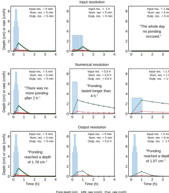
Second, the temporal resolution of the input data or put resolution is relevant for the modelled process. The in-put resolution of the forcing data can differ from the out-put resolution of the model, and this can impact the results of the model. An example is given in the upper panels of Fig. 2, showing an application of the Green–Ampt (Green and Ampt, 1911) infiltration model.
The numerical resolution (or the time step) of the model is the time interval over which the model calculates the states and the fluxes internally. A model can only deterministically resolve a process if the numerical resolution is higher than the characteristic timescale of the process. The panels in the
second row of Fig. 2 show how the numerical resolution im-pacts model output for the process of ponding, which leads to different conclusions about ponding, based on the model output.
The output resolution (often referred to as simply tempo-ral resolution) is the time interval at which the model output yields the states and fluxes. This time interval can be equal to the numerical resolution of the model, or aggregated from the numerical resolution. The modelled process can only be identified if the output time interval is shorter than the char-acteristic timescale of the process, which is shown in the lower panels of Fig. 2.
Input res. = 5 min Num. res. = 5 min Outp. res. = 5 min
Depth (cm) or rate (cm/h)
0 1 2 3 4
0 2 4 6
8 Input res. = 1 h Num. res. = 5 min Outp. res. = 5 min
Input resolution
0 1 2 3 4
0 2 4 6
8 Input res. = 1 dayNum. res. = 5 min Outp. res. = 5 min
"The whole day no ponding
occured."
0 1 2 3 4
0 2 4 6 8
Input res. = 5 min Num. res. = 5 min Outp. res. = 5 min
Depth (cm) or rate (cm/h)
"There was no more ponding after 2 h."
0 1 2 3 4
0 2 4 6
8 Input res. = 0.5 hNum. res. = 0.5 h Outp. res. = 0.5 h
Numerical resolution
"Ponding lasted longer than
4 h."
0 1 2 3 4
0 2 4 6
8 Input res. = 1 hNum. res. = 1 h Outp. res. = 1 h
0 1 2 3 4
0 2 4 6 8
Input res. = 5 min Num. res. = 5 min Outp. res. = 5 min
Depth (cm) or rate (cm/h)
Time (h) "Ponding reached a depth
of 1.78 cm."
0 1 2 3 4
0 2 4 6
8 Input res. = 5 minNum. res. = 5 min
Outp. res. = 0.5 h
Time (h) Output resolution
0 1 2 3 4
0 2 4 6
8 Input res. = 5 minNum. res. = 5 min
Outp. res. = 1 h
Time (h) "Ponding reached a depth
of 1.07 cm."
0 1 2 3 4
0 2 4 6 8
[image:4.612.127.468.68.459.2]Pond depth (cm) Infilt. rate (cm/h) Prec. rate (cm/h)
Figure 2. Application of the Green–Ampt infiltration scheme for different input resolutions (upper row), different numerical resolutions
(middle row), and different output resolutions (lower row). For each set-up, the model was fed with the same extreme precipitation event of 32 mm of rain in 30 min (4 mm in first 5 min, 5 mm in 5–10 min, 7 mm in 10–20 min, 5 mm in 20–25 min and 4 mm in 25–30 min). The
model parameters have been kept constant; saturated hydrologic conductivityKs=0.044 cm h−1, initial soil moistureθi=0.1, saturated
soil moistureθs=0.5, matric pressure at wetting front9=22.4 cm. Each of the three time concepts impacts the conclusions that are drawn
from the model results, which shows that calibration and validation at the appropriate time interval is essential to resolve the processes taking place.
Finally, the interpretation time interval is defined as the time interval at which the model output is eventually anal-ysed or interpreted. This can be equal to the calibration time interval, or the model output can be further aggregated re-sulting in a larger interpretation time interval (e.g. from daily to monthly). Since the model has not been validated or cali-brated on time intervals smaller than the calibration time in-terval, the credibility of the results will be unknown for time interval smaller than the calibration time interval.
It is critical to note that some of these time concepts are necessarily equal to or larger than related time concepts, sometimes for logical reasons (the output resolution can-not be higher than the numerical resolution) and sometimes
3 Example for VIC model studies
To illustrate the development of calibration/validation time interval and spatial resolution in large-domain hydrologi-cal modelling, we carried out a meta-analysis on the use of GHMs. The variable infiltration capacity (VIC) model (Liang et al., 1994) was chosen for this analysis because it is widely used and therefore enough studies were available for a meta-analysis. The VIC model is mentioned explicitly in Bierkens et al. (2014) as a type of model being run at the spatial hyper-resolution. Sub-grid variability is parameterized as a distri-bution of responses without explicit treatment of the pattern. We believe this model is representative of the much larger class of global hydrological models.
The VIC model was initially constructed to couple climate model output to hydrological processes: it is capable of solv-ing both the energy and the water balance. Lohmann et al. (1996) developed a horizontal routing model to couple the individual grid cells of the VIC model. This facilitated the distributed application of VIC for rainfall–runoff processes at large domains. No explicit definition of a spatial deriva-tive or scale appears in the equations of the VIC model, the spatial resolution of the model only appears in the routing scheme through the horizontal flow velocity (see Kampf and Burges (2007) for a description of space–time representation in other distributed hydrologic models).
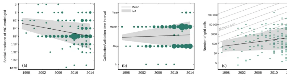
In our analysis we assembled 242 peer-reviewed stud-ies that used the VIC model. Of these, 192 studstud-ies used the model in a distributed way and performed a calibration or validation on the model output (see Table A1 in Ap-pendix A). Figure 3 presents a space–time perspective on the application of the VIC model during the past 2 decades. As expected, the spatial resolution at which the model is ap-plied has increased steadily over the years (Fig. 3a). While the model was initially constructed for spatial resolutions of the order of 0.5 to 2◦, it is now mostly applied at 1/8◦and smaller. The main driver for the increase in spatial resolution is the availability of high-resolution spatial data sets, such as that presented by Maurer et al. (2002). The increase in reso-lution, however, does not apply to the employed calibration and validation time interval. Figure 3b shows that the time interval at which the model has been calibrated and validated has remained steady over the years. Therefore, while the spa-tial resolution of the model has increased, the model output is still calibrated and validated at the original coarse time in-terval. Processes with a short timescale, which become more important when the spatial resolution increases, will likely be overlooked during the calibration and validation of the model if the time interval is too coarse. Several studies have already shown that calibration on a coarser time interval does not guarantee credible results for shorter time intervals (Melsen et al., 2015; Kavetski et al., 2011; Littlewood and Croke, 2013). There are, however, examples of studies where the in-terpretation time interval is smaller than the calibration time interval, e.g. Liu et al. (2013) and Costa-Cabral et al. (2013).
Figure 1 indicates the initial development scale of the VIC model (A), the scale where it is heading to right now (B), and the direction where it should go in order to resolve rele-vant hydrometeorological processes (C). Therefore, the VIC model with a high spatial resolution should be calibrated and/or validated at a time interval short enough to catch the processes relevant at those particular spatial scales.
Two causes for the discrepancy in the joint development of spatial resolutions and calibration time intervals come to mind: lack of computational power, or a lack of (using) ob-servations with a high temporal frequency. Figure 3c shows that the total number of grid cells that was used in the studies has on average increased over time. This is as ex-pected: computational power has increased significantly over the years. According to Moore’s law (Moore, 1965), com-putational power roughly doubles every 2 years. The grey lines in Fig. 3c indicate the corresponding slope in compu-tational power on a log–log scale. The largest numbers of grid cells per year likely indicate the limit of technical ca-pability. Overall, the trend in the studies, even in the higher quantiles, is much lower than the computational limit, sug-gesting that computational power is not a constraint for most studies. This implies that, presently, the main constraint for calibration and validation of distributed hydrological models at a certain time interval (Fig. 3b) is not the computational power, but the lack of (using) observations with a high tem-poral frequency. A possible explanation for this may be that many (global) studies rely on data from the Global Runoff Data Centre (GRDC), which are often available only at the monthly time interval. Also important is that for large basins, the typical application scale of VIC and other GHMs, flow is often regulated by dams for hydropower and flood control. Naturalized flows for these basins are often estimated at the monthly time interval. Our results reinforce the conclusion of Kirchner (2006) that field observations should account for the spatial and temporal heterogeneity of hydrometeorologi-cal processes, and the statement from Kavetski et al. (2011) that in most cases, temporal resolution is fixed by the data collection procedure.
4 Problem statement and outlook
The meta-anlysis on VIC studies showed that the spatial res-olution at which the model is applied has increased over the years, while the calibration time interval has remained steady (Fig. 3). The examples are shown for the VIC model only, but we have the impression that the obtained trends apply for all GHMs. There is a general tendency to move towards higher spatial resolution in large-domain hydrological mod-els (induced by e.g. Wood et al., 2011; Bierkens et al., 2014), whereas the available data for calibration and validation are model independent.
1998 2002 2006 2010 2014
1/128° 1/64° 1/32° 1/16° 1/8° 1/4° 1/2° 1° 2°
Year of publication
Spatial resolution of VIC model grid
(a)
1998 2002 2006 2010 2014 Year of publication
Calibration/validation time interval
h Day Month Year
(b) Mean SD
1998 2002 2006 2010 2014
Moore‘s Law
Year of publication
Number of grid cells
5 50 500 5000 50 000 500 000
[image:6.612.54.540.64.199.2](c)
Figure 3. The year of publication versus the highest spatial resolution of the VIC model that was used in the study (a), the smallest time
interval on which the calibration and/or validation of the VIC model was performed (b), and the total number of grid cells in the study (c) based on 192 peer-reviewed studies. The grey lines in (c) show the slope of computational power increase according to Moore’s law (Moore, 1965). The point size is proportional to the number of studies that were published in a certain year with a certain spatial or temporal resolution.
If the spatial resolution was given in kilometres, it was assumed that 1◦=100 km. For the total number of grid cells, catchment size was
divided by cell size, assuming that 1◦=100 km, unless the number of grid cells was explicitly given. Statistics (the mean and the standard
deviation) have been obtained per year on logarithmically transformed data. With linear regression a line was fitted through the mean and the standard deviation.
spatial hyper-resolution hydrological models with predictive capabilities should keep pace with the data that are required to run, calibrate, and validate the models. Increasing the spa-tial resolution of the model implies modelling different rele-vant hydrometeorological processes (there are some interest-ing developments concerninterest-ing parameter transferability over spatial resolutions; see e.g. Samaniego et al., 2010, Kumar et al., 2013, and Rakovec et al., 2015), which in turn requires calibration and validation to be performed on a smaller time interval. It requires a community effort to increase the avail-ability of high temporal resolution data for calibration and validation of large-domain hydrological models. Especially for large-domain studies, where data collection from all the separate basins at different institutes and countries is very time consuming (explaining the success of the GRDC), the data need to be gathered at and accessible from one point. It should also be recognized that discharge data only, especially at a monthly timescale, do not provide sufficient information for a process-based model evaluation at the spatial hyper-resolution scale. Possible paths forward are the use of tracer data to identify different flow paths (Tetzlaff et al., 2015), the use of multiple objectives (Gupta et al., 1998), and the use of satellite and remote sensing data (Pan et al., 2008), all at a representative spatial and temporal resolution.
We acknowledge that calibration and validation at the ap-propriate time interval is only one of the many challenges of spatial hyper-resolution hydrological modelling. Even with enough observations available for calibration and validation, disinformative data (Beven and Westerberg, 2011), correct subgrid parameterizations (Beven et al., 2015), and model structural uncertainty (Clark et al., 2015) remain outstand-ing challenges. However, we believe that all these challenges can only be tackled if the models are subject to critical and
process-based evaluation and validation (Gupta et al., 2008; Clark et al., 2011). In the end, the goal is to model hydrolog-ical processes in an appropriate way (Beven, 2006; McDon-nell et al., 2007).
Appendix A: Articles in the meta-analysis
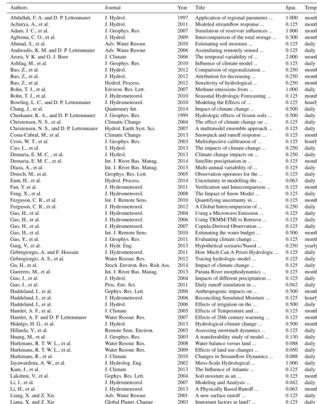
Table A1. All articles used to create Fig. 3, with their highest spatial resolution (Spat.; in degrees) and the time interval (Temp) used for
calibration and validation.
Authors Journal Year Title Spat. Temp.
Abdullah, F. A. and D. P. Lettenmaier J. Hydrol. 1997 Application of regional parameter ... 1.000 monthly
Acharya, A., et al. J. Hydrol. 2011 Modeled streamflow response ... 0.125 monthly
Adam, J. C., et al. J. Geophys. Res. 2007 Simulation of reservoir influences ... 1.000 monthly Agboma, C. O., et al. J. Hydrol. 2009 Intercomparison of the total storage ... 0.300 monthly
Ahmad, S., et al. Adv. Water Resour. 2010 Estimating soil moisture ... 0.125 daily
Andreadis, K. M. and D. P. Lettenmaier Adv. Water Resour. 2006 Assimilating remotely sensed ... 0.125 daily Arora, V. K. and G. J. Boer J. Climate 2006 The temporal variability of ... 2.000 monthly
Ashfaq, M., et al. J. Geophys. Res. 2010 Influence of climate model ... 0.125 daily
Bao, Z., et al. J. Hydrol. 2012 Comparison of regionalization ... 0.250 monthly
Bao, Z., et al. J. Hydrol. 2012 Attribution for decreasing ... 0.250 monthly
Bao, Z., et al. Hydrol. Process. 2012 Sensitivity of hydrological ... 0.250 monthly
Bohn, T. J., et al. Environ. Res. Lett. 2007 Methane emissions from ... 1.000 daily
Bohn, T. J., et al. J. Hydrometeorol. 2010 Seasonal Hydrologic Forecasting ... 0.125 monthly Bowling, L. C., and D. P. Lettenmaier J. Hydrometeorol. 2010 Modeling the Effects of ... 0.125 hourly
Chang, J., et al. Quaternary Int. 2014 Impact of climate change ... 0.500 daily
Cherkauer, K. A., and D. P. Lettenmaier J. Geophys. Res. 1999 Hydrologic effects of frozen soils ... 0.500 daily Christensen, N. S., et al. Climatic Change 2004 The effect of climate change on ... 0.125 daily Christensen, N. S., and D. P. Lettenmaier Hydrol. Earth Syst. Sci. 2007 A multimodel ensemble approach ... 0.125 daily Costa-Cabral, M., et al. Climatic Change 2013 Snowpack and runoff response ... 0.125 monthly Crow, W. T., et al. J. Geophys. Res. 2003 Multiobjective calibration of ... 0.125 hourly
Cuo, L., et al. J. Hydrol. 2013 The impacts of climate change ... 0.250 daily
Demaria, E. M. C. , et al. J. Hydrol. 2013 Climate change impacts on ... 0.250 daily
Demaria, E. M. C., et al. Int. J. River Bas. Manag. 2014 Satellite precipitation in ... 0.125 monthly Díaza, A., et al. Int. J. River Bas. Manag. 2013 Multi-annual variability of ... 0.125 daily Drusch, M., et al. Geophys. Res. Lett. 2005 Observation operators for the ... 0.125 daily
Eum, H., et al. Hydrol. Process. 2014 Uncertainty in modelling the ... 0.063 daily
Fan, Y. et al. J. Hydrometeorol. 2011 Verification and Intercomparison ... 0.125 monthly
Feng, X., et al. J. Hydrometeorol. 2008 The Impact of Snow Model ... 0.125 daily
Ferguson, C. R., et al. Int. J. Remote Sens. 2010 Quantifying uncertainty in ... 0.125 monthly Ferguson, C. R., et al. J. Hydrometeorol. 2012 A Global Intercomparison of ... 0.250 daily
Gao, H., et al. J. Hydrometeorol. 2004 Using a Microwave Emission ... 0.125 daily
Gao, H., et al. J. Hydrometeorol. 2006 Using TRMM/TMI to Retrieve ... 0.125 daily
Gao, H., et al. J. Hydrometeorol. 2007 Copula-Derived Observation ... 0.125 daily
Gao, H., et al. Int. J. Remote Sens. 2010 Estimating the water budget ... 0.500 monthly
Gao, Y., et al. J. Geophys. Res. 2011 Evaluating climate change ... 0.125 monthly
Garg, V., et al. J. Hydr. Eng. 2013 Hypothetical scenario?based ... 0.250 yearly
Gebregiorgis, A. and F. Hossain J. Hydrometeorol. 2011 How Much Can A Priori Hydrologic ... 0.125 daily Gebregiorgis, A. S., et al. Water Resour. Res. 2012 Tracing hydrologic model ... 0.125 daily Gu, H., et al. Stoch. Environ. Res. Risk Ass. 2014 Impact of climate change ... 0.125 daily Guerrero, M., et al. Int. J. River Bas. Manag. 2013 Parana River morphodynamics ... 0.125 monthly
Guo, J., et al. J. Hydrol. 2004 Impacts of different precipitation ... 0.125 daily
Guo, J., et al. Proc. Env. Sci. 2011 Daily runoff simulation in ... 0.042 daily
Haddeland, I., et al. Gephys. Res. Lett. 2006 Anthropogenic impacts on ... 0.500 monthly Haddeland, I., et al. J. Hydrometeorol. 2006 Reconciling Simulated Moisture ... 0.125 hourly
Haddeland, I., et al. J. Hydrol. 2006 Effects of irrigation on the ... 0.500 daily
Hamlet, A. F., et al. J. Climate 2005 Effects of Temperature and ... 0.125 monthly
Hamlet, A. F. and D. P. Lettenmaier Water Resour. Res. 2007 Effects of 20th century warming ... 0.125 monthly
Hidalgo, H. G., et al. J. Hydrol. 2013 Hydrological climate change ... 0.500 monthly
Hillarda, Y., et al. Remote Sens. Environ. 2003 Assessing snowmelt dynamics ... 0.125 daily Huang, M., et al. J. Geophys. Res. 2003 A transferability study of model ... 0.130 daily Hurkmans, R. T. W. L., et al. Water Resour. Res. 2008 Water balance versus land ... 0.088 daily Hurkmans, R. T. W. L., et al. Water Resour. Res. 2009 Effects of land use changes ... 0.050 daily
Hurkmans, R., et al. J. Climate 2010 Changes in Streamflow Dynamics ... 0.088 daily
Jayawardena, A. W., et al. J. Hydrolog. Eng. 2002 Meso-Scale Hydrological ... 1.000 daily
Kam, J., et al. J. Climate 2013 The Influence of Atlantic ... 0.125 daily
Lakshmi, V., et al. Gephys. Res. Lett. 2004 Soil moisture as an ... 0.125 monthly
Li, J., et al. J. Hydrometeorol. 2007 Modeling and Analysis ... 0.042 daily
Li, H., et al. J. Hydrometeorol. 2013 A Physically Based Runoff ... 0.063 monthly
Liang, X. and Z. Xie Adv. Water Resour. 2001 A new surface runoff ... 0.125 daily
Liang, X. and Z. Xie Global Planet. Change 2003 Important factors in land? ... 0.125 daily
Authors Journal Year Title Spat. Temp.
Authors Journal Year Title Spat. Temp. Shrestha, R. R., et al. Hydrol. Process. 2012 Modelling spatial and ... 0.063 monthly Shrestha, K. Y., et al. J. Hydrometeorol. 2014 An Atmospheric-Hydrologic ... 0.250 daily Shrestha, R. R., et al. J. Hydrometeorol. 2014 Evaluating Hydroclimatic ... 0.063 daily Shrestha, R. R., et al. Hydrol. Process. 2014 Evaluating the ability of a ... 0.063 monthly Shukla, S., et al. Hydrol. Earth Syst. Sci. 2012 Value of medium range ... 0.500 2-weeks Shukla, S., et al. Hydrol. Earth Syst. Sci. 2012 On the sources of global land ... 0.500 monthly Sinha, T., et al. J. Hydrometeorol. 2010 Impacts of Historic Climate ... 0.125 weekly Sinha, T. and K. A. Cherkauer J. Geophys. Res. 2010 Impacts of future climate ... 0.125 weekly Sinha, T. and A. Sankarasubramanian Hydrol. Earth Syst. Sci. 2013 Role of climate forecasts and ... 0.125 monthly Slater, A. G., et al. J. Geophys. Res. 2007 A multimodel simulation of ... 1.000 monthly Sridhar, V., et al. Climate Dynamics 2013 Explaining the hydroclimatic ... 0.125 monthly Stephen, H., et al. Hydrol. Earth Syst. Sci. 2010 Relating surface backscatter ... 0.125 daily
Su, F., et al. J. Geophys. Res. 2005 Streamflow simulations of ... 1.000 monthly
Su, F., et al. J. Geophys. Res. 2006 Evaluation of surface water ... 1.000 monthly
Su, F., et al. J. Hydrometeorol. 2008 Evaluation of TRMM Multisatellite ... 0.125 daily Su, F. and D. P. Lettenmaier J. Hydrometeorol. 2009 Estimation of the Surface ... 0.125 monthly Tang, C. and T. C. Piechota J. Hydrol. 2009 Spatial and temporal soil ... 0.125 monthly Tang, Q. and D. P. Lettenmaier Int. J. Remote Sens. 2010 Use of satellite snow-cover ... 0.063 monthly
Tang, C., et al. J. Hydrol. 2011 Relationships between ... 0.125 monthly
Tang, Q., et al. J. Hydrometeorol. 2012 Predictability of Evapotranspiration ... 0.063 daily Tang, C., et al. Global Planet. Change 2012 Assessing streamflow sensitivity ... 0.063 monthly Tang, C. and R. L. Dennis Global Planet. Change 2014 How reliable is the offline ... 0.125 monthly Vano, J. A. et al. J. Hydrometeorol. 2012 Hydrologic Sensitivities of ... 0.125 monthly VanShaar, J. R. et al. Hydrol. Process. 2012 Effects of land-cover changes ... 0.125 monthly Vicuna, S. et al. J. Am. Water Resour. As. 2007 The sensitivity of California ... 0.125 monthly Voisin, N., et al. J. Hydrometeorol. 2008 Evaluation of Precipitation ... 0.500 monthly Voisin, N.,et al. Weather Forecast. 2011 Application of a Medium-Range ... 0.250 daily Wang, A., et al. J. Geophys. Res. 2008 Integration of the variable ... 0.125 monthly Wang, J., et al. Int. J. Clim. 2010 Quantitative assessment of climate ... 0.125 monthly Wang, G .Q, et al. Hydrol. Earth Syst. Sc. 2012 Assessing water resources in ... 0.500 daily Werner, A. T., et al. Atmosphere-Ocean 2013 Spatial and Temporal Change ... 0.063 daily
Wen, Z., et al. Water Resour. Res. 2012 A new multiscale routing ... 0.031 daily
Wenger, S. J., et al. Water Resour. Res. 2010 Macroscale hydrologic ... 0.063 daily Wojcik, R., et al. J. Hydrometeorol. 2008 Multimodel Estimation of ... 0.125 hourly
Wood, A. W., et al. J. Geophys. Res. 2002 Long-range experimental ... 0.125 monthly
Wood, A. W., et al. J. Geophys. Res. 2005 A retrospective assessment ... 0.125 monthly
Wu, Z., et al. Atmosphere-Ocean 2007 Thirty-Five Year (1971–2005) ... 0.300 daily
Wu, Z. Y., et al. Hydrol. Earth Syst. Sci. 2011 Reconstructing and analyzing ... 0.300 daily
Wu, H., et al. Water Resour. Res. 2014 Real-time global flood ... 0.125 daily
Xia, Y., et al. J. Geophys. Res. 2012 Continental-scale water ... 0.125 daily
Xia, Y., et al. Hydrol. Process. 2012 Comparative analysis of ... 0.125 monthly
Xia, Y., et al. Hydrol. Process. 2014 Evaluation of NLDAS-2 ... 0.125 daily
Xie, Z., et al. J. Hydrometeorol. 2007 Regional Parameter Estimation ... 0.500 monthly
Yang, G., et al. J. Hydrometeorol. 2010 Hydroclimatic Response of ... 0.125 daily
Yang, G., et al. Landscape Urban Plan. 2011 The impact of urban development ... 0.125 daily Yang, G. and L. C. Bowling Water Resour. Res. 2014 Detection of changes in ... 0.125 daily
Yearsley, J. Water Resour. Res. 2012 A grid-based approach for ... 0.063 daily
Yong, B., et al. Water Resour. Res. 2010 Hydrologic evaluation of ... 0.063 daily
Yong, B., e al. J. Hydrometeorol. 2013 Spatial-Temporal Changes of ... 0.063 daily Yuan, F., et al. Can. J. Remote Sens. 2004 An application of the VIC-3L ... 0.250 daily
Yuan, X., et al. Hydr. Sci. J. 2009 Sensitivity of regionalized ... 0.500 monthly
Yuan, X., et al. J. Hydrometeorol. 2013 Probabilistic Seasonal ... 0.250 monthly
Zeng, X., et al. J. Hydrometeorol. 2010 Comparison of Land?Precipitation ... 0.125 monthly
Zhang, X., et al. Phys. Chem. Earth 2012 Modeling and assessing ... 0.031 monthly
Zhang, B., et al. Agr. Water Manage. 2012 Drought variation trends in ... 0.500 yearly Zhang, B., et al. Theor. Appl. Climatol. 2013 A drought hazard assessment ... 0.500 yearly Zhang, B., et al. Hydrol. Process. 2014 Assessing the spatial and ... 0.500 yearly
Zhang, X., et al. J. Hydrometeorol. 2014 A Long-Term Land Surface ... 0.250 monthly
Zhang, B., et al. Hydrol. Process. 2014 Spatiotemporal analysis of climate ... 0.500 yearly Zhao, F., et al. J. Hydrometeorol. 2012 Application of a Macroscale ... 0.050 daily Zhao, X. and P. Wu Natural Hazards 2013 Meteorological drought over ... 0.500 yearly Zhao, Q., et al. Env. Earth Sci. 2013 Coupling a glacier melt model ... 0.083 daily
Zhao, F., et al. J. Hydrol. 2013 The effect of spatial rainfall ... 0.050 daily
Acknowledgements. The authors would like to thank Claudia Brauer and Massimiliano Zappa for their useful suggestions concerning a draft version of this paper.
Edited by: E. Zehe
References
Anderson, M. and Burt, T.: Process Studies in Hillslope Hydrology, chap. Subsurface runoff, 365–400, Wiley, 1990.
Arora, V., Chiew, F., and Grayson, R.: Effect of sub-grid-scale variability of soil moisture and precipitation intensity on sur-face runoff and streamflow, J. Geophys. Res., 106, 17073–17091, doi:10.1029/2001JD900037, 2001.
Bastiaanssen, W., Allen, R., Droogers, P., D’Urso, G., and Ste-duto, P.: Twenty-five years modeling irrigated and drained soils: State of the art, Agr. Water Manage., 92, 111–125, doi:10.1016/j.agwat.2007.05.013, 2007.
Beven, K.: Linking parameters across scales: subgrid parameteriza-tions and scale dependent hydrological models, Hydrol. Process., 9, 507–525, doi:10.1002/hyp.3360090504, 1995.
Beven, K.: Searching for the Holy Grail of scientific hydrology:
Qt=(S, R, 1t )Aas closure, Hydrol. Earth Syst. Sci., 10, 609–
618, doi:10.5194/hess-10-609-2006, 2006.
Beven, K. and Cloke, H.: Comment on “Hyperresolution global land surface modeling: Meeting a grand challenge for monitoring Earth’s terrestrial water” by Eric F. Wood et al., Water Resour. Res., 48, W01801, doi:10.1029/2011WR010982, 2012. Beven, K. and Westerberg, I.: On red herrings and real herrings:
dis-information and dis-information in hydrological inference, Hydrol. Process., 25, 1676–1680, doi:10.1002/hyp.7963, 2011.
Beven, K., Cloke, H., Pappenberger, F., Lamb, R., and Hunter, N.: Hyperresolution information and hyperresolution ignorance in modelling the hydrology of the land surface, Sc. China: Earth Sc., 58, 25–35, doi:10.1007/s11430-014-5003-4, 2015. Beven, K. J.: Rainfall-Runoff modelling, The Primer – 2nd Edition,
vol. Ch.1. Down to Basics: Runoff Processes and the Modelling Process, John Wiley & Sons, 2012.
Bierkens, M., Finke, P., and De Willigen, P.: Upscaling and Down-scaling Methods for Environmental Research, Springer, London, UK, 2000.
Bierkens, M., Bell, V., Burek, P., Chaney, N., Condon, L., David, C., De Roo, A., Döll, P., Drost, N., Famiglietti, J., Flörke, M., Gochis, D., Houser, P., Hut, R., Keune, J., Kollet, S., Maxwell, R., Reager, J., Samaniego, L., Sudicky, E., Sutanudjaja, E., Van de Giesen, N., Winsemius, H., and Wood, E.: Hyper-resolution global hydrological modelling: What’s next?, Hydrol. Process., 29, 310–320, doi:10.1002/hyp.10391, 2014.
Bierkens, M. F. P.: Global hydrology 2015: State, trends,
and directions, Water Resour. Res., 51, 4923–4947,
doi:10.1002/2015WR017173, 2015.
Blöschl, G. and Sivapalan, M.: Scale issues in hydrolog-ical modelling: a review, Hydrol. Process., 9, 251–290, doi:10.1002/hyp.3360090305, 1995.
Boyle, D., Gupta, H., Sorooshian, S., Koren, V., Zhang, Z., and Smith, M.: Towards improved streamflow forecasts: Value of semidistributed modeling, Water Resour. Res., 37, 2749–2759, doi:10.1029/2000WR000207, 2001.
Brutsaert, W.: Hydrology: An Introduction, Cambridge University Press, 2005.
Clark, M., McMillan, H., Collins, D., Kavetski, D., and Woods, R.: Hydrological field data from a modeller’s perspective: Part 2: process-based evaluation of model hypotheses, Hydrol. Process., 25, 523–543, doi:10.1002/hyp.7902, 2011.
Clark, M., Nijssen, B., Lundquist, J., Kavetski, D., Rupp, D., Woods, R., Freer, J., Gutmann, E., Wood, A., Brekke, L. D., Arnold, J., Gochis, D., and Rasmussen, R.: A unified approach for process-based hydrologic modeling: 1. Modeling concept, Water Res. Res., 51, 2498–2514, doi:10.1002/2015WR017198, 2015.
Costa-Cabral, M., Roy, S., Maurer, E., Mills, W., and Chen, L.: Snowpack and runoff response to climate change in Owens Val-ley and Mono Lake watersheds, Clim. Change, 116, 97–109, doi:10.1007/s10584-012-0529-y, 2013.
Dooge, J.: Reflections in Hydrology: Science and Practice, chap. Scale problems in hydrology, Kiesel Memorial Lecture, 85–145, American Geophysical Union, Washington D.C., 1986. Dooge, J.: Hydrology in Perspective, Hydr. Sci. J., 33, 61–85, 1988. Dunne, T.: Hillslope Hydrology, chap. Field studies of hillslope
flow processes, 227–293, Wiley, 1978.
Fearn, N.: Zeno and the Tortoise: How to think like a philosopher, Atlantic Books, London, Great Brittain, 2001.
Feddes, R. (Ed.): Space and Time scale variability and interdepen-dencies in hydrological processes, Cambridge University Press, 1995.
Fortak, H. (Ed.): Meteorologie, Dietrich Reimer, Berlin, 1982. Gentine, P., Troy, T., Lintner, B., and Findell, K.: Scaling in Surface
Hydrology: Progress and Challenges, Journal of Contemporary Water Research & Education, 147, 28–40, 2012.
Gray, W., Leijnse, A., Kolar, R., and Blain, C.: Mathematical Tools for Changing Scale in the Analysis of Physical Systems, CRC Press, 1993.
Green, W. and Ampt, G.: Studies of soil physics, part I – the flow of water and air through soils, J. Agr. Sci., 4, 1–24, doi:10.1017/S0021859600001441, 1911.
Gupta, H., Sorooshian, S., and Yapo, P.: Toward improved cal-ibration of hydrologic models: Multiple and noncommensu-rable measures of information, Water Resour. Res., 34, 751–763, doi:10.1029/97WR03495, 1998.
Gupta, H., Wagener, T., and Liu, Y.: Reconciling theory with obser-vations: elements of a diagnostic approach to model evaluation, Hydrol. Process., 22, 3802–3813, doi:10.1002/hyp.6989, 2008. Gupta, V., Rodríguez-Iturber, I., and Wood, E. (Eds.): Scale
prob-lems in hydrology, D. Reidel Publishing Company, 1986. Kalma, J. and Sivapalan, M. (Eds.): Advances in Hydrological
Pro-cesses – Scale issues in Hydrological modelling, John Wiley & Sons, 1995.
Kampf, S. and Burges, S.: A framework for classifying and compar-ing distributed hillslope and catchment hydrologic models, Water Resour. Res., 43, W05423, doi:10.1029/2006WR005370, 2007. Kavetski, D., Fenicia, F., and Clark, M. P.: Impact of
tempo-ral data resolution on parameter inference and model iden-tification in conceptual hydrological modeling: Insights from an experimental catchment, Water Resour. Res., 47, W05501, doi:10.1029/2010WR009525, 2011.
Water Resour. Res., 32, 1699–1712, doi:10.1029/96WR00603, 1996.
Kirchner, J.: Getting the right answers for the right reasons: Linking measurements, analyses, and models to advance the science of hydrology, Water Resour. Res., 42, W03S04, doi:10.1029/2005WR004362, 2006.
Klemeš, V.: Conceptualization and scale in hydrology, J. Hydrol., 65, 1–23, 1983.
Kumar, R., Samaniego, L., and Attinger, S.: Implications of dis-tributed hydrologic model parameterization on water fluxes at multiple scales and locations, Water Resour. Res., 49, 360–379, doi:10.1029/2012WR012195, 2013.
Liang, X., Lettenmaier, D. P., Wood, E. F., and Burges, S. J.: A simple hydrologically based model of land surface water and en-ergy fluxes for general circulation models, J. Geophys. Res., 99, 14415–14458, 1994.
Littlewood, I. and Croke, B.: Effects of data time-step on the accu-racy of calibrated rainfall-streamflow model parameters: practi-cal aspects of uncertainty reduction, Hydrol. Res., 44, 430–440, doi:10.2166/nh.2012.099, 2013.
Liu, H., Tian, F., Hu, H. C., Hu, H. P., and Sivapalan, M.: Soil mois-ture controls on patterns of grass green-up in Inner Mongolia: an index based approach, Hydrol. Earth Syst. Sci., 17, 805–815, doi:10.5194/hess-17-805-2013, 2013.
Liu, Y. and Gupta, H. V.: Uncertainty in hydrologic modeling: To-wards an integrated data assimilation framework, Water Resour. Res., 43, W07401, doi:10.1029/2006WR005756, 2007. Lohmann, D., Nolte-Holube, R., and Raschke, E.: A large-scale
hor-izontal routing model to be coupled to land surface parameteri-zation schemes, Tellus, 48A, 708–721, 1996.
Maurer, E., Wood, A., Adam, J., Lettenmaier, D., and Nijssen, B.: A Long-Term Hydrologically Based Dataset of Land Surface Fluxes and States for the Conterminous United States, J. Climate, 15, 3237–3251, doi:10.1175/JCLI-D-12-00508.1, 2002. McDonnell, J. and Beven, K.: Debates – The future of
hydrologi-cal sciences: A (common) path forward? A hydrologi-call to action aimed at understanding velocities, celerities and residence time distri-butions of the headwater hydrograph, Water Resour. Res., 50, 5342–5350, doi:10.1002/2013WR015141, 2014.
McDonnell, J., Sivapalan, M., Vaché, K., Dunn, S., Grant, G., Hag-gerty, R., Hinz, C., Hooper, R., Kirchner, J., Roderick, M. L., Selker, J., and Weiler, M.: Moving beyond heterogeneity and pro-cess complexity: A new vision for watershed hydrology, Water Resour. Res., 43, W07301, doi:10.1029/2006WR005467, 2007. Melsen, L., Teuling, A., Torfs, P., Zappa, M., Mizukami, N., Clark,
M., and Uijlenhoet, R.: Representation of spatial and temporal variability in large-domain hydrological models: Case study for a mesoscale prealpine basin, Hydrol. Earth Syst. Sci. Discuss., doi:10.5194/hess-2015-532, in review, 2016.
Montaldo, N. and Albertson, J.: Temporal dynamics of soil mois-ture variability: 2. Implications for land surface models, Water Resour. Res., 39, 1275, doi:10.1029/2002WR001618, 2003. Moore, G. E.: Cramming More Components onto Integrated
Cir-cuits, Electronics, April, 114–117, 1965.
Orlanski, I.: A rational subdivision of scales for atmospheric pro-cesses, B. Am. Meteorol. Soc., 56, 527–530, 1975.
Pan, M., Wood, E., Wójcik, R., and McCabe, M.: Estimation of regional terrestrial water cycle using multi-sensor remote sensing observations and data assimilation, Remote Sens. Environ., 112, 1282–1294, doi:10.1016/j.rse.2007.02.039, 2008.
Rakovec, O., Kumar, R., Mai, J., Cuntz, M., Thober, S., Zink, M., Attinger, S., Schäfer, D., Schrön, M., and Samaniego, L.: Mul-tiscale and multivariate evaluation of water fluxes and states over European river basins, J. Hydrometeorol. 17, 287–307, doi:10.1175/JHM-D-15-0054.1, 2015.
Reggiani, P., Sivapalan, M., and Hassanizadeh, S.: A unifying framework for watershed thermodynamics: balance equations for mass, momentum, energy and entropy, and the second law of thermodynamics, Adv. Water. Resour., 22, 367–398, doi:10.1016/S0309-1708(98)00012-8, 1998.
Samaniego, L., Kumar, R., and Attinger, S.: Multiscale pa-rameter regionalization of a grid-based hydrologic model
at the mesoscale, Water Resour. Res., 46, W05523,
doi:10.1029/2008WR007327, 2010.
Sposito, G. (Ed.): Scale dependence and scale invariance in hydrol-ogy, Cambridge University Press, 1998.
Stillwell, J.: Mathematics and its History, Springer, 1989.
Stommel, H.: Varieties of Oceanographic Experience, Science, 139, 572–576, 1963.
Tetzlaff, D., Buttle, J., Carey, S. K., McGuire, K., Laudon, H., and Soulsby, C.: Tracer-based assessment of flow paths, storage and runoff generation in northern catchments: a review, Hydrol. Pro-cess., 29, 3475–3490, doi:10.1002/hyp.10412, 2015.
Todini, E.: Rainfall-runoff modeling – past, present and future, J. Hydrol., 100, 341–352, doi:10.1016/0022-1694(88)90191-6, 1988.
Wagener, T. and Gupta, H.: Model identification for hydrological forecasting under uncertainty, Stoch. Env. Res. Risk A., 19, 378– 387, doi:10.1007/s00477-005-0006-5, 2005.
Whitaker, S.: Theory and Applications of Transport in Porous Me-dia: The Method of Volume Averaging, Springer, 1999. Wood, E., Sivapalan, M., Beven, K., and Band, L.: Effects of spatial
variability and scale with implications to hydrologic modeling, J. Hydrol., 102, 29–47, 1988.
Wood, E., Lettenmainer, D., and Zartarian, V.: A Land-Surface Hydrology Parameterization With Subgrid Variability for Gen-eral Circulation Models, J. Geophys. Res., 97, 2717–2728, doi:10.1029/91JD01786, 1992.