Study of Nonlinear Evolution Equations to Construct Traveling Wave Solutions via the New Approach of the Generalized (G'/G) Expansion Method

Study of Nonlinear Evolution Equations to Construct

Traveling Wave Solutions via the New Approach of the

Generalized

(

G

′

/

G

)

-Expansion Method

Md. Nur Alam

1,*

_{, M. Ali Akbar}

2

_{, Harun-Or-Roshid}

1

1_{Department of Mathematics, Pabna University of Science and Technology, Bangladesh} 2_{Department of Applied Mathematics, University of Rajshahi, Bangladesh}

*Corresponding Author: [email protected]

Copyright © 2013 Horizon Research Publishing All rights reserved.

Abstract

Exact solutions of nonlinear evolution equations (NLEEs) play very important role to make known the inner mechanism of compound physical phenomena. In this paper, the new generalized (G′/G)-expansion method is used for constructing the new exact traveling wave solutions for some nonlinear evolution equations arising in mathematical physics namely, the (3+1)-dimensional Zakharov-Kuznetsov equation and the Burgers equation. As a result, the traveling wave solutions are expressed in terms of hyperbolic, trigonometric and rational functions. This method is very easy, direct, concise and simple to implement as compared with other existing methods. This method presents a wider applicability for handling nonlinear wave equations. Moreover, this procedure reduces the large volume of calculations.

Keywords

The New Generalized (G′/G)-Expansion Method; The (3+1)-Dimensional Zakharov-Kuznetsov Equation And The Burgers Equation; Traveling Wave Solutions; Solitary Wave Solutions

1. Introduction

The investigation of the travelling wave solutions for nonlinear partial differential equations plays an important role in the study of nonlinear physical phenomena. Nonlinear wave phenomena appears in various scientific and engineering fields, such as fluid mechanics, plasma physics, optical fibers, biology, solid state physics, chemical kinematics, chemical physics and geochemistry. Nonlinear wave phenomena of dispersion, dissipation, diffusion, reaction and convection are very important in nonlinear wave equations. In the past several decades, new exact solutions may help to find new phenomena. A variety of powerfull methods, such as the ansatz method [1, 2], the Adomian decomposition method [3], the Darboux transformation method [4], the Backlund transformation method [5], the inverse scattering transform [6], the wave of

translation method [7], the Jacobi elliptic function method [8-11], the Exp-function method [12-17], the extended tanh method [18, 19], the sine-cosine method [20], the Cole-Hopf transformation [21], the (G′/G)-expansion method [22-30], the modified simple equation method [31, 32], the novel

) /

(G′ G _{-expansion method [33] and so on.}

Recently, Naher and Abdullah [34] established a highly effective extension of the

(

G

′

/

G

)

- expansion method, called the new generalized

(

G

′

/

G

)

-expansion method to obtain exact traveling wave solutions of NLEEs. The objective of this article is to look for new study relating to the new generalized

(

G

′

/

G

)

-expansion method to examine exact solutions to the celebrated Burgers equation and the (3+1)- dimensional ZK equations to establish the advantages and effectiveness of the method. The Burgers equation is used to capture some of the features of turbulent fluid in a channel caused by the interaction of the opposite effects of convection and diffusion. The (3+1)-dimensional Zakharov–Kuznetsov equation describes weakly nonlinear wave process in dispersive and isotropic media e.g., waves in magnetized plasma or water waves in shear flows.

The rest of the article is organized as follows: In Section 2, the description of the new generalized

(

G

′

/

G

)

expansion method is given. In Section 3, we apply the method to obtain the traveling wave solution of the (3+1)-dimensional Zakharov-Kuznetsov equation and the Burgers equation and also give some discussion, Graphical representation and Table. In Sections 4, we give some conclusions.

2. Materials and Methods

Let us consider a general nonlinear PDE in the form

0

)

,

,

,

,

,

,

(

u

u

t

u

x

u

tt

u

tx

u

xx



=

P

(1)

where u=u(x,t) is an unknown function, P is a polynomial in u(x,t)and its derivatives in which highest order derivatives and nonlinear terms are involved and the subscripts stand for the partial derivatives.

complex variable

η

,

) ( ) ,

(x t u

η

u = ,

η

=x±Vt (2) where V is the speed of the traveling wave. The traveling wave transformation (2) converts Eq. (1) into an ordinary differential equation (ODE) for u=u(

η

):

0 ) , , , ,

(_{u u}′_u′′_u′′′_ =

Q (3)

where Q is a polynomial of

u

and it derivatives and the superscripts indicate the ordinary derivatives with respect to

η

.

Step 2: According to possibility, Eq. (3) can be integrated term by term one or more times, yields constant(s) of integration. The integral constant may be zero for simplicity.

Step 3: Suppose the traveling wave solution of Eq. (3) can be expressed as follows:

i N

i i i

N

i

i

d

H

d

H

u

−

= =

+

+

+

=

∑

(

)

∑

(

)

)

(

1 0

β

α

η

(4)

where either

α

_N or

β

_N may be zero, but both

α

_N or

N

β

could be zero at a time,

α

_i (i=0,1,2,,N) and

β

_i

) , , 2 , 1

(i=  N and d are arbitrary constants to be determined later and H(

η

) is given by

)

/

(

)

(

G

G

H

η

=

′

₍₅₎ where G=G(

η

) satisfies the following auxiliary nonlinear ordinary differential equation:

0 ) ( 2

2_{− ′ =}

− ′ −

′′ _{BGG EG C G}

G

AG (6)

where the prime stands for derivative with respect to

η

; A, B,C and E are real parameters.

Step 4: To determine the positive integer N, taking the homogeneous balance between the highest order nonlinear terms and the derivatives of the highest order appearing in Eq. (3).

Step 5: Substitute Eq. (4) and Eq. (6) including Eq. (5) into Eq. (3) with the value of

N

obtained in Step 4, we obtain polynomials in _(d+H)N _{(N=0,1,2,) and}

N

H d_{+ )}−

( (N =0,1,2,) . Then, we collect each coefficient of the resulted polynomials to zero yields a set of algebraic equations for

α

_i (i=0,1,2,,N) and

β

i

) , , 2 , 1

(i=  N , d and V.

Step 6: Suppose that the value of the constants

α

_i

) , , 2 , 1 , 0

(i=  N ,

β

i (i=1,2,,N),

d

and

V

can be

found by solving the algebraic equations obtained in Step 5. Since the general solution of Eq. (6) is well known to us, inserting the values of

α

i (i=0,1,2,,N) ,

β

i

) , , 2 , 1

(i=  N ,d and V into Eq. (4), we obtain more general type and new exact traveling wave solutions of the nonlinear partial differential equation (1).

Using the general solution of Eq. (6), we have the following solutions of Eq. (5):

Family 1: When

B

≠

0

,

ψ

= A−C and

, 0 ) ( 4

2_{+ − >}

=

Ω B E A C















 Ω

+















 Ω















 Ω

+















 Ω

×

Ω

+

=











 ′

=

η

η

η

η

ψ

ψ

η

A

C

A

C

A

C

A

C

B

G

G

H

2

sinh

2

cosh

2

cosh

2

sinh

2

2

)

(

2 1

2

1 (7)

Family 2: When

B

≠

0

,

ψ

=A−C and

, 0 ) ( 4

2 _{+ − <}

=

Ω B E A C

    

 

 _−Ω

+     

 

 _−Ω

    

 

 −Ω

+     

 

 −Ω

− ×

Ω − + =       ′ =

η

η

η

η

ψ

ψ

η

A C

A C

A C

A C

B G G H

2 sin 2

cos

2 cos 2

sin

2 2 )

(

2 1

2

1 (8)

Family 3: When

B

≠

0

,

ψ

=A−C and

, 0 ) ( 4

2 _{+ − =}

=

Ω B E A C

η

ψ

η

2 1

2

2 )

(

C C

C B

G G H

+ + =       ′

= ₍₉₎

Family 4: When

B

=

0

,

ψ

=A−C and ∆=

ψ

E>0,

)

sinh(

)

cosh(

)

cosh(

)

sinh(

)

(

2 1

2 1

η

η

η

η

ψ

η

A

C

A

C

A

C

A

C

G

G

H

∆

+

∆

∆

+

∆

×

∆

=











 ′

=

(10)

Family 5: When

B

=

0

,

ψ

= A−C and ∆=

ψ

E<0,

)

sin(

)

cos(

)

cos(

)

sin(

)

(

2 1

2 1

η

η

η

η

ψ

η

A

C

A

C

A

C

A

C

G

G

H

∆

−

+

∆

−

∆

−

+

∆

−

−

×

∆

−

=











 ′

=

(11)

3. Applications of the Method

Zakharov-Kuznetsov equation and the Burgers equation which are very important nonlinear evolution equations in applied sciences. The obtained solutions and the solutions obtained in previous literature have been compared and discussed in this section. Furthermore, the obtained solutions are demonstrated in graphs by using the symbolic computation software.

3.1. Application of the Method

Now we will study the new generalized (G′/G)

expansion method to find exact solutions and then the solitary wave solutions to the (3+1)-dimensional ZK equation. Let us consider the (3+1)-dimensional ZK equation,

0

=

+

+

+

+

_{x xx yy zz}

t

auu

u

u

u

u

(12)

We utilize the traveling wave variable S(

η

)=u(x,y,z,t), Vt

z y x+ + − =

η

, Eq. (12) is carried to an ODE

0

3

′′

=

+

′

+

′

−

V

S

aS

S

S

(13) Eq. (13) is integrable, therefore, integrating with respect to

η

once yields:

, 0 3 2

1 2 _{+ ′=} +

−VS aS S

P (14)

where P is an integration constant which is to be determined.

Taking the homogeneous balance between highest order nonlinear term _S2 _{and linear term of the highest order S′}

in Eq. (14), we obtain N=1. Therefore, the solution of Eq. (14) is of the form:

, ) ( ) ( )

( 1

1 1

0 + + + + −

= d M d M

v

η

α

α

β

(15)

where

α

₀,

α

₁,

β

₁ and d are constants to be determined. Substituting Eq. (15) together with Eqs. (5) and (6) into Eq.(14), the left-hand side is converted into polynomials in

(

_d+M

)

N _{(N =01,,2,...)}

and

(

_d+M

)

−N _{(N=1, 2,)}

.

We collect each coefficient of these resulted polynomials to zero yields a set of simultaneous algebraic equations (for simplicity, the equations are not presented) for

α

₀,

α

₁,

β

₁,

d, P and V . Solving these algebraic equations with the help of computer algebra, we obtain following:

Set 1:

)

12

6

12

36

36

36

(

2

1

0 0

2 0

2 2 0 2 2

2 2

ACd

a

AB

a

d

A

a

A

a

Bd

d

E

aA

P

α

α

α

α

ψ

ψ

ψ

+

−

−

+

+

+

−

=

0

0

α

α

= , 1( 6d a ₀A 3B),

A

V = −

ψ

+

α

−

d

=

d

,

α

₁=0,

), (

6 2

1 =−_aA −E+d

ψ

+Bd

β

(16)

where

ψ

=

A

−

C

,

α

₀

,

d

,

A

,

B

,

C E

,

are free parameters.

Set 2:

) 6

12 12

36 36

36 ( 2

1

0 2

0 0

2 2 0 2 2 2 2

AB a d A a ACd a

E A

a d

Bd aA

P

α

α

α

ψ

α

ψ

ψ

+ +

−

− +

+ =

0

0

α

α

= , 1(a ₀A 6d 3B),

A

V =

α

+

ψ

+

d

=

d

,

, 0

1 =

β

aA

ψ

α

₁=6 (17)

where

ψ

=

A

−

C

,

α

₀

,

d

,

A

,

B

,

C E

,

are free parameters.

Set 3:

) 36 144

( 2

1 2 2 2

0 2

2 a A E B

aA

P=

α

−

ψ

− ,V =a

α

₀,

ψ

2

B

d =− ,

α

₀ =

α

₀, ₁ 6 ,

aA

ψ

α

=

),

4

(

2

3

2

1

=

_aA

_ψ

E

ψ

+

B

β

(18)

where

ψ

=A−C,

α

0

,

d

,

A

,

B

,

C E

,

are free

parameters.

For set 1, substituting Eq. (16) into Eq. (15), along with Eq. (7) and simplifying, yields following traveling wave solutions, if

C

₁

=

0

but

C

₂

≠

0

;

C

₂

=

0

but

C

₁

≠

0

respectively:

.

))

2

coth(

2

2

(

)

(

6

)

(

1 2

0 11

−

Ω

Ω

+

+

×

+

+

−

−

=

η

ψ

ψ

ψ

α

η

A

B

d

Bd

d

E

aA

S

. )) 2 tanh( 2 2 (

) (

6 )

(

1 2

0 12

−

Ω Ω

+ + ×

+ + − − =

η

ψ

ψ

ψ

α

η

A B

d

Bd d

E aA S

Substituting Eq. (16) into Eq. (15), along with Eq. (8) and simplifying, our exact solutions become, if

C

₁

=

0

but

;

0

2

≠

. )) 2 cot( 2 2 ( ) ( 6 ) ( 1 2 0 13 − Ω − Ω − + + × + + − − =

η

ψ

ψ

ψ

α

η

A B d Bd d E aA S . )) 2 tan( 2 2 ( ) ( 6 ) ( 1 2 0 14 − Ω − Ω − + + × + + − − =

η

ψ

ψ

ψ

α

η

A B d Bd d E aA S

Substituting Eq. (16) into Eq. (15), together with Eq. (9) and simplifying, our obtained solution becomes:

. ) 2 ( ) ( 6 ) ( 1 2 1 2 2 0 15 − + + + × + + − − =

η

ψ

ψ

α

η

C C C B d Bd d E aA S

Substituting Eq. (16) into Eq. (15), along with Eq. (10) and simplifying, we obtain following traveling wave solutions, if

0

1

=

C

but

C

₂

≠

0

;

C

₂

=

0

but

C

₁

≠

0

respectively:

. )) coth( ( ) ( 6 ) ( 1 2 0 16 − ∆ ∆ + × + + − − =

η

ψ

ψ

α

η

A d Bd d E aA S 1 2 0 1 )) tanh( ( ) ( 6 ) ( 7 − ∆ ∆ + × + + − − =

η

ψ

ψ

α

η

A d Bd d E aA S .

Substituting Eq. (16) into Eq. (15), together with Eq. (11) and simplifying, our obtained exact solutions become, if

0

1

=

C

but

C

₂

≠

0

;

C

₂

=

0

but

C

₁

≠

0

respectively:

1 2 0 1 )) cot( ( ) ( 6 ) ( 8 − ∆ − ∆ − + × + + − − =

η

ψ

ψ

α

η

A d Bd d E aA S 1 2 0 1 )) tan( ( ) ( 6 ) ( 9 − ∆ − ∆ − − × + + − − =

η

ψ

ψ

α

η

A d Bd d E aA S

where

1

(

6

d

a

₀

A

3

B

)

t

.

A

x

−

−

+

−

=

ψ

α

η

Again for set 2, substituting Eq. (17) into Eq. (15), along with Eq. (7) and simplifying, our traveling wave solutions become, if

C

₁

=

0

but

C

₂

≠

0

;

C

₂

=

0

but

C

₁

≠

0

respectively: )), 2 coth( 3 ) 2 ( 3 ( 1 ) ( 0

21

η

α

aA B d

ψ

A

η

S = + + + Ω Ω

)), 2 tanh( 3 ) 2 ( 3 ( 1 ) ( 0

22

η

α

_aA B d

ψ

_A

η

S = + + + Ω Ω

Substituting Eq. (17) into Eq. (15), along with Eq. (8) and simplifying yields exact solutions, if

C

₁

=

0

but

C

₂

≠

0

;

0

2

=

C

but

C

₁

≠

0

respectively:

)), 2 cot( 3 ) 2 ( 3 ( 1 ) ( 0

23

η

α

_aA B d

ψ

i _A

η

S = + + + Ω −Ω

)), 2 tan( 3 ) 2 ( 3 ( 1 ) ( 0

24

η

α

aA B d

ψ

i A

η

S = + + − Ω −Ω

Substituting Eq. (17) into Eq. (15), along with Eq. (9) and simplifying, our obtained solution becomes:

)), ( 6 ) 2 ( 3 ( 1 ) ( 2 1 2 0

25

η

α

ψ

ψ

_{C C}

η

C d B aA S + + + + =

Substituting Eq. (17) into Eq. (15), together with Eq. (10) and simplifying, yields following traveling wave solutions, if

0

1

=

C

but

C

₂

≠

0

;

C

₂

=

0

but

C

₁

≠

0

respectively:

))

coth(

(

6

)

(

₀

26

η

α

aA

ψ

d

A

η

S

=

+

+

∆

∆

.

))

tanh(

(

6

)

(

₀

27

η

α

aA

ψ

d

A

η

S

=

+

+

∆

∆

.

Substituting Eq. (17) into Eq. (15), along with Eq. (11) and simplifying, our exact solutions become, if

C

₁

=

0

but

;

0

2

≠

C

C

₂

=

0

but

C

₁

≠

0

respectively:

)) cot( ( 6 ) ( ₀

28

η

α

_aA

ψ

d i _A

η

S = + + ∆ −∆

)) tan( ( 6 ) ( 0

29

η

α

aA

ψ

d i A

η

S = + − ∆ −∆

, where

η

=

x

−

_A

1

(

a

α

0

A

+

6

d

ψ

+

3

B

)

t

.

Similarly, for set 3, substituting Eq. (18) into Eq. (15), together with Eq. (7) and simplifying, yields following traveling wave solutions, if

C

₁

=

0

but

C

₂

≠

0

;

C

₂

=

0

but

C

₁

≠

0

respectively:

)) 2 coth( ) 4

( 1

) 2 tanh( (

3 )

(

2 0

32

η ψ

η α

η

A B

E

A aA

S

Ω ×

+ Ω

+

Ω ×

Ω + =

Substituting Eq. (18) into Eq. (15), along with Eq. (8) and simplifying, we obtain following solutions, if

C

₁

=

0

but

;

0

2

≠

C

C

2

=

0

but

C

1

≠

0

respectively:

)) 2 tan( ) 4

( 1

) 2 cot( (

3 )

(

2 0

33

η ψ

η α

η

A B

E i

A i

aA S

Ω − × + Ω

+

Ω − × Ω +

=

)) 2 cot( ) 4

( 1

) 2 tan( (

3 )

(

2 0

34

η ψ

η α

η

A B

E i

A i

aA S

Ω − × + Ω

+

Ω − × Ω −

=

Substituting Eq. (18) into Eq. (15), along with Eq. (9) and simplifying, our obtained solution becomes:

1

2 1

2 2

2 1

2 0

3

) (

) 4

(

2 3 ) (

6 )

( 5

− + × + ×

+ + × + =

η ψ

ψ η

ψ α η

C C

C B

E

aA C

C C aA

S

Substituting Eq. (18) into Eq. (15), along with Eq. (10) and simplifying, yields following exact traveling wave solutions, if

C

₁

=

0

but

C

₂

≠

0

;

C

₂

=

0

but

C

₁

≠

0

respectively:

1 2

0 3

)) coth( 2

( ) 4

( 2

3

)) coth( 2

( 6 )

(

6

− ∆ ∆

+ − × +

+ ∆ ∆

+ − × + =

η ψ

ψ ψ

ψ

η ψ

ψ ψ η

A B

B E aA

A B

aA a S

1 2

0 3

)) tanh( 2

( ) 4

( 2

3

)) tanh( 2

( 6 )

(

7

− ∆ ∆

+ − × +

+ ∆ ∆

+ − × + =

η ψ

ψ ψ

ψ

η ψ

ψ ψ η

A B

B E aA

A B

aA a S

Substituting Eq. (18) into Eq. (15), along with Eq. (11) and simplifying, our obtained exact solutions become, if

0

1

=

C

but

C

₂

≠

0

;

C

₂

=

0

but

C

₁

≠

0

respectively:

8

3 0

2 1

6

( ) ( cot( ))

2

3 _{(4 ) ( cot( ))}

2 2

B S

aA A

B E B

aA A

ψ

η α η

ψ ψ

ψ η

ψ ψ ψ

−

− −∆ −∆

= + × + +

− −∆ −∆

+ × +

9

3 0

2 1

6

( ) ( tan( ))

2

3 _{(4 ) ( tan( ))}

2 2

B S

aA A

B E B

aA A

ψ

η α η

ψ ψ

ψ η

ψ ψ ψ

−

− −∆ −∆

= + × − +

− −∆ −∆

+ × −

where

η

=

x

−

a

α

₀

t

.

3.1.1.Discussions

The advantages and validity of the method over the modified simple equation method have been discussed in the following:

Advantages: The crucial advantage of the new approach against the modified simple equation method is that the method provides more general and large amount of new exact traveling wave solutions with several free parameters. The exact solutions have its great importance to expose the inner mechanism of the physical phenomena. Apart from the physical application, the close-form solutions of nonlinear evolution equations assist the numerical solvers to compare the accuracy of their results and help them in the stability analysis.

Comparison: In Ref. [35] Khan and Akbar presented in

the form

∑

=

′

= m

i

i i G G

a u

0

, ) / ( )

(

ξ

where a_m ≠0 and G

is an unknown function to be determined later. It is noteworthy to point out that some of our solutions are coincided with already published results, if parameters taken particular values which authenticate our solutions. Moreover, in Ref. [35] Khan and Akbar investigated the well-established (3+1)-dimensional ZK equation to obtain exact solutions via the modified simple equation method and achieved only three solutions (A1)-(A3) (see appendix). Moreover, in this article twenty seven solutions of the (3+1)-dimensional ZK equation are constructed by applying the new approach of generalized (G′/G) _-expansion

method.

3.1.2. Graphical representations of the solutions

[image:5.595.61.294.406.581.2]

The graphical illustrations of the solutions are depicted in the figures 1 to 6 with the aid of commercial software Maple.

Figure 1. Multiple soliton of S₂₆(

η

) when

z

=

0

,

y=0,

,

4

=

A

B

=

0

,

C

=

,1

E=5,

d

=

,1

α

₀ =1 and

10 , 10≤ ≤

Figure 2. Kink of solution S₁₂(

η

) when

α

₀ =1,

d

=

1

,

, 0

=

y

z

=

0

,

A

=

4

,

B

=

,1

C

=

,1

E=1 and

10 , 10≤ ≤

− x t .

Figure 3. Periodic solutions of S₁₈(

η

) when

z

=

0

,

y=0,

,1

=

d

α

₀ =1,

A

=

,1

B

=

0

,

C

=

2

,

E =2 and

10 , 10≤ ≤

− x y .

Figure 4. Singular Kink of S₃₅(

η

) when

α

₀ =1,

d

=

,1

z

=

0

,

, 0

=

y

A

=

,1

B

=

2

,

C

=

2

,

E=1 and −10≤x,t ≤10.

Figure 5. Single soliton of S₂₁(

η

) when

z

=

0

,

y=0,

A

=

4

,

,1

=

B

C

=

,1

E=1 and −5≤x,t≤5.

Figure 6. Singular periodic solutions of S₃₉(

η

) when

z

=

0

,

, 0

=

y

A

=

,1

B

=

0

,

C

=

2

,

E=2 and −10≤x,t≤10.

3.2. Application of the Method

In this section, we will put forth the new generalized

) /

(G′ G _{expansion method to construct many new and} more general traveling wave solutions of the Burgers equation. Let us consider the Burgers equation,

0

=

−

+

_{x xx}

t

uu

u

u

(19)

We utilize the traveling wave variable T(

η

)=u(x,t) , Vt

x− =

η

, Eq. (19) is carried to an ODE

0

=

′′

−

′

+

′

−

V

T

T

T

T

(20) Eq. (20) is integrable, therefore, integrating with respect to

η

once yields:

, 0 2

1 2 _{− ′=} +

−VT T T

P (21)

where P is an integration constant which is to be determined.

[image:6.595.320.540.70.462.2] [image:6.595.74.546.73.761.2]

nonlinear term _T2 _{and linear term of the highest order T′}

in Eq. (21), we obtain N=1. Therefore, the solution of Eq. (21) is of the form:

, ) ( ) ( ) ( 1 1 1

0 + + + + −

= d M d M

T

η

α

α

β

(22)

where

α

₀,

α

₁,

β

₁ and d are constants to be determined. Substituting Eq. (22) together with Eqs. (5) and (6) into Eq. (21), the left-hand side is converted into polynomials in

(

_d+M

)

N _{(N=0,1,2,...)}

and

(

_d+M

)

−N _{( 1, 2, )}

 =

N _.

We collect each coefficient of these resulted polynomials to zero yields a set of simultaneous algebraic equations (for simplicity, the equations are not presented) for

α

0,

α

1,

β

1, d, P and

V

. Solving

these algebraic equations with the help of computer algebra, we obtain following:

Set 1: ) 4 4 2 4 4 4 ( 2 1 2 0 0 0 2 2 0 2 2 2 d A ACd AB A d E Bd A P

α

α

α

α

ψ

ψ

ψ

+ − + + + − = 0 0

α

α

= , 1(B 2d ₀A),

A

V = +

ψ

+

α

,

d

d

=

α

₁ =0, 2( 2 ),

1

ψ

β

Bd E d

A − +

= (23)

where ψ =A−C,

α

₀

,

d

,

A

,

B

,

C

,

E are free parameters.

Set 2: ) 4 2 4 4 4 4 ( 2 1 2 0 0 0 2 2 0 2 2 2 d A AB ACd E Bd A d A P

α

α

α

ψ

ψ

α

ψ

− − + − + + = , 0 0

α

α

= , 1(2d ₀A B),

A

V =

ψ

−

α

+

d

=

d

,

β

₁ =0,

A

ψ

α

₁=−2 (24)

where ψ =A−C,

α

_0,

d

,

A

,

B

,

C

,

E are free parameters.

Set 3: ) 4 16 ( 2

1 2 2 2

0

2 A E B

A

P=

α

−

ψ

− ,V =

α

₀,

_ψ

2

B d =−

0

0

α

α

= , ₁ 2 ,

A

ψ

α

=− (4 ),

2

1 2

1=− _A

_ψ

E

ψ

+B

β

(25)

where ψ =A−C,

α

₀,

d

,

A

,

B

,

C

,

E are free parameters. For set 1, substituting Eq. (23) into Eq. (22), along with Eq. (7) and simplifying, yields following traveling wave

solutions, if

C

₁

=

0

but C₂ ≠0; C₂ =0 but C₁ ≠0

respectively: . )) 2 coth( 2 2 ( ) ( 2 ) ( 1 2 0 11 − Ω Ω + + × − + + =

η

ψ

ψ

ψ

α

η

A B d E Bd d A T . )) 2 tanh( 2 2 ( ) ( 2 ) ( 1 2 0 12 − Ω Ω + + × − + + =

η

ψ

ψ

ψ

α

η

A B d E Bd d A T

Substituting Eq. (23) into Eq. (22), along with Eq. (8) and simplifying, our exact solutions become, if C₁ =0 but

; 0

2 ≠

C C₂ =0 but C₁≠0 respectively:

. )) 2 cot( 2 2 ( ) ( 2 ) ( 1 2 0 13 − Ω − Ω − + + × − + + =

η

ψ

ψ

ψ

α

η

A B d E Bd d A T . )) 2 tan( 2 2 ( ) ( 2 ) ( 1 2 0 14 − Ω − Ω − + + × − + + =

η

ψ

ψ

ψ

α

η

A B d E Bd d A T

Substituting Eq. (23) into Eq. (22), together with Eq. (9) and simplifying, our obtained solution becomes:

.

)

2

(

)

(

2

)

(

1 2 1 2 2 0 15 −

+

+

+

×

−

+

+

=

η

ψ

ψ

α

η

C

C

C

B

d

E

Bd

d

A

T

Substituting Eq. (23) into Eq. (22), along with Eq. (10) and simplifying, we obtain following traveling wave solutions, if

0

1=

C but C₂ ≠0;C₂ =0 but C₁ ≠0 respectively:

.

))

coth(

(

)

(

2

)

(

1 2 0 16 −

∆

∆

+

×

−

+

+

=

η

ψ

ψ

α

η

A

d

E

Bd

d

A

T

1 2 0 1

))

tanh(

(

)

(

2

)

(

7 −

∆

∆

+

×

−

+

+

=

η

ψ

ψ

α

η

A

d

E

Bd

d

A

T

.

Substituting Eq. (23) into Eq. (22), together with Eq. (11) and simplifying, our obtained exact solutions become, if

0

1=

1 2 0 1 )) cot( ( ) ( 2 ) ( 8 − ∆ − ∆ − + × − + + = η ψ ψ α η A d E Bd d A T , 1 2 0 1 )) tan( ( ) ( 2 ) ( 9 − ∆ − ∆ − − × − + + = η ψ ψ α η A d E Bd d A T ,

Where B d At

A

x 1 ( 2

ψ

α

₀ )

η

= − + +

Again for set 2, substituting Eq. (24) into Eq. (22), along with Eq. (7) and simplifying, our traveling wave solutions become, if C₁ =0 but C₂ ≠0; C₂ =0 but C₁≠0

respectively: )), 2 coth( ) 2 (( 1 ) ( 0

2₁

η

α

_A B d

ψ

_A

η

T = − + + Ω Ω

)), 2 tanh( ) 2 (( 1 ) ( 0

2₂

η

α

_A B d

ψ

_A

η

T = − + + Ω Ω

Substituting Eq. (24) into Eq. (22), along with Eq. (8) and simplifying yields exact solutions, if C₁ =0 but C₂ ≠0;

0

2 =

C but C₁≠0 respectively:

)), 2 cot( ) 2 (( 1 ) ( 0

23 η α A B dψ i A η

T = − + + Ω −Ω

)), 2 tan( ) 2 (( 1 ) ( ₀

24 η α _A B dψ i _A η

T = + + − Ω −Ω

Substituting Eq. (24) into Eq. (22), along with Eq. (9) and simplifying, our obtained solution becomes:

)), ( 2 ) 2 (( 1 ) ( 2 1 2 0

25

η

α

ψ

ψ

C C

η

C d

B A

T = − + + ₊

Substituting Eq. (24) into Eq. (22), together with Eq. (10) and simplifying, yields following traveling wave solutions, if

0

1 =

C but C₂ ≠0;C₂ =0 but C₁≠0 respectively:

)) coth( 2 2 ( 1 ) ( ₀

26

η

α

A

ψ

d A

η

T = − + ∆ ∆ .

)) tanh( 2 2 ( 1 ) ( 0

27

η

α

_A

ψ

d _A

η

T = − + ∆ ∆ .

Substituting Eq. (24) into Eq. (22), along with Eq. (11) and simplifying, our exact solutions become, if C₁ =0 but

; 0

2 ≠

C C₂ =0 but C₁ ≠0 respectively:

)) cot( 2 2 ( 1 ) ( ₀

28

η

α

_A

ψ

d i _A

η

T = + + ∆ −∆

)) tan( 2 2 ( 1 ) ( ₀

29

η

α

A

ψ

d i A

η

T = + − ∆ −∆

, where t A d B A

x 1( 2

ψ

α

₀ )

η

= − + +

Similarly, for set 3, substituting Eq. (25) into Eq. (22), together with Eq. (7) and simplifying, yields following traveling wave solutions, if C₁=0 but C₂ ≠0; C₂ =0

but C₁≠0 respectively:

)) 2 tanh( ) 4 ( 1 ) 2 coth( ( 1 ) ( 2 0 31

η

ψ

η

α

η

A B E A A T Ω × + Ω + Ω × Ω − = . )) 2 coth( ) 4 ( 1 ) 2 tanh( ( 1 ) ( 2 0 32

η

ψ

η

α

η

A B E A A T Ω × + Ω + Ω × Ω − = .

Substituting Eq. (25) into Eq. (22), along with Eq. (8) and simplifying, we obtain following solutions, if C₁ =0 but

; 0

2 ≠

C C₂ =0 but C₁≠0 respectively:

)) 2 tan( ) 4 ( 1 ) 2 cot( ( 1 ) ( 2 0 33

η

ψ

η

α

η

A B E i A i A T Ω − × + Ω + Ω − × Ω − = . )) 2 cot( ) 4 ( 1 ) 2 tan( ( 1 ) ( 2 0 34

η

ψ

η

α

η

A B E i A i A T Ω − × + Ω + Ω − × Ω + = .

Substituting Eq. (25) into Eq. (22), along with Eq. (9) and simplifying, our obtained solution becomes:

1 2 1 2 2 2 1 2 0 3 ) ( ) 4 ( 2 1 ) ( 2 ) ( 5 − + × + − + × − = η ψ ψ η ψ α η C C C B E A C C C A T

Substituting Eq. (25) into Eq. (22), along with Eq. (10) and simplifying, yields following exact traveling wave solutions, if C₁ =0 but C₂ ≠0;C₂ =0 but C₁ ≠0 respectively:

Substituting Eq. (25) into Eq. (22), along with Eq. (11) and simplifying, our obtained exact solutions become, if C₁=0

but C₂ ≠0;C₂ =0 but C₁≠0 respectively:

1 2

0 3

)) cot(

2 ( ) 4

( 2

1

)) cot(

2 ( 2 )

(

8

−

∆ − ∆

− + − × + +

∆ − ∆

− + − × − =

η

ψ

ψ

ψ

ψ

η

ψ

ψ

ψ

α

η

A B

B E A

A B

A T

.

1 2

0 3

)) tan(

2 ( ) 4

( 2

1

)) tan(

2 ( 2 )

(

9

−

∆ − ∆

− − − × + +

∆ − ∆

− − − × − =

η

ψ

ψ

ψ

ψ

η

ψ

ψ

ψ

α

η

A B

B E A

A B

A T

where

η

=

x

−

α

0

t

.

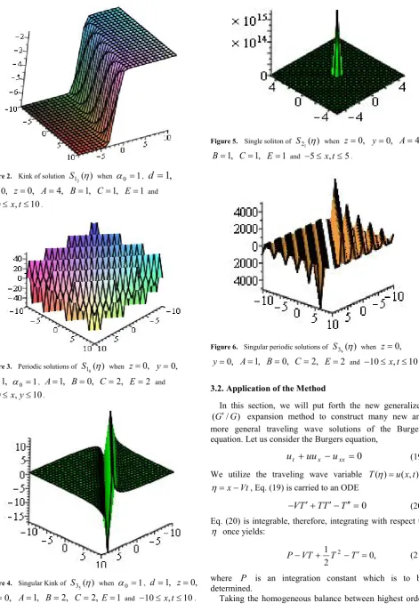
3.2.1. Table

Table 1. ComparisonbetweenKheiriandEbadi [36] solutions andoursolutions

Kheiri and Ebadi [36] solutions Obtained solutions

i. IfC₁=0 and u₁(

ξ

)=T₁(

η

), solutions Eq. (7)

becomes: )

2 4 coth(

1 ( ) 4 ( )

( 2 2

1

η

µ

λ

µ

λ

η

= − ± − −

T

i. If A=−1,

C

=

2

,

Ω=

λ

2 −4

µ

,

η

=−

ξ

,

µ

λ

α

2 2 4

0 +B+ d=± − then the solution is

) 2

4 coth(

1 ( ) 4 ( )

( 2 2

1

η

µ

λ

µ

λ

η

= − ± − −

T

ii. If C₁ =0 and u₃(

ξ

)=T₂₃(

η

), solutions Eq. (7)

becomes:

) 2 4 cot( 4

4 )

( 2 2 2

23

η

λ

µ

λ

µ

µ

λ

− − − × −

± = Φ T

ii. IfA=1,

C

=

0

,

Ω=

λ

2 −4

µ

,

µ

λ

α

2 2 4

0 −B− d=± − then the solution is

) 2 4 cot( 4

4 )

( 2 2 2

23

η

λ

µ

λ

µ

µ

λ

− − − × −

± = Φ T

iii. If ( ) ( )

5

2

2

ξ

T

η

u = , solution Eq. (7) becomes:

) (

2 ) (

2 1

2

25

η

C C

ξ

C T

+ =

iii. If A=1,

C

=

0

,

α

₀ −B−2d=0then the solution

is ( ) 2( )

2 1

2

25

η

_{C C}

ξ

C T

+ =

3.2.2. Results and Discussion

It is significant to state that one of our obtained solutions is in good agreement with the existing results which are shown in the Table 2. Beside this table, we obtain further new exact traveling wave solutions , , , , in this article, which have not been reported in the previous literature. In addition, the graphical representations of some obtained traveling wave solutions are shown in Figure 7 to Figure 10.

3.2.3. Graphical representations of the solution

[image:9.595.67.536.74.211.2]

The graphical illustrations of the solutions are depicted in the figures 7 to 10 with the aid of commercial software Maple 13.

Figure 7. Singular Kink of when

and .

Figure 8. Kink of solution when

and .

) (

2 2 η

T T2₄(η) T26(η)−T29(η)

) ( )

( ₉

1 1

1 η T η

T − T3₁(η)−T3₉(η)

) (

6

1

η

T

d

=

,1

α

₀ =1,

A

=

4

,

,

0

=

B

C

=

,1

E=1 −10≤x,t≤10

) (

2

1

η

T

α

₀ =1,

d

=

,1

,

4

=

[image:9.595.66.548.236.455.2] [image:9.595.74.558.587.739.2]

Figure 9. Periodic solutions of T1₃(η) when

α

0 =1,

d

=

,1

,

2

=

[image:10.595.303.556.75.452.2]

A

B

=

,1

C

=

4

,

E=1 and −10≤x,t≤10.

Figure 10. Singular Periodic solutions of ( )

8

3

η

T when

α

₀ =1,

,1

=

A

B

=

0

,

C

=

2

,

E=2 and −10≤x,t≤10.

4. Conclusion

Some new exact traveling wave solutions of the (3+1)-dimensional Zakharov-Kuznetsov equation and the Burgers equation are constructed in this article by applying the new generalized (G′/G) _{-expansion method. The}

traveling wave solutions are presented in terms of hyperbolic, trigonometric and rational functions. The performance of this method is trustworthy and gives many new solutions. Moreover, one of our obtained solutions are in good agreement with the existing results which validates our other solutions. Therefore, the new generalized (G′/G)

-expansion method can be further used to solve many nonlinear evolution equations which frequently arise in various scientific real time application fields.

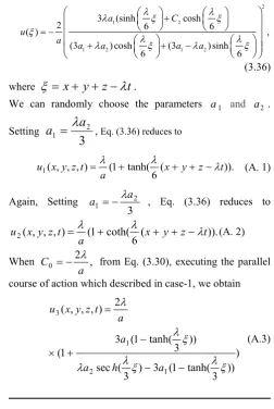
Appendix

Khan and Akbar [35] established exact solutions of the well-known (3+1)-dimensional ZK equation by using the modified simple equation method which are as follows:

2

1 2

1 2 1 2

3 (sinh cosh

2 6 6

( ) ,

(3 ) cosh (3 )sinh

6 6

a C

u

a _{a a a a}

λ λ

λ ξ ξ

ξ

λ λ

λ ξ λ ξ

+ = −

+ + −

     

   

 _{   } 

 

   

 _{   }

 _{   }

 

(3.36) where

ξ

=

x

+

y

+

z

−

λ

t

.

We can randomly choose the parameters a1 and a2.

Setting

3

2

1

a

a

=

λ

, Eq. (3.36) reduces to

)). (

6 tanh( 1 ( ) , , , (

1 x y z t _a x y z t

u =λ + λ + + −λ (A. 1)

Again, Setting

32

1 a

a =−

λ

, Eq. (3.36) reduces to

)). (

6 coth( 1 ( ) , , , (

2 x y z t _a x y z t

u =

λ

+

λ

+ + −

λ

(A. 2)

When ₀ 2 ,

a

C =−

λ

from Eq. (3.30), executing the parallel course of action which described in case-1, we obtain

) )) 3 tanh( 1 ( 3 ) 3 ( sec

)) 3 tanh( 1 ( 3 1

(

2 ) , , , (

1 2

1 3

ξ

λ

ξ

λ

λ

ξ

λ

λ

− − − +

×

=

a h

a

a a t z y x u

(A.3)

REFERENCES

[1] J. L. Hu, Explicit solutions to three nonlinear physical models. Phys. Lett. A, 287: 81-89, 2001.

[2] J. L. Hu, A new method for finding exact traveling wave solutions to nonlinear partial differential equations. Phys. Lett. A, 286: 175-179, 2001.

[3] A. M. Wazwaz, Partial Differential equations: Method and Applications, Taylor and Francis, 2002.

[4] V. B. Matveev and M.A. Salle, Darboux transformation and solitons, Springer, Berlin, 1991.

[5] M. R. Miura, Backlund transformation, Springer, Berlin, 1978.

[6] M. J. Ablowitz and P.A. Clarkson, Soliton, nonlinear evolution equations and inverse scattering method. Cambridge University Press, New York, 1991.

[7] J. S. Russell, Report on waves, in proceedings of the 14th Meeting of the British Association for the Advancement of Science, 1844.

[9] G. Xu, An elliptic equation method and its applications in nonlinear evolution equations. Chaos Solitons Fract., 29: 942-7, 2006.

[10] E. Yusufoglu and A. Bekir, Exact solution of coupled nonlinear evolution equations. Chaos solitons Fract. 37: 842-8, 2008.

[11] E. M. E. Zayed, H. A. Zedan and K. A. Gepreel, On the solitary wave solutions for nonlinear Euler equations. Appl. Anal., 83: 1101-32, 2004.

[12] J. H. He and X. H. Wu, Exp-function method for nonlinear wave equations. Chaos, Solitons and Fract., 30: 700-708, 2006.

[13] M. A. Akbar and N. H. M. Ali, Exp-function method for Duffing Equation and new solutions of (2+1) dimensional dispersive long wave equations. Prog. Appl. Math. 1(2): 30-42, 2011.

[14] M. A. Akbar and N. H. M. Ali,New Solitary and Periodic Solutions of Nonlinear Evolution Equation by Exp-function Method, World Appl. Sci. J., 17(12): 1603-1610, 2012. [15] H. Naher, A. F. Abdullah, and M. A. Akbar, New traveling

wave solutions of the higher dimensional nonlinear partial differential equation by the Exp-function method, J. Appl. Math., Article ID 575387, (2012) 14 pages. doi: 10.1155/2012/575387.

[16] M. M. Kabir, A. Khajeh, New explicit solutions for the Vakhnenko and a generalized form of the nonlinear heat conduction equations via Exp-function method, Int. J. Nonlinear Sci. Numer. Simul., 10(10): 1307–1318, 2009. [17] S. A. El-Wakil, M. A. Abdou, A. Hendi, New periodic wave

solutions via Exp-function method. Phys. Lett. A, 372: 830–840, 2008.

[18] A. M. Wazwaz, Exact solutions of compact and noncompact structures for the KP–BBM equation. Appl. Math. Comput., 169: 700–712, 2005.

[19] A. M. Wazwaz, The extended tanh method for the Zakharov Kuznetsov (ZK) equation, the modified ZK equation, and its generalized forms, Commun. Nonlinear Sci. Numer. Simul. 13(6): 1039, 2008.

[20] A. M. Wazwaz, A sine-cosine method for handle nonlinear wave equations. Appl. Math. Computer Modeling, 40: 499-508, 2004.

[21] A. H. Salas and C. A. Gomez, Application of the Cole-Hopf transformation for finding exact solutions to several forms of the seventh-order KdV equation, Mathematical Problems in Engineering, Art. ID 194329 (2010) 14 pages.

[22] M. L. Wang, X. Z. Li and J. Zhang, The

(

G

′

/

G

)

-expansion method and traveling wave solutions of nonlinear evolution equations in mathematical physics, Phys. Lett. A 372 (2008) 417-423.

[23] M. Song and Y. Ge, Application of the

( / )

G G

′

-expansion method to (3+1)-dimensional nonlinear evolution equations, Computers and Mathematics with Applications 60 (2010) 1220-1227.

[24] M. A. Akbar, N. H. M. Ali and E. M. E. Zayed, A generalized and improved (G′/G)-expansion method for nonlinear evolution equations, Math. Prob. Engr., Vol. 2012 (2012) 22 pages. doi: 10.1155/2012/459879.

[25] M. A. Akbar, N. H. M. Ali and S. T. Mohyud-Din, The alternative (G′/G) -expansion method with generalized Riccati equation: Application to fifth order (1+1)-dimensional Caudrey-Dodd-Gibbon equation, Int. J. Phys. Sci., 7(5) (2012) 743-752.

[26] M. A. Akbar, N. H. M. Ali and S. T. Mohyud-Din, Some new exact traveling wave solutions to the (3+1)-dimensional Kadomtsev-Petviashvili equation, World Appl. Sci. J., 16(11) (2012) 1551-1558.

[27] Q. Feng and B. Zheng, Traveling wave solutions for the fifth-order Sawada-Kotera equation and the general Gardner equation by (G′/G)-expansion method,Wseas Transaction on Mathematics, Issue 3 Vol. 9 (2010) ISSN: 1109-2769. [28] A. Bekir, Application of the (G′/G)-expansion method for

nonlinear evolution equations, Phys. Lett. A 372 (2008) 3400-3406.

[29] E. M. E. Zayed, The (G′/G)-expansion method and its applications to some nonlinear evolution equations in the mathematical physics, J. Appl. Math. Comput., 30 (2009) 89-103.

[30] S. Zhang, J. Tong and W. Wang, A generalized (G′/G)

-expansion method for the mKdV equation with variable coefficients, Phys. Lett. A 372 (2008) 2254-2257.

[31] A. J. M. Jawad, M. D. Petkovic and A. Biswas, Modified simple equation method for nonlinear evolution equations, Appl. Math. Comput., 217 (2010) 869-877.

[32] K. Khan, M. A. Akbar and M. N. Alam, Traveling wave solutions of the nonlinear Drinfel’d-Sokolov-Wilson equation and modified Benjamin-Bona-Mahony equations, J. Egyptian Math. Soc., DOI org/10.1016/j.joems.2013.04.010 (in press). [33] M. N. Alam, M. A. Akbar and S. T. Mohyud-Din, A novel

) /

(G′ G -expansion method and its application to the Boussinesq equation, Chin. Phys. B, Article ID 131006 (accepted for publication).

[34] H. Naher and F. A. Abdullah, New approach of (G′/G)

-expansion method and new approach of generalized

) /

(G′ G -expansion method for nonlinear evolution equation, AIP Advances 3, 032116 (2013); doi: 10. 1063/1.4794947.

[35] K. Khan and M. A. Akbar, Exact solutions of the (2+1)-dimensional cubic Klein-Gordon equation and the (3+1)-dimensional Zakharov-Kuznetsov equation using the modified simple equation method, Journal of Association of Arab Universities for basic and applied sciences (2013) xxx, xxx-xxx.

[36] H. Kheiri and G. Ebadi, Application of the (G′/G)