Statistical signal processing techniques for visual post production

(1)

Statistical Signal Processing Techniques

for Visual Post-Production

A dissertation submitted to the University of Dublin for the Degree of Doctor of Philosophy

François Pitié

Trinity College Dublin, May 2006

(2)

(3)

Abstract

Digital media post-production is an industry standard step in media creation. Now that issues of speed and physical storage have largely been rendered less problematic, the emphasis has shifted toward increasing levels of automation. This thesis makes several contributions in the domain of visual post-production in an attempt to bring advanced statistical digital signal processing techniques to bear on several key problem.

The problem of transfer of statistics is rst addressed. It transpires that this funda-mental process underlies several key problems in lm grading. This can be understood by considering an image as of features samples. Then texture or colour aspects can be described by the statistics of texture or colour samples. The rst and major problem is that of colour grading. In that process the colour of each lm frame has to be adjusted in order to match lighting and atmosphere throughout the shot. Consider a scene shot at midday and the same scene shot later in the afternoon, a typical procedure in movie production. The lm shot during the midday shoot will have a totally dierent look and feel than the afternoon shoot. In addition, brightness can change from frame to frame due to lm degradation, editing of dierent physical lm material and even uctuating lighting (e.g. uorescent). In all the cases the solution is to design an automated process that alters the distribution of colour and brightness of each frame in such a way that it balances across all shots. The thesis proposes a new mechanism for doing this based on the iterative matching of projections of the colour distribution on dierent set of colour axes. In addition, algorithms for robustness to grain artefacts artefacts caused by stretched histogram matching, and occlusion problems are also proposed.

The second part of the thesis deals with tracking of objects and contours. Both meth-ods proposed are founded on Bayesian grounds but adopt dierent optimisation strategies. Contour tracking is achieved by Bayesian Filtering exploiting a new prior that extracts local direction information from the image. Object tracking is achieved by a Viterbi al-gorithm that incorporates candidates for object position available in each frame. Both these tracking tools have implications for post-production. Contour tracking for rotoscop-ing is well established, but up till now incorporatrotoscop-ing edge information has been dicult. MCMC Bayesian lters have had great success for object tracking in recent times, but this thesis shows that given low level content knowledge it is possible to exploit deterministic strategies instead of MCMC and yield the same or better performance.

(4)

(5)

Declaration

I hereby declare that this thesis has not been submitted as an exercise for a degree at this or any other University and that it is entirely my own work.

I agree that the Library may lend or copy this thesis upon request.

Signed,

François Pitié

(6)

Acknowledgments

If you are reading this page, you are probably looking for your name, and you most likely deserve it, so thank you very much! Else I believe you are suering from compulsive insanity.

I would like to thank all former and present members of the Sigmedia group who have helped me over the years, and especially my PhD companions: the exhilarating Hugh DenmanAnil bless his thesis one dayfor his huge and generous help, and Dr. Francis Kelly because he's a man from Carlow and for all the good time in and outside the lab.

I wish to express my deep gratitude to my co-supervisor Dr. Rozenn Dahyot for the time and precious help she gave me. And of course, most of all, I would like to thank my supervisor Dr. Anil Kokaram for his patience and intelligence in deciphering my obscure drafts, the good atmosphere he instigates in the lab, his contagious motivation and, above all, his constant eorts and help over the last 3 years. Thanks Anil.

(7)

Chapter

1 Introduction

D

igital media technology is currently in an evolutionary stage. What is observed isthat technology domains like Computer Graphics, Computer Vision and Computer Vision are now converging. The convergence is patent in the research area where scientic papers can often be equivalently published in any of the conferences of these elds. The convergence is also reected in the industry where media applications are reciprocally bor-rowing core technologies. One emblematic example of this would be the recent integration of Industrial Light and Magicr_{, the special visual eects branch of Lucaslm Ltd., and} the gaming division LucasArtsr_.

There is thus a need to push this convergence further and bring recent advances in image processing to bear on key problems for media applications and especially for post-production. Digital media post-production is an industry standard step in media creation, which includes all stages of production between the actual recording and the complete lm or video. Now that issues of speed and physical storage have largely been rendered less problematic, the emphasis has shifted toward increasing levels of automation. Companies are already using image processing tools for simple automations. Only a few companies are however routinely using the most recent image processing advances. Examples of such companies are 2d3r_{with their feature-tracking engine Boujou, or The Foundry}r_{with their}

set of plug-ins Furnace.

(11)

CHAPTER 1. INTRODUCTION

1.1 Transfer of Statistics in Image Processing

The rst application considered in this work concerns a major problem in the post-production industry, which is to change the `look and feel' of the multitude of shots in such a way that they match the global atmosphere of the movie. Every aspect of the im-ages has to be carefully controlled: colour palettes, textures, form of the grain and so on. This activity of lm grading is currently xed by experienced artists who manipulate the frames by tuning parameters and painting what is possible to paint. Sometimes the aspect of the lm varies from frame to frame, like for instance in old footages where exposure time and lm stock ageing can be inconsistent. Then the brightness and colour aspect varies across frames and produces some annoying icker artefact. Similar uctuations also arise in modern footages if the sequence is a composition of dierent camera sources. In these cases, a similar restoration process needs to be performed to adjust the aspect of the frames throughout the shot.

One novel aspect of this thesis is to demonstrate that a statistical approach can help automating this painstaking process. Consider the colour aspect of an image: each picture can be represented by the set of its colour samples. The colour property or `feel' of a picture corresponds to the statistics of the colour samples. Then the grading the colour aspect of a frame can be done by transferring to the current frame the colour statistics of an example image that possesses the desired colour aspect.

The rst contribution of this thesis is to propose a method that transfers the complete statistics of the samples and not simply the mean and the variance as it is usually done. The method, described in chapter 2, is to nd a one-to-one mapping that transforms the original colour samples in a new set that exhibits the exact same propability density function (pdf) that the sample set of an example picture. With this method, it is easy to give the correct feel to an image sequence by simply providing a picture that has the wanted feel and then apply the corresponding mapping on each of the images. The rst application of the method is presented in chapter 3 and is a direct use of the method to the problem of recolouring of images by example. The second application, presented in chapter 4, is part of the larger process of the digital movie restoration and concerns the stabilisation of colour level uctuations across frames of a single shot or icker removal. The last chapter of this part studies ways of estimating the transfer of statistics in the presence of occlusions or missing data like blotches and dirt.

1.2 Probabilistic Tracking

(12)

mechanism. In the post-production industry however, objects are routinely manipulated. The objects are extracted using a combination of lming in a contrived environment (e.g. green-screen matting) or using manual delination of objects in each image frame. What is emerging is that for reliable segmentation, good enough to fool audiences, a combination of manual and automated tools are best. Two key operations are contour following to delineate an object in an image, and object tracking. Object tracking obviously has many applications outside of post-production.

The second main contribution of this thesis is to propose two probabilistic tracking algorithms that ease the burden of manual manipulation. Both methods proposed are founded on Bayesian grounds but adopt dierent optimisation strategies. The rst method is used for semi-automated contour delineationor rotoscoping. One recent technique called JetStream [Pér01] is a considerable advance on manual or semi-automatic tracing. The method, based on the use of Bayesian Filtering suers however from a lack of direction information in the image. The method proposed in chapter 6 exploits a new prior that extracts local direction information and so reworks the principle of density propagation for contour following.

The second method is a deterministic method used to track multiple objects in videos. A major diculty in tracking object is the dimension of the space of possible solutions. Popular stochastic methods like Particle Filters oer an attractive generic solution to this problem. These methods are simple to implement and can be easily scaled to any model complexity. It transpires however from a user point of view that deterministic methods are more suitable because reproduceable and predictable. The objective of this chapter is to show that it is often possible to simplify the object tracking problem in such way that it becomes tractable to provide a small set of deterministic position candidates and then use deterministic methods like Viterbi to track object among the reduced set of candidates.

1.3 Image Simplication

With both high-level information and low-level manipulations, it is now possible to develop media applications that would be content aware. This part explores the idea that objects of an images could be re-expressed in a dierent visual form that is not necessarily realistic but which conveys the same content. The aim is to develop representations that would have better viewability and that would be then transmitted or compressed easily.

Rendering non-photographic pictures has raised some interest in the computer graphic community, especially to design lters [Mig03] that simulate an artistic style. This concept is here pushed further by designing a non-photographic manipulation that focuses on the content of the images, whilst simplifying their representation.

(13)

non-parametric image models. The method consists in nding similar patches in the image and then replacing them by only one image patch that represents them all. This can be illustrated by considering an image sequence. An object can appear on several frames and presents slightly dierent appearances on these frames. Then replacing these object instances by a unique representation would still preserve the content while simplifying the video.

1.4 Thesis Outline

This thesis is thus divided into tree distinct parts. Part one covers chapters 2-5, part two covers chapters 6 & 7 and part tree the chapter 8. The part one treats the problem of transferring statistics from one image to another. Chapter 2 proposes a new method for doing so by transferring the actual pdf of image feature samples from one image to another. The method is applied to example-based image recolouring in chapter 3, and then extended to videos in chapter 4 for the restoration application of icker removal. Impatient (and reasonable) readers can rst focus on the description of the method in chapter 2 up to section 2.3, and then read the less mathematical application chapters 3 & 4. Chapter 5 considers ways of robustly estimating the transfer in the presence of outliers (e.g. content dierence). The second part, which covers chapter 6 & 7, presents two applications for probabilistic tracking. Finally chapter 8 concludes this thesis by presenting an implicit method for image simplication.

Chapter 2 proposes a novel method to estimate a continuous mapping that transfers one distribution to another. The distributions are possibly N-dimensional. The method

pro-posed is iterative, and its convergence is studied in the second part of the chapter.

Chapter 3 applies the method proposed in chapter 2 to the dicult problem of example-based image recolouring. The distribution transfer technique is used in conjunction with a post-processing algorithm that re-grains and protects the picture content. The results demonstrates the eectiveness of the method.

Chapter 4 applies the method proposed in chapter 2 to the problem of restoring image sequences degraded by brightness and colour uctuations. To treat this problem, referred to as icker removal, this chapter considers the possible variations of the mapping, temporally and spatially.

Chapter 5 considers the estimation of the mapping in situations where occlusions and missing data (outliers) pollute the original data samples (inliers). The chapter proposes two methods to separate outliers from inliers and then estimate the mapping.

(14)

Chapter 6 considers the problem of probabilistic tracking applied to the semi-automated delineation of object contours. This chapter considers the incorporation of a better di-rectional information in the JetStream algorithm [Pér01] and so reworks the principle of density propagation for contour following.

Chapter 7 considers shortcomings of MCMC approaches like Particle Filter methods as proposed in chapter 6 and points out that in many situations, it is possible to use a similar Bayesian framework but without having to resort to stochastic optimisation methods. The chapter illustrates this idea by presenting o-line multi-tracking applications.

Part III

Chapter 8 proposes an new implicit way of simplifying images by exploiting redundancy within images. The method aims at establishing statistics of pixel values according to their neighbourhood pixel values. Then by using Mean-Shift algorithm on the statistics pdfs results in an ltering that implicitly replaces similar objects by one instance of this object.

Contributions of this Thesis. This thesis oers new contributions which can be sum-marised by the following list.

• Transferring pdfs in N dimensions (chapter 2)

• Finding an optimised sequence of rotation matrices for theN-dimensional pdf

trans-fer (chapter 2)

• Transferring pdf in 1D in the presence of outliers (chapter 5)

• Generating randomly pdfs (chapter 2 and appendix A)

• Removing grain structures that appear after over-stretched mapping (chapter 3)

• Stabilising brightness uctuations in videos or Flicker Removal (chapter 4)

• Using GPU to speed up icker removal (chapter 4)

• Using edge direction information to track contours in pictures using particle lter

(chapter 6)

• Computing edge direction information (chapter 6)

• Using simple colour segmentation and deterministic algorithms (Viterbi) to track

players in videos (chapter 7)

• Establishing neighbourhood statistics to integrate an implicit prior in Mean-Shift

(15)

Part I

(16)

Chapter

2 Distribution Transfer

T

he principle of example-based rendering is probably the simplest and most eectiveapproach to rendering realistic images. The idea is to transform an original image in such a way that the resulting picture has the same `look and feel' as an example picture. One ecient method of realising this eect is to extract the image statistics of the example, and transfer them on the original image.

The notion of image statistics covers a wide range of properties. For instance, in the case of texture, the relevant image statistics are those pertaining to texture samples, and it is these statistics that are transferred to the original image. In the case of colour transfer, the image is expressed in terms of colour samples.

The recent breakthrough in texture synthesis and texture transfer [Efr99,Efr01,Her01] is one of the most signicant example of this idea. The texture transfer technique is based on a non-parametric approach, which consists simply in replacing the blocks in the original picture by the most similar blocks in a seed example texture. The resulting image consequently displays the same texture statistics as the target texture. As shown in gure 2.1, this technique gives impressive results, and suggests that achieving realistic rendering results relies on the transfer of real data statistics.

The original and example images can be represented as the two sets of feature samples

{ui}i≤M and {vi}i≤M0 respectively. The feature samples are possibly N-dimensional and

depend on the application. The problem is to nd a mappingtthat transforms the original

set{ui}i≤M into a new set{t(ui)}i≤M such that the statistics of the new data samples are

(17)

[image:17.595.162.458.408.683.2]

CHAPTER 2. DISTRIBUTION TRANSFER

Figure 2.1: Example of Texture Transfer (from [Her01]).

(18)

There is a wide range of possible approaches to the transfer of statistics. For example a linear mapping suces to match the means and the variances of the distributions. But if it is sought to transfer the actual probability density function (pdf) of the samples, the mapping becomes more complex. This latter problem will be referred to as the Distribution Transfer problem and is the subject of this chapter.

Distribution Transfer Problem. Consider a set ofM data samplesui. Denote byf the

continuous pdf of these samples. The problem is to nd an innitely dierentiable bijective mappingt:u→t(u) that transforms the original set {ui}i≤M into a new set {t(ui)}i≤M

such that the pdff0 of the transformed data samples is equal to a target continuous pdf g.

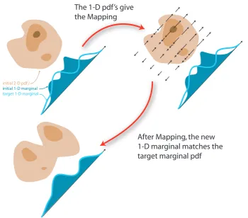
There are a few constraints on the transformation. Firstly, the dierentiable constraint is simply the mathematical expression that the transformation has to be smooth, in the sense that two feature samples that are similar in the original picture should still be loosely similar after transformation. Combined with the bijective constraint this means that the mapping has to be monotonic. This intuitive constraint has however some consequences of importance. For instance, under the monotonic constraint, it is impossible to allow swapping clusters of samples. Hence the operation in gure2.3 is not dierentiable, but simply at best piecewise dierentiable. Also the folding-like transformation described on the left of gure 2.4 is not allowable. This is because where the mapping folds (red arrows), multiple points have the same target, and this violates the bijective constraint. The allowable space of monotonic mappings encompasses transformations equivalent to deforming a rubber sheet.

Bearing these issues in mind, after a brief study of the linear case, this section proposes a solution to the distribution transfer. Although the concept of distribution transfer can provide a framework for thinking about texture manipulation, it will not necessarily yield in an ecient algorithm. However, in the case of colour transfer, it is clearly an attractive solution, as shown in the next chapter.

2.1 The Linear Case.

Consider at rst the case of a linear transformation as follows:

t(u) =Au+b (2.1)

The parameters of the transformationsA andb, can be derived by matching the rst and

second moments of both the original pdff and the target pdf g. Denote asµf andµg the

means off and g, and Σf and Σg as the covariance matrices:

(19)

1

2

3

1

3

2

Figure 2.3: Monotonous limitations: clusters cannot be swapped.

(20)

Figure 2.5: Matching 2 Normal distribu-tions. The assignment of axis numbers and directions should be consistent for both distributions.

The linear transformation is thus as follows:

t(u) = (Σg) 1

2(Σ_f)−

1

2(u−µ_f) +µ_g (2.4)

whereΣ

1 2

g is given by the Cholesky decomposition of Σg. Experience has shown however

that the Cholesky decomposition oers insucient control over the transformation. The preferred approach for this application is instead the singular value decomposition (SVD):

(Σf) = ETfDfEf

= D 1 2 fEf

2

(2.5)

(Σg) = ETgDgEg

= D 1 2 gEg

2

(2.6)

whereEf = [e1_f, . . . ,eN_f ]andEg = [e1g, . . . ,eNg ]are theNxN orthogonal matrices

contain-ing the eigenvectors of the covariance matrices. The diagonal matricesDf andDg contain

the eigenvalues corresponding to the eigenvectors inEf andEg. The nal transformation

is thus as follows:

t(u) =ET gD −1 2 g D 1 2

fEf(u−µf) +µg (2.7)

The additional control oered by the SVD method derives from the possibilities in or-dering the eigenvectors and choosing their direction (see gure2.5). For example, changing the sign of an eigenvector results in swapping the data samples from one side of the eigen-vector axis to the other side, which is not wanted. The idea is to preserve the content information by ordering the eigenvectors with respect to the magnitude of the correspond-ing eigenvalues and makcorrespond-ing sure that they do not point in opposite directions, i.e.

∀ i≤N , ei_fT

(21)

2.2 The General Non-Linear Case

2.2.1 The 1D case

Consider now the general distribution transfer problem where it is sought to transfer the actual target pdfg. If the data samples are of dimension 1, the distribution transfer

prob-lem has a very simple solution. The dierentiable mapping yields the following constraint which simply corresponds to a change of variables:

f(u)du=g(v)dv with t(u) =v (2.9)

Integrating both sides of the equality yields

Z u

f(u)du= Z t(u)

g(v)dv (2.10)

Using cumulative pdf notations F and G for f and g then yields the expression for the

mappingt,

∀u∈_R , t(u) =G−1(F(u)) (2.11)

where G−1(α) = inf{u|G(u)≥α}. The mapping can then easily be solved by using

discrete look-up tables.

2.2.2 Extending the 1D Case to Higher Dimensions

Extending the 1-dimensional case to higher dimensions is not trivial. The idea proposed here is to break down the problem into a succession of 1-Dimensional distribution transfer problems. Consider the use of the N-dimensional Radon Transform. It is widely

ac-knowledged that via the Radon Transform, anyN-dimensional function can be uniquely

described as a series of projections onto 1-dimensional axes [Weia]. In this case, the func-tion considered is aN-dimensional pdf, hence the Radon Transform projections result in

a series of 1-dimensional marginal pdfs. Intuitively then, operations on theN-dimensional

pdf should be possible through manipulations of the1-dimensional marginals.

Consider that after some sequence of such manipulations, all 1-dimensional marginals match the corresponding marginals of the target distribution. It then follows that, by nature of the Radon Transform, the transformed f, corresponding to the transformed

1-dimensional marginals, now matchesg.

(22)

2.2.3 Description of the Manipulation

The operation applied to the individual projection axes on the marginal distributions is naturally similar to that used in 1-dimension. Consider a particular axis denoted by its vector direction e∈ _RN_{. The projection of both pdfs} _f _and _g _{onto the axis} _e _{results in}

two 1-dimensional marginal pdfsfe andge. Using the 1-dimensional pdf transfer mapping

of the equation (2.11) yields a 1-dimensional mappingte along this axis:

∀u∈_R, te(u) =G_e−1(Fe(u)) (2.12)

For aN-dimensional sampleu= [u1,· · ·, uN]T, the projection of the sample on the axis is

given by the scalar producteT_u₌P

ieiui, and the corresponding displacement along the

axis is

u→u+ (te(eTu)−eTu)e (2.13)

After transformation, the projection f_e0 of the new distribution f0 is now identical to ge.

The manipulation is explained in gure2.6.

Considering that the operation can be done independently on orthogonal axes, the proposed manipulation consists in: choosing an orthogonal basis R = (e1,· · · ,eN) and

then applying the following mappingτ:

τ(u) =u+R



  

t1(eT1u)−eT1u

...

tN(eTNu)−e T

Nu



 

 (2.14)

whereti is the 1-dimensional pdf transfer mapping for the axisei.

The idea is that iterating this manipulation over dierent axes will result in a sequence of distributionsf(k)_{that hopefully converges to the target distribution}_g_{. The overall}

algo-rithm is described on a separate page and will be referred to as the Iterative Distribution Transfer (IDT) algorithm.

Although the theoretical study presented in section2.3does not provide yet a proof of convergence in all cases, the experimental results presented on gures2.7and 2.12clearly show that the method can be practically used as it is. Impatient readers can thus skip the rest of the chapter and resume their reading at chapter3which presents a direct application of the method to colour grading. Note however that the method can be substantially speeded up by using an optimised rotation sequence as proposed in section2.4.3.

2.3 Theoretical Convergence Study

(23)

The 1-D pdf’s give the Mapping

After Mapping, the new 1-D marginal matches the target marginal pdf

initial 2-D pdf f

initial 1-D marginal

[image:23.595.138.489.116.424.2]

target 1-D marginal

Figure 2.6: Illustration of the data manipulation, based on the 1-dimensional pdf transfer on one axis.

Algorithm 1 IDT method

1: Initialisation of the data set source u

k←0, u(0) ←u

2: repeat

3: for every rotated axisi, get the projections fi and gi

4: nd the 1D transformationti that matches the marginals fi intogi

5: remap the samplesu according to the 1D transformations:

u(k+1) =u(k)+R



 

t1(eT1u(k))−eT1u(k)

...

tN(eTNu(k))−e T

Nu(k)



 

6: k←k+ 1

7: until convergence on all marginals for every possible rotation 8: The nal one-to-one mappingT is given by: ∀ j ,uj 7→t(uj) =u(

∞)

(24)

50 100 150 200 250 50

100 150 200 250

50 100 150 200 250 50

100 150 200 250

50 100 150 200 250 50

100 150 200 250

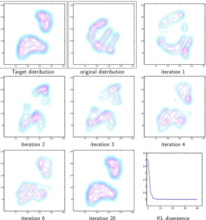
Target distribution original distribution iteration 1

50 100 150 200 250 50

100 150 200 250

50 100 150 200 250 50

100 150 200 250

50 100 150 200 250 50

100 150 200 250

iteration 2 iteration 3 iteration 4

50 100 150 200 250 50

100 150 200 250

50 100 150 200 250 50

100 150 200 250

0 10 20 30 40

0 0.5 1 1.5 2 2.5 3 3.5

[image:24.595.107.512.182.614.2]

iteration 6 iteration 20 KL divergence

(25)

at each iteration, it is possible to nd for any distributionf a dierentiable bijective

map-pingtf =τk◦ · · · ◦τ1that transformsf into the standard distributionN(0,idN). Consider

then the two dierentiable mappings tf and tg that transform f and g into N(0,idN).

Using the standard distributionN(0,idN)as a pivot results in the transformationt−g1◦tf,

which is a dierentiable bijective mapping that transforms f into g, and is therefore a

solution of the distribution transfer problem:

tf : f → N(0,idN)

tg : g→ N(0,idN)

∀u∈RN, t(u) =t−g1(tf(u))

(2.15)

The results of the convergence study in the next several paragraphs strongly suggest that the algorithm converges to the solution even if the target distribution is not the normal distribution. Figure2.7 shows an example illustrating the convergence of the process for 2-dimensional pdfs. Thus the method can also be used directly to nd a mapping between

f and g, without having to resort to the standard distribution as a pivot. The results of

the following chapters are based on this assumption and use the algorithm directly.

Theorem 1 (Isotropic Case). Letf be anN-dimensional pdf and denote byg the pdf of

the standard normal distributionN(0,idN). Consider the dierentiable transformationτk

that matches as in equation (2.14) the marginals of f to the projections ofg for a random

set of axes. Then the sequence dened by f(0) ₌_f _and _f(k+1) ₌_τ

k(f(k)) converges to the

target distribution: f(∞) =g.

Proof. Denote the original pdff and the target standard normal pdfg. For a particular

set of axes, denote f1,· · ·, fN the marginals off and g1,· · · , gN the marginals of g. The

standard distribution is isotropic and for all axes, it can be written as the product of its marginals: g = g1· · ·gN. The key of the proof is to show that the Kullback-Leibler

divergence decreases for any set of axes.

The Kullback-Leibler divergence, or relative entropy, is a quantity which measures the dierence between two probability distributions. It is computed as follows:

DKL(fkg) =

Z

u

f(u) ln

f(u) g(u)

du (2.16)

(26)

the KL divergence is always non-negative andDKL(p, q) is zero ip=q.

DKL(fkg) =

Z

u

f(u) ln

f(u) g(u)

du

= Z

u

f(u) ln

f(u) f1(u1)· · ·fN(uN)

du+ Z

u

f(u) ln

f1(u1)· · ·fN(uN)

g(u)

du

=DKL(fkf1· · ·fN) +

Z

u

f(u) ln

f1(u1)· · ·fN(uN)

g1(u1)· · ·gN(uN)

du

(2.17) Then by marginalising,

Z

u

f(u) ln

f1(ui)

gi(ui)

du= Z

u1

· · · Z

uN

f(u1,· · · , uN) ln

f1(ui)

gi(ui)

du1· · ·duN

= Z

ui

f(ui) ln

f1(ui)

gi(ui)

dui

=DKL(fikgi)

(2.18)

Eventually it follows that

DKL(fkg) =DKL(fkf1· · ·fN) + N

X

i=1

DKL(fikgi) (2.19)

Consider now that the mapping transformsf intof0 andf1· · ·fN intof10· · ·fN0 . It holds

forf0 that:

DKL(f0kg) =DKL(f0kf10· · ·f

0

N) +

N

X

i=1

DKL(fi0kgi) (2.20)

The transformation is such as for each axis i, f_i0 = gi, thus P_iN₌₁DKL(fi0kgi) = 0.

Also the KL divergence is left invariant by bijective transformation. This implies that

DKL(f0kf10· · ·fN0 ) = DKL(fkf1· · ·fN). Thus the KL dierence decreases at each

itera-tion by:

DKL(fkg)−DKL(f0kg) = N

X

i=1

DKL(fikgi)≥0 (2.21)

SinceDKL(fkg)is non-negative, it must have a limit. This implies that the KL divergence

on the marginalsDKL(fikgi) convergences to 0. Then, if a sucient number of dierent

axes is considered, all marginals of f converge to the marginals of g, and the Radon

transform off(k) converges to the Radon transform of g. The Radon transform admits a

(27)

2.4 Experimental Convergence Study

This section studies the convergence of the algorithm when the standard distribution is not used as a pivot. The study also considers the problem of nding sequence of axes that maximises the convergence speed of the algorithm.

To explore the convergence of the algorithm, a measure is needed to quantify how well the transformed distributionf(k) matches the target pdf g. Following the remarks of the

previous theorem, the Kullback Leibler divergence is used as such a measure. One simple experiment that could be used to assess the impact of axis sequences on convergence is simply to choose two particular datasets, use one as a target pdf and the other as a source pdf. Then for various axis sequences, the KL measure could be used to assess convergence as each iteration of the algorithm proceeds.

In order to provide more evidence for convergence though, it is sensible to use instead an ensemble of datasets which would cover the space of valid pdfs: in a sense then, a Monte Carlo method for assessment would be more useful. Therefore the problem is to generate at random, valid pdfs which then could be used to generate datasets for the application of the Distribution Transfer algorithm. Having done this, an ensemble average convergence or expected convergence measure could be obtained for a particular axis sequence using the mean KL divergence. This is as follows:

Ef,g(D(fkg))≈

1 Ns

X

i≤Ns

fi,gi∈P

D(fikgi) (2.22)

whereP denotes the space of the pdfs, thus each element p ∈ P is a pdf. Note that the

estimation of the KL divergence expectation is dependent on the way the pdfs are chosen: i.e. they should be well distributed over the space for the expectation not to be biased. Assuming no prior on the pdfs, they should be generated uniformly over the ensemble of all possible pdfs. This turns out to be an interesting problem, and is discussed in the following sections after some attention to the numerical estimation of the KL divergence.

With this measure of improvement, it is now possible to study the behaviour of dierent axis sequences. The last paragraph of this section presents an heuristic way of nding a sequence, which shows near optimal improvements.

2.4.1 Kullback-Leibler Divergence

(28)

−2 −1 0 1 2

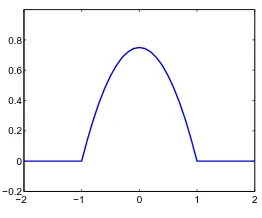
[image:28.595.244.375.102.211.2]

−0.2 0 0.2 0.4 0.6 0.8

Figure 2.8: Epanechnikov Kernel. This is the function K(u) = (3/4)(1− kuk2₎ _for

−1<kuk<1 and zero for kuk outside that range.

the underlying pdfs as follows:

D(f kg) = 1 M M X i=1 ln   P jK _u

i−uj

hi

P

jK

_u

i−vj

hi



 (2.23)

where K is the Epanechnikov kernel (see gure 2.8). To account for the sparseness of

samples, it is crucial to use a variable bandwidth approach. Typically, for a sampleui, the

bandwidthhi increases if with the sparseness of the samples around ui. A clear outline of

the bandwidth selection is available in [Com01], and that is used here. A major aspect of the experiment is that the KL divergence has to be non-negative. This is indeed observed in numerical results (see gure 2.7), but not for any choice of bandwidth values. To counterbalance this sensitivity, the pdf is over-smoothed by taking larger values of kernel bandwidths. The resulting KL divergence measure is under-evaluated since both estimated pdfs are more uniform. Another consequence is that the convergence speed measured on the gure2.12is actually slower than the true one.

2.4.2 Experimental Datasets: Sampling PDFs

As discussed above, measuring the KL divergence on a single example is of course insu-cient to infer any useful information. The estimation of the average KL measure requires to evaluate the KL divergence for a large number of datasets (say at least 100), and it is thus necessary to nd a way of generating these pdfs. In this study, there is no prior made on the distributions. This means that the pdfs of the datasets have to be generated in a uniform `random' way. Once a pdf has been generated, the set of N-dimensional data

samples is obtained by sampling directly from the newly generated pdf.

(29)

estimate the KL divergence. But since the KL estimation already over-smooths the pdf estimation, this does not present a major issue. The kernel approximation is as follows:

q(u) = 1 k k X i=1 qi hN i K

u−µi hi

(2.24)

whereNis the dimension of the pdf space,µiare the centres of the kernels,hithe associated

bandwidth, and (qi)i≤k a set weights such that Pik=1qi = 1 and qi ≥ 0. Since no prior

information is available on the pdf, it is standard to consider a at prior for the centres and the standard deviations:

p(µi) ∝ 1 (2.25)

p(hi) ∝

1

hi (2.26)

The centres µi are thus generated by sampling from a from a simple uniform spatial

distribution on the region of interest, or data range, Ω: µi ∼ U(Ω). Since the prior

p(hi) on the bandwidths is not a proper prior (it does not integrate to 1), the range of

values for the bandwidth is restricted from 1% to 100% of the data range. For instance, with a data range of[0; 255], the diametre is 256, and the bandwidth can go from 2.56 to

256. As seen in gure1, the lower bound of the bandwith values controls the smoothness of the generated pdf.

It still remains to generate the weights(qi)i≤k. Since(qi)i≤k is non-negative and sums

up to 1, this is the pdf of a random variable havingk possible states, and will be referred

to as ak-state pdf. It is shown in the appendixA.1a method for generating a k-state pdf

presents. The method is to generatekexponential random variables(z1, z2,· · · , zk). Then

the distribution of the vectors

1 z1+. . .+zk

    z1 ... zk     (2.27)

is uniform over the k-state pdf space (see appendix A.1 for a proof). Now that all the

parametersµi, hi, qi are known, it is possible to generate valid pdfs uniformly over the pdf

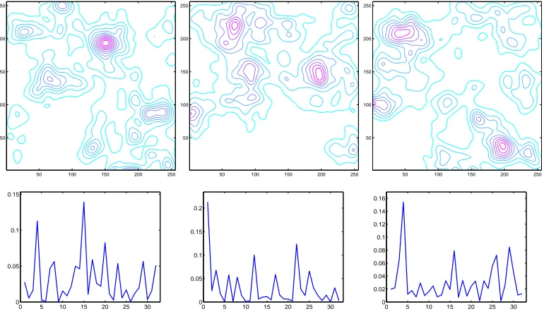
space. The overall method is summarised by Algorithm2, and examples of 1-dimensional and 2-dimensional pdfs generated by the method are displayed on gure2.10.

2.4.3 Results and Choice of Axis Sequence

(30)

0 50 100 150 200 250

0 0.1 0.2 0.3 0.4 0.5 0.6 0.7

0 50 100 150 200 250

[image:30.595.120.505.442.666.2]

0 0.005 0.01 0.015 0.02

Figure 2.9: Generating a pdf. The pdf here is modelled by a sum of 4 kernel functions. On the left, the positions of the vertical bars correspond to the po-sitions of centroids, the heights of the bars to the weight and the width of the overhead horizontal line to the size of the bandwidth (these values are generated by algorithm 2). The resulting pdf using gaussian kernels is presented on the right.

50 100 150 200 250 50

100 150 200 250

50 100 150 200 250 50

100 150 200 250

50 100 150 200 250 50

100 150 200 250

0 5 10 15 20 25 30 0

0.05 0.1 0.15

0 5 10 15 20 25 30 0

0.05 0.1 0.15 0.2

0 5 10 15 20 25 30 0 0.02 0.04 0.06 0.08 0.1 0.12 0.14 0.16

(31)

Algorithm 2 Sampling pdfs randomly

The pdf is modelled by a sum of kernel functions

q(u) = 1 k

k

X

i=1

qi

hN_i K

u−µi hi

(2.28)

The parameters are sampled as follows:

p(µi) ∝ 1 µi ∈Ω (2.29)

p(hi) ∝ 1/hi (2.30)

qi =

ei

e1+. . .+ek with

p(ei)∝exp(−ei) (2.31)

min bandwidth = 1% min bandwidth = 3% min bandwidth = 5%

(32)

100 dierent pdfs. Figure 2.12 shows the evolution of the KL divergence for a random selection of axis set sequences, with both random initial and target distributions. This result strongly suggest that the convergence occurs when the target distribution is not the standard distribution but any distribution. This in an important result since it gives ground to use the IDT algorithm, without having to use the standard distribution as a pivot.

Taking a random selection of orthogonal bases seems to be sucient to obtain con-vergence, however it is shown hereafter, that a better choice of axis sequence can still substantially improve the convergence speed. This can be understood by considering that random axes are probably correlated. Figure 2.13 shows that for small dimensions, two random vectors are more likely to be aligned than orthogonal. This result can be extended to the distance between orthogonal bases: two random orthogonal basis are more likely to be similar in dimension 2 than in dimension 10. Figure 2.14 conrms this intuition. The gure displays the average KL divergence after two iterations of the algorithm for 2D pdfs. At iteration 1, a xed set of axes is chosen, thus the plot shows the evolution of the KL divergence depending on the choice of axes at iteration 2. The graph clearly shows that the KL improvement depends on the correlation between axes.

Intuitively then, an interesting heuristic would be to consider a sequence of rotations that maximises the distances between the current axis set at iterationkand the previous

axis sets. Dene the distance between two axes by

d(e1,e2) = min(ke1−e2k2,ke1+e2k2) (2.32)

withe1 ande2 the supporting axis vectors. To nd axes that are far apart, one solution is

to maximise the distancesd(e1,e2). This turns out to a numerically unstable solution. A

better formulation is to consider instead the minimisation of the potential1/(1 +d(e1,e2))

and then to express that distances should be far appart with the following recursion:

e1_k₊₁,· · ·,eN_k₊₁

= arg min

[e1_,_···_,_eN_]

   k X l=1 N X i=1 N X j=1 1

1 +d(ej_l,ei₎

 



(2.33)

with the constraint that the bases are orthogonal. This minimisation problem can be numerically simulated under MATLAB using standard minimisation algorithms. The con-straint of normalisationkek= 1can be avoided by taking hyperspherical coordinates [Wik].

The orthogonality of the base can be obtained using Gram-Schmidt orthogonalisation. The resulting rst bases for dimension 2 and 3 are given in appendix tablesA.1andA.2. Note that since the algorithm is iterative, it is not crucial to require high accuracy in the esti-mation of the bases. The code used to nd the bases is available on [Pit06].

(33)

is sought, is optimal on average over the couple of pdfs. Note that other strategies could be explored, like nding the optimal sequence of axis for a particular couple of distributions.

2.5 Conclusion

Transferring statistics from one image to another is a non-trivial task if the samples are multidimensional. The method which is proposed is attractive since it fast and the results strongly suggests that the it converges for any continuous distribution. Note as well that the implementation of the method is straightforward. The following chapters explores two applications of this technique that work on the colour aspect of images.

It has been discovered towards the end of this PhD. that the problem exposed in this chapter shares similitude with the problem of Mass Transfer. More details about this problem can be found in [Eva99]. The original problem, rst proposed by Monge in the 1780's, is to minimise the amount of work needed to move a pile of soil to an excavation. Using modern notations, the pile and excavation correspond to two pdfsf and g, and the

problem is equivalent to nd a bijective mapping, that transformsf intog. The problem

(34)

0 2 4 6 8 10 12

0 0.2 0.4 0.6 0.8 1 1.2 1.4

0 2 4 6 8 10 12

0 0.1 0.2 0.3 0.4 0.5 0.6 0.7 0.8

average KL in 2D average KL, in 3D

Figure 2.12: Averaged evolution of the Kullback Leibler divergence for 100 sim-ulations with both random initial distribution and target distribution. Rotations are taken randomly. It transpires from the results that convergence occurs for any distribution.

0 0.2 0.4 0.6 0.8 1 0 0.005 0.01 0.015 0.02 0.025 0.03 0.035 0.04 0.045 n=2 n=3 n=4 n=6 n=10 n=17 n=30

0 0.1 0.2 0.3 0.4 0.5

0 0.05 0.1 0.15 0.2 0.25 0.3 0.35 0.4 n=10 n=2 n=6 n=4 n=3

(a)- distance between vectors (a)- distance between matrices

Figure 2.13: In (a): experimental measure of the average distance between two unit vectors in function of the space dimension. The distance between two vectorsu and v is given byd(u, v) = min(ku−vk2,ku+vk2). The average distance

clearly increases with the dimensionality, which in other words shows that random vectors are likely to be nearly orthogonal in high dimensions. The gure (b) extends the results to the distance between matrices of space transformation. The distance between two matrices A= [a1,· · ·, an] and B = [b1,· · · , bn] is given

by d(A, B) = mini,jd(ai, bj). As in (a), the average distance clearly increases

(35)

0 PI/8 PI/4 3PI/8 PI/2

0.2 0.3 0.4 0.5 0.6 0.7

0 PI/8 PI/4 3PI/8 PI/2

0.12 0.14 0.16 0.18 0.2 0.22 0.24

(a) -k= 2 (b) -k= 3

Figure 2.14: Average KL divergence to target distribution in function of the rota-tion sequence. The distriburota-tions are 2D and the rotarota-tion matrix can be represented by a single angle α between 0 andπ/2. On the left, after one iteration atα = 0.

The best rotation is for α =π/4, which corresponds to the less correlated axes.

On the right, after α = 0, π/4. The best new rotation occurs around α = 3π/8

and π/8.

0 2 4 6 8 10 12 14

−6 −5 −4 −3 −2 −1 0 1 Iteration Number Log 2 (KL)

0 2 4 6 8 10 12 14

Iterations Nb − Random Rotations

Iteration Number − Optimized Rotations

Figure 2.15: Optimised Rotation Sequence Speed Up for N = 2. On the left, the

averaged evolution of the log Kullback Leibler divergence for 100 simulation for both a random sequence of rotations and an optimised sequence of rotations. On the right, the correspondence between iteration numbers for both strategies. It requires in average 53% less iterations forN = 2when using an optimized rotation

(36)

0 2 4 6 8 10

−5 −4.5 −4 −3.5 −3 −2.5 −2 −1.5 −1 −0.5 0

Iteration Number

Log

2

(KL)

0 2 4 6 8 10

Iteration Nb − Random Rotations

Iteration Number − Optimized Rotations

Figure 2.16: Optimised Rotation Sequence Speed Up for N = 3. On the left, the

averaged evolution of the log Kullback Leibler divergence for 100 simulation for both a random sequence of rotations and an optimised sequence of rotations. On the right, the correspondence between iteration numbers for both strategies. It requires in average 33% less iterations forN = 3when using an optimized rotation

(37)

Chapter

3 Image re-Colouring

T

here are a wide range of applications for the notion of exact transfer of distribution formultidimensional datasets. This chapter considers the dicult problem of example-based re-colouring [Rei01]. The idea of example-example-based re-colouring is illustrated by the picture below. The `mountain' picture is required to be transformed so that its colours match the palette of the `plain' image, regardless of the content of the pictures.

Original Colour Palette re-Coloured Image

Consider the two pictures as two sets of three dimensional colour pixels. A way of treating the re-colouring problem would be to nd a one-to-one colour mapping that is applied for every pixel in the original image. For example in the diagram above, every white pixel is re-coloured in blue. Then the new picture is identical in every aspects to the original picture, except that the picture now exhibits the same colour pdf, or palette, as the target picture.

Estimating the mapping can be dicult, but if it is supposed to be continuous, a so-lution is had through the distribution transfer techniques for three dimensional datasets

(38)

CHAPTER 3. IMAGE RE-COLOURING

as discussed in previous chapter. Thus this chapter examines the application of the distri-bution transfer techniques in the context of image re-colouring. Note that the continuous assumption only transcribes the intuitive idea that two colours that are perceptually sim-ilar should be also mapped to simsim-ilar colours. This also implies that colours cannot be swapped. For instance, it is impossible to map a white to black and a black to white in the same picture. Figure 3.1 illustrates this contrast limitation. To realise a successful transfer, the sky of the picture should be segmented and treated separately.

Re-colouring picture with another has many applications in Computer Vision and in the Post-Production eld. In digital restoration [Pap00] the idea is to recolour paintings that have been faded by smoke, dust etc. The process can also be used for colour im-age equalisation for scientic data visualisation [Pic03] or simply useful for non-realistic rendering.

A major problem in the post production industry is matching the colour between dierent shots possibly taken at dierent times in the day. This process is part of the large activity of lm grading in which the lm material is digitally manipulated to have consistent grain and colour. The term colour grading will be used specically to refer to the matching of colour. Colour grading is important because shots taken at dierent times under natural light can have a substantially dierent `feel' due to even slight changes in lighting. Currently these are xed by experienced artists who manually match the colour between frames by tuning parameters. This is delicate task since the change in lighting conditions induces a very complex change of illumination. The method presented in this chapter however succeeds in automating this painstaking process even when the lighting conditions have dramatically changed as shown in gure3.6.

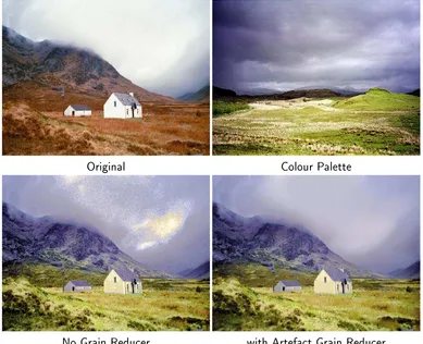
The one-to-one colour mapping to the original picture makes the transformed picture have the same `feel' of the picture example but it might also produce some grain artefacts on parts of the picture. This can be understood by considering a mapping from a low dynamic range to a high dynamic range. The resulting mapping is stretched and thus enhances the noise level of the picture, which makes the transformed picture appear grainy. The second step in colour grading is therefore to reduce this artefact. The method proposed is to use a variational approach to preserve the gradient of the original while preserving also the colour transfer characteristic. Preserving the gradient of the original picture especially protects the at areas and more generally results in preserving the nature of the lm grain/noise as in the original image.

(39)

3.1 Related Works

Transfer of Colour Statistics. One popular method proposed by Reinhard [Rei01] matches the mean and variance of the target image to the source image. The transfer of statistics is performed separately on each channel. Since the RGB colour space is highly correlated, the transfer is done in another colourspacelαβ. This colourspace has been proposed in an

eort to account for for human-perception of colour [Rud98]. But the method is limited to linear transformations. In fact, the motion picture industry employs routinely non-linear colour grading techniques. Hence, in a practical situation, some example-based recolouring scenarios actually require non-linear colour mapping. Figure3.2shows exactly this problem and the method fails to transfer any useful statistics.

The problem of nding a non-linear colour mapping is addressed in particular in [Pic03] for colour equalisation (c.f. grayscale histogram equalisation). That work proposes to deform tessellation meshes in the colour space to t to the 3D histogram of a uniform distribution. This method can be seen as being related to warping theory which is explicitly used in [Luc01] where the transfer of the 2D chromatic space is performed directly by using a 2D-bi-quadratic warping. Without having to invoke image warping, a natural extension of the 1D case is to treat the mapping via linear programming and the popular Earth-Mover distance [Mor03]. The major disadvantage of the method is that 1) the mapping is not continuous and 2) pixels of same colours may be mapped to pixels of dierent colours, which require random selection. Furthermore the computational cost becomes intractable if a very ne clustering of the colour space is desired.

Dealing with Content Variations. One important aspect of the colour transfer problem is the change of content between the two pictures. Consider a pair of images which are of landscapes but in one picture the sky covers a larger area than the other. When transferring the colour from one picture to the other therefore, the sky colour may be applied also to parts of the scenery on the ground in the other. This is because all colour transfer algorithms are sensitive to variations in the areas of the image occupied by the same colour, they risk overstretching the colour mappings and thus producing unbelievable renderings. To deal with this issue a simple solution (presented in [Rei01] ) is to manually select swatches in both pictures and thus associate colour clusters corresponding to the same content. This is tantamount to performing manual image segmentation, and is simply impractical for a large variety of images, and certainly for sequences of images.

(40)

Original Colour Palette Resulting Transfer

Figure 3.1: Issues of the Continuous Assumption for Colour Transfer. The Cam-panile appears clearer than the sky in the original picture, and darker than the sky in the target picture. This contrast inversion can not be handled correctly by continuous transfer. Even if the result image has the same colour statistics than the target image, the transfer is clearly not the one wanted. Note that the white of the Campanile comes from the white of the target sky.

Original Colour Palette Reinhard Results

(41)

categories, derived from psycho-physiological studies (red, blue, pink . . . ). The colour transfer ensures for instance that blue-ish pixels remain blue-ish pixels. This gives a more natural transformation. The disadvantage is that it limits the range of possible colour transfers.

Novelty. Using the distribution transfer method for the example-based recolouring problem can x many of the shortcomings of previous eorts in this area. Firstly, it is computa-tionally attractive as it uses just 1D pdf matching in an iterative scheme. Secondly, the method is completely non-parametric and is very eective at matching arbitrary colour distributions. Thirdly, the proposed method for reducing grain artefact results in high quality picture.

3.2 Reducing Grain Noise Artefacts

The colour mapping to the original picture transfers correctly the target colour palette to the original picture but it might also produce some grain artefacts as shown in gure 3.2

and 3.5. When the content diers, or when the dynamic range of both pictures are too dierent, the resulting mapping function can be stretched on some parts (see gure3.2-e), and thus enhances the noise level (see gure3.2-c). This can be understood by taking the simple example of a linear transformationt of the original pictureI: t(I) =a I+b. The

overall variance of the resulting picture is changed to var{t(I)}=a2 var{I}. This means

that a greater stretching (a >1) produces a greater noise.

The solution proposed here to reduce the grain is to run a post-processing algorithm that forces the level of noise to remain the same. The idea is to adjust the gradient eld of the picture result so that it matches the gradient eld of the original picture. If the gradient elds of both pictures are similar, the level of noise will be the same. Matching the gradient of a picture has been addressed in dierent computer vision applications like high dynamic range compression [Fat02]; the value of this idea has been thoroughly demonstrated by Pérez et al. in [Pér03]. The manipulation of gradient can be eciently solved using a variational approach. The problem here is slightly dierent, since re-colouring also implies changing the contrast levels. Thus the new gradient eld should only loosely match the original gradient eld.

Denote I(x, y) the 3-dimensional original colour picture. To simplify the coordinates

are omitted in the expressions andI,J,ψ,φ, etc. actually refer to I(x, y),J(x, y),ψ(x, y)

and φ(x, y). Let t : I → t(I) be the colour transformation. The problem is to nd a

modied imageJ of the mapped picturet(I) that minimises on the whole picture rangeΩ

min

J

Z Z

Ω

φ· ||∇J − ∇I||2₊_ψ_{· ||J} ₋_t₍_I₎_||2_d_x_d_y _(3.1)

with Neumann boundaries condition ∇J|∂Ω = ∇I|∂Ω so that the gradient of J matches

(42)

(a)-Original (b)-Target

0 50 100 150 200 250 0

50 100 150 200 250

[image:42.595.117.493.251.481.2]

(c)-Recoloured (d)-denoised (e) mapping

(43)

gradient to be preserved. The term ||J −t(I)||2 _{ensures that the colours remain close to}

the target picture and thus protects the contrast changes. Without||J−t(I)||2_{, a solution}

of equation (3.1) will be actually the original pictureI.

The weight eldsφ(x, y)andψ(x, y)aect the importance of both terms. Many choices

are possible for φ and ψ, and the following study could be easily be changed, depending

on the specications of the problem.

The weight eldφhas been here chosen to emphasise that only at areas have to remain

at but that gradient can change at object borders:

φ(x, y) = 30

1 + 10||∇I|| (3.2)

The weight eldψ accounts for the possible stretching of the transformationt. Where ∇t

is big, the grain becomes more visible:

ψ(x, y) =  



2/(1 +||(∇t)(I)||) if ||∇I||>5

||∇I||/5 if ||∇I|| ≤5 (3.3)

where(∇t)(I) is the gradient oft for the colourI and thus refers to the colour stretching.

The case ||∇I|| ≤ 5 is necessary to re-enforce that at areas remains at. While the

gradient oftis easy to estimate for grayscale pictures, it might be more dicult to obtain

for colour mappings. The eld can then be changed into:

ψ(x, y) =  



1 if ||∇I||>5

||∇I||/5 if ||∇I|| ≤5 (3.4)

Numerical Solution. The minimisation problem in equation (3.1) can be solved using the variational principle which states that the integral must satisfy the Euler-Lagrange equation: ∂F ∂J − d dx ∂F ∂Jx − d dy ∂F ∂Jy

= 0 (3.5)

where

F(J,∇J) =φ· ||∇J− ∇I||2+ψ· ||J−t(I)||2 (3.6)

from which the following can be derived:

φ·J −div (ψ· ∇J) =φ·t(I)−div (ψ· ∇I) (3.7)

This is an elliptic partial dierential equation. The expression div (ψ· ∇I) at pixel x = (x, y) can be approximated using standard nite dierences [Wei98] by:

div (ψ· ∇I) (x)≈ X xn∈Nx

ψxn+ψx

(44)

whereNx corresponds to the four neighbouring pixels of x. Using this in equation (3.7)

yields a linear system as follows:

a1(x, y)J(x, y−1) +a2(x, y)J(x, y+ 1) +a3(x, y)J(x−1, y) +a4(x, y)J(x+ 1, y)

+a5(x, y)J(x, y) =a6(x, y)

(3.9)

with

a1(x, y) = −

ψ(x, y−1) +ψ(x, y) 2

a2(x, y) = −

ψ(x, y+ 1) +ψ(x, y) 2

a3(x, y) = −

ψ(x−1, y) +ψ(x, y) 2

a4(x, y) = −

ψ(x+ 1, y) +ψ(x, y) 2

a5(x, y) = 1 2

4ψ(x, y) +ψ(x, y−1) +ψ(x, y+ 1) +ψ(x−1, y) +ψ(x+ 1, y)

+φ(x, y)

a6(x, y) = 1 2

ψ(x, y) +ψ(x, y−1))(I(x, y−1)−I(x, y))

+ (ψ(x, y) +ψ(x, y+ 1)(I(x, y+ 1)−I(x, y))

+ (ψ(x, y) +ψ(x−1, y)(I(x−1, y)−I(x, y))

+ (ψ(x, y) +ψ(x+ 1, y)(I(x+ 1, y)−I(x, y))

+φ(x, y)I(x, y)

The system can be solved by standard iterative methods like SOR, Gauss-Seidel with multigrid approach. Implementations of these numerical solvers are widely available and one can refer for instance to the Numerical Recipes [Pre92]. The main step of these methods is to solve iteratively for J(x, y). Note that J(x, y) and ai(x, y) are of dimension 3, but

that each colour component can be treated independently. For instance, the iteration for the red component eld is of the form

J_R(k+1)(x, y) = 1 aR₅(x, y)

aR₅(x, y)−a₁R(x, y)J_R(k)(x, y−1)−aR₂(x, y)J_R(k)(x, y+ 1)

−aR₃(x, y)J_R(k)(x−1, y)−a₄R(x, y)J_R(k)(x+ 1, y)

(3.10)

whereJ_R(k)(x, y) is the result in the red component at the kth iteration.

3.3 Results

(45)

column.

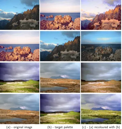
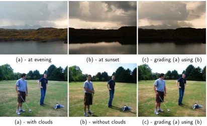
Examples of Colour Grading for matching lighting conditions are presented in3.6. On the rst row, the colour properties of the sunset are used to synthesise the `evening' scene depicted at sunset. On the second row, the colour grading allows correction of the change of lighting conditions induced by clouds. Even when using the grain artefact reducer, an unavoidable limitation of colour grading is the clipping of the colour data: saturated areas cannot be retrieved (for instance the sky on the golf image cannot be recovered). A general rule is to match pictures from higher to lower range dynamics.

The gure 3.7 displays examples of colour restoration of faded movies. The idea is similar to colour grading as the idea is to recreate dierent atmospheres. The target pictures used for recreating the atmosphere are on the second row.

3.4 Conclusion

(46)

[image:46.595.108.520.183.619.2]

(a) - original image (b) - target palette (c) - (a) recoloured with (b)

(47)

Original Colour Palette

[image:47.595.117.506.241.557.2]

No Grain Reducer with Artefact Grain Reducer

(48)

(a) - at evening (b) - at sunset (c) - grading (a) using (b)

[image:48.595.106.519.115.366.2]

(a) - with clouds (b) - without clouds (c) - grading (a) using (b)

Figure 3.6: Examples of Colour Grading for matching lighting conditions. On the rst row, the colour properties of the sunset are used to synthesise the `evening' scene depicted at sunset. On the second row, the colour grading allows to correct the change of lighting conditions induced by clouds.

Original Frame 70's atmosphere pub atmosphere

Original Frame Original 70's atmosphere Original pub atmosphere

[image:48.595.119.506.482.672.2]

(49)

Chapter

4 Stabilisation of Brightness Fluctuations in Image Sequences

W

hile in re-Colouring images the target colour palette is known, there exists a numberof scenarios where the target palette is a priori unknown. Consider an image sequence, where colour and brightness levels uctuate for each frame of the sequence. The problem is to align these levels in order to remove the uctuations. The underlying ground-truth target palette is unknown and the problem comes down in rst place to estimate the target palette. Most frequently uctuations also present some spatial correlation, which need also to be accounted for. This chapter proposes a solution to this problem by extending the ideas developed in the previous chapters to include both temporal and spatial considerations.

Instances of Brightness Fluctuations. Random uctuation in the observed brightness of recorded image sequences, also called icker, occur in a variety of situations. The most commonly consumer observed instance of icker is in archived lm and video (see gure4.1and 4.2, see also examples of videos in [Pit02]). It is caused by the degradation of the medium (ageing of the lm stock), varying exposure times, or curious eects of poor standards conversion. Varying exposure time is common to hand-cranked footages, but happens too with mechanised cameras in early lms or most recently with personal 8mm. Remarkably icker often aects modern lm and video media if the lighting conditions are poor, as in submarines surveillance, or when the transfer from lm to video (telecine) is not properly done.

The icker artefact is still an actual issue, even with the use of digital cameras. Consider

(50)

CHAPTER 4. FLICKER REMOVAL

for instance the popular Inbetweening special eect used in The Matrix (1999). This special eect is based on the interpolation of images coming from multiple cameras shouting with dierent angle the same scene. Unfortunately, the brightness levels of the pictures are sometimes misaligned. This is due to dierent camera behaviour or lighting conditions due to camera orientation, even if video cameras have been previously calibrated using radiometric calibration routines. Figure4.3shows this radiometric calibration issue for an outdoor footage.

Consequences. The presence of icker is often praised by lm enthusiasts as an essential aesthetic element of the lm experience. Unfortunately people with medical conditions or simply high sensitivity to ickering can suer eye strain and even headaches while watching such movies. This results of course in much discomfort and pain.

From an image processing point of view, the presence of icker has also a detrimental eect on many applications since it breaks the common assumption that object brightness is constant over the frames (this is the so-called brightness constancy). For instance, motion estimation [Lai99, Jin01] or any other image matching algorithms fail in presence of icker as they try to match brightness levels of two pictures.

Brightness uctuations have also dramatic consequences on the video compressibility. The icker reduces the redundancy between frames and hence increases the bandwidth of transmitted sequences. This is particularly a problem for Digital Television or broadcasting of video content over the Internet.

Organisation of the Chapter. This chapter proposes therefore to stabilise these uctua-tions in image sequences. Dealing with the problem of icker requires some attempt to model or measure the uctuation between frames (the estimation process), and then to remove this uctuation in some way (the correction process). The core of the model and its estimation process rely on the re-colouring technique exposed in the previous chapter. After an exposition of related works in the area, the following sections examine how to integrate spatial and temporal considerations to distribution transfer techniques, in order to establish a generic icker removal framework. In addition, this chapter proposes a novel implementation based on general purpose PC graphics hardware. The results show that it is possible to cope with a wide range of icker eect. The section4.5presents results show-ing the eect of icker on MPEG4 compression of dierent kinds of sequences includshow-ing multi-view camera sequences, and the improvement in bandwidth usage with the proposed icker reduction method.