OPTIMAL REPLENISHMENT POLICY FOR NON INSTANTANEOUS DETERIORATING ITEMS WITH IMPRECISE DEMAND RATE

International Research Journal of Mathematics, Engineering and IT Vol. 2, Issue 10, Oct 2015 IF- 2.868 ISSN: (2349-0322)

© Associated Asia Research Foundation (AARF)

Website: www.aarf.asia Email : [email protected] , [email protected]

OPTIMAL REPLENISHMENT POLICY FOR NON-INSTANTANEOUS

DETERIORATING ITEMS WITH IMPRECISE DEMAND RATE

Kamlesh A Patel1 and Nilay Mehta2

1. Department of Mathematics, Shri U. P. Arts & Smt.M.G.PanchalScience & ShriV.L. Shah Commerce College, India, Gujarat, Pilvai.

2. Research Scholar, Pacific University, Udaipur.

ABSTRACT

This paper investigates an inventory model for non-instantaneous deteriorating item when

demand rate is imprecise.The objective function in fuzzy sense is defuzzified using Modified

Graded Mean Integration Representation Method.The convexity of defuzzified objective function

is established using numerical example. The effect of imprecisenessis studied rigorously and

some managerial implications are presented.

Keywords: Inventory, non-instantaneous deterioration, imprecise demand.

1. Introduction

to reflect the facts that most retail outlets have limited shelf space, (3) an ending-inventory to be nonzero when shortages are not desirable.Uthayakumar and Geetha (2009) and Chang and Lin (2010) investigated partial backlogging inventory model for non-instantaneous deteriorating items considering stock-dependent consumption rate under inflation and time discounting over a finite planning horizon. Wu et al. (2009) established pricing and replenishment policy for non-instantaneous deteriorating items with price sensitive demand. Yang et al. (2009) and Valliathal and Uthayakumar (2011) extended the work of Wu et al. (2009) by incorporating partial backlogging.Shah et al. (2013) presented generalized inventory model for non-instantaneous deteriorating items by considering time sensitive holding cost and deterioration rate and established optimal marketing and replenishment policy for the proposed model.

The demand rate in aforesaid studies are assumed to be precisely known.However, due to the presence of various uncertainties, it is difficult for retail planners and merchandisers to have an accurate gauge of demand.This work is aim to propose an EOQ model for non-instantaneous deteriorating items in the fuzzy sense, wherein demand rateis characterized as Triangular Fuzzy Number (TFN). Making use of Modified Graded Mean Integration Representation Method, an objective function is defuzzified.Finally, numerical examples are presented to illustrate the proposed model and the effect of impreciseness on optimal solution is studied.

2. Notation and assumptions

The following notations (similar to Wu et al.; 2009 and Soni and Patel; 2013) and assumptions are used to develop the model. Some additional notations will be introduced later when they are needed.

2.1 Notation

K : The ordering cost per order.

td : The length of deterioration free time.

D : Demand rate units per unit time which is imprecise in nature and

characterized by triangular fuzzy numberD1



D₁, ,D D₂



, where

1, 2 0

   .

cd : The deterioration cost per unit.

Q : The order quantity.

T : Length of replenishment cycle (td ≤ T).

θ : The deterioration rate of the on-hand inventory over [td, T].

 

1

I t : The inventory level at time t (0 ≤ t ≤ td) in which the product has no

deterioration.

 

2

I t : The inventory level at time t (td ≤ t ≤ T) in which the product has

deterioration.

 

TC T : The total cost per unit time of inventory system.

3.2 Assumptions

(These assumptions are mainly adopted from Wu et al.; 2009)

(1) The inventory system involves single non-instantaneous deteriorating item. (2) The on-hand inventory deteriorate with constant rate θ, where 0 <θ<1.

(3) There is no replacement or repair of deteriorated units during the period underconsideration.

(4) Shortages are not allowed to avoid the lost sales. (5) Replenishment rate is infinite and lead time is zero. (6) The system operates for an infinite planning horizon.

3. Model Formulation

3.1 Crisp inventory model

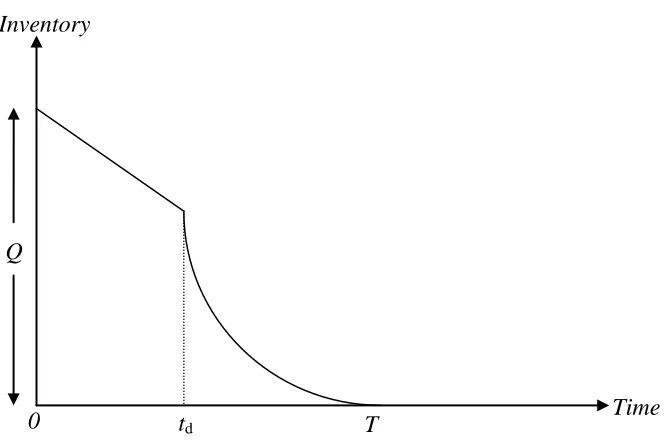
The inventory system evolves as follows: Q units of items arrive at the inventory system at the beginning of each cycle. The inventory level is declining only due to demand rate over time interval [0, td]. The inventory level is reducing to zero owing to demand and

deterioration during the time interval [td, T].The process is repeated as mentioned above. The

pattern of inventory level is depicted in Figure 1.

 

1

, 0 _d

dI t

D t t

dt     (1)

 

 

2

2 , d

dI t

I t D t t T

dt      (2)

[image:4.612.150.482.201.422.2]

with terminal condition I₁

 

0 Q and I T₂

 

0.

Figure 1: The graphical representation for the inventory system

The solution to (1)–(2) is,

 

1 , 0 d

I t  Q Dt  t t (3)

 



 



2

1 ,

T t

d d e

I t t t T





 _

   (4)

Since I t₁

 

I₂

 

t at tt_d, it follows from (4) and (5) that,

 



T t 1



d d e Q dt





 _

 

which yields the order quantityQ, as

 



T t 1



d d

Q t e





 

 _   _ (5)

Inventory

Q

Time

td T

1. The ordering cost is K

2. The holding cost is

 

 

2



 





 







1 2 2

0 1 1 2 d d d d

T t T t

t T _d d d

t

e t e T t

t

h I t dt I t dt hD

  _      _{   }   _ _{    }        





3. The deterioration cost is

 







2





 







1 d

T t

d

d d d d

e T t

c I t D T t c D

 _    _{  }          

Assembling above cost components, the total costper unit of time (denoted by TC (T)) is given by

  

ordering cost holding cost deterioration cost



TC T   

 











 







2 2 1 1 2 d d

T t T t

d d

d

d

e t e T t

D t K

h h c

T T   _        _   _{  }   _{   }  _    _      _{   }   (6)

4.2 Fuzzy inventory model

In this study, we have characterized the demand rateD, as a triangular fuzzy number to tackle the reality in more effective way.Thus, the objective function defined in (10) can be constructed under fuzzy framework as follows:

 



1

 

, 2

 

, 3

 



FTC T  FTC T FTC T FTC T (7)

where,

  

1



2



 









 







1 2

1 1

2

d d

T t T t

d d

d

d

e t e T t

D t K

FTC T h h c

T T   _         _   _{  }   _{    }  _    _      _{   }   (8)

 

2



 









 







2 2

1 1

2

d d

T t T t

d d

d

d

e t e T t

D t K

FTC T h h c

T T   _        _   _{  }   _{   }  _    _      _{   }   (9)

  

2



2



 









 







3 2

1 1

2

d d

T t T t

d d

d

d

e t e T t

D t K

FTC T h h c

In order to obtain equivalent deterministic form of (7), we employ Graded Mean Integration Representation method proposed by Chen and Hsieh (1999) which is based on the integral value of graded mean α-level of generalized fuzzy number.If A



a₁, ,a a₂



be a TFN, then the modified graded mean integration representation ofTFNAis

 



1



4



2



6

a a a

P A      (11)

Through Eqs. (8) – (10) and using formula (11) we have

 





1

 

4 2

 

3

 

6

FTC T FTC T FTC T

P FTC T    (12)

Thus, the problem is reduced to

 





Minimize Subject to _d

P FTC T

T t

(13)

Our objective is to determine the optimalcycle time which minimizes the total cost per unit time in fuzzy sense. For this, we set first order derivative of P FTC T



 



with respect to T to be zero,

i.e.dP FTC T



 



dT 0. (14)

The non-linear nature of objective function in (12) indicates that it is notpossible to obtain closed form solution. However, using Maple 14, the local solutionis obtained in the next section.

4. Numerical example

Example 1: An inventory system with the following data is considered.

D7000 units/year, h = $ 2/unit/year, K = $ 150 / order, c_d  $ 20 / unit, t_d  15/365 year,

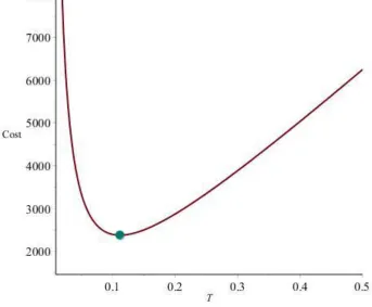
  0.08,  ₁ 50, ₂ 150. Solving Eq. (14) by Maple 14 gives T*  0.1121 year, Q* 

[image:7.612.145.488.45.328.2]

Figure 2: Convexity of P FTC T



 



with respect to T

Example 2:In this example we shall assess the impact of the extent of impreciseness in demand

rate over the decision variable. For this, let us first consider the crisp inventory model with same set of input data as in Example 1 except  ₁ 0, ₂ 0.

The crisp model gives the optimal result asT*  0.1122 year, *

Q  786.81 units and

 

*

TC T $2376.75.

[image:8.612.61.547.56.422.2]

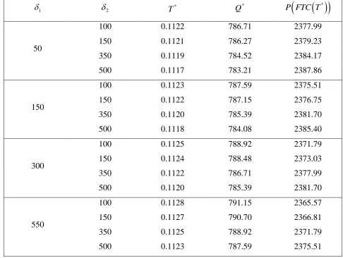
Table 1: Optimal solution for different values of ₁ and ₂ 1

 2 T*

*

Q P FTC T



 

*



50

100 0.1122 786.71 2377.99

150 0.1121 786.27 2379.23

350 0.1119 784.52 2384.17

500 0.1117 783.21 2387.86

150

100 0.1123 787.59 2375.51

150 0.1122 787.15 2376.75

350 0.1120 785.39 2381.70

500 0.1118 784.08 2385.40

300

100 0.1125 788.92 2371.79

150 0.1124 788.48 2373.03

350 0.1122 786.71 2377.99

500 0.1120 785.39 2381.70

550

100 0.1128 791.15 2365.57

150 0.1127 790.70 2366.81

350 0.1125 788.92 2371.79

500 0.1123 787.59 2375.51

From the Table 1 it can be observed that for fixed value of₁, the optimal length of replenishment cycle (T*) andthe optimal order quantity (Q*) decrease whereas the optimal cost in fuzzy sense increases with an increase in the value of 2. On the other hand, for fixed value of₂, the optimal length of replenishment cycle (T*) and the optimal order quantity (Q*) increase whereas the optimal cost in fuzzy sense decreases with an increase in the value of ₁. It may also interesting to note that when demand rate

 

D be symmetrical TFN then the optimal results are equivalent to crisp case (see the results when ₁ = ₂ = 150).

5. Conclusion

Furthermore, we illustrated the behavior of our model with respect to key parameters in numerical examples.

The work presented herein could have several possible extensions. For example, this model can be extended to accommodate shortages, variable deterioration rate, stochastic demand, and so forth. One could also incorporate the different preservation investment in the model formulation.

References

[1] Chang, C.T., Teng, J.T., Goyal, S.K., 2010. Optimal replenishment policies for non-instantaneous deterioratingitems with stock-dependent demand. International Journal of Production Economics, 123, 62–68.

[2] Chang, H. J., Lin, W. F., 2010. A partial backlogging inventory model for non-instantaneous deteriorating items with stock-dependent consumption rate under inflation. Yugoslav Journal of Operations Research, 20, 35–54.

[3] Chen, S. H., Hsieh, C. H., 1999. Graded mean integration representation of generalized fuzzy number. Journal of Chinese Fuzzy Systems, 5, 1–7.

[4] Ouyang, L. Y., Wu,K. S., Yang,C. T., 2006. A study on an inventory model for non-instantaneous deteriorating items with permissible delay in payments.Computers and Industrial Engineering, 51, 637–651.

[5] Ouyang, L. Y., Wu,K. S., Yang,C. T., 2008. Retailer’s ordering policy for non-instantaneous deteriorating items with quantity discount, stock dependent demand and stochastic backorder rate. Journal of Chinese Institute of Industrial Engineers, 25, 62– 72.

[6] Shah, N. H., Soni, H. N., Patel, K. A., 2013. Optimizing inventory and marketing policy for non-instantaneous deteriorating items with generalized type deterioration and holding cost rates. Omega, 41, 421 – 430.

[7] Soni, H. N., Patel, K. A., 2013. Joint pricing and replenishment policies for non-instantaneous deteriorating items with imprecise deterioration free time and credibility constraint. Computers & Industrial Engineering, 66, 944–951.

[9] Wu,K. S., Ouyang,L. Y.,Yang, C. T., 2006. An Optimal Replenishment Policy for Non-instantaneous Deteriorating Items with Stock-dependent Demand and Partial Backlogging.International Journal of Production Economics, 101, 369 – 384.

[10] Wu,K. S., Ouyang,L. Y.,Yang, C. T., 2009. Coordinating replenishment and pricing policies for non-instantaneous deteriorating items with price-sensitive demand.International Journal of Systems Science, 40, 1273–1281.