Munich Personal RePEc Archive
Patents as Collateral
Chatelain, Jean-Bernard and Ralf, Kirsten and Bruno,
Amable
Université Paris 1 Panthéon Sorbonne, Paris School of Economics,
ESCE Ecole Supérieure du Commerce Extérieur
2010
Patents as Collateral
Bruno Amable
y, Jean-Bernard Chatelain
z, Kirsten Ralf
xJournal of Economic Dynamics & Control (2010) 34 1092-1104
Post Print
Abstract
This paper studies how the assignment of patents as collateral deter-mines the savings of …rms and magni…es the e¤ect of innovative rents on investment in research and development (R&D). We analyse the behaviour of innovative …rms that face random and lumpy investment opportunities in R&D. High growth rates of innovations, possibly higher than the real rate of interest, may be achieved despite …nancial constraints. There is an optimal level of publicly funded policy by the patent and trademark o¢ce that minimizes the legal uncertainty surrounding patents as collateral and maximizes the growth rate of innovations.
Keywords: Collateral, Patents, Research and Development, Credit ra-tioning, Growth, Innovation.
JEL Codes: D92, G24, G32, O16, O41, O34.
“It is the uncertainty created by this legal and regulatory structure [in the United States] which leads to the very market imperfections
The authors thank three anonymous referees of this journal for helpful comments and con-structive suggestions. All remaining errors are our own.
yCES (Centre d’Economie de la Sorbonne), Université Paris 1 Panthéon Sorbonne, Paris
School of Economics, 106-112 boulevard de l’Hôpital, 75647 Paris Cedex 13. Email: [email protected]
zCES (Centre d’Economie de la Sorbonne), Université Paris 1 Panthéon Sorbonne, Paris
School of Economics, 106-112 boulevard de l’Hôpital, 75647 Paris Cedex 13. Email: [email protected]
xESCE (Ecole Supérieure du Commerce Extérieur), 10 rue Sextius Michel, 75015 Paris.
Email: [email protected]
and ine¢ciencies currently minimizing the ability to leverage the value of intellectual property assets and consequently stunting the economic growth of inventors and entrepreneurs,” Murphy (2002) report to the United States Patent and Trademark O¢ce (USPTO).
1. Introduction
The practice of using a valuable patent portfolio as collateral for a debt assignment
is slowly becoming more and more important in the United States and elsewhere.1
It follows a start-up stage …nanced by venture capital where the …rm obtained at least one valuable patent. After an initial public o¤ering, many innovators still lack the capital necessary to develop new research and must turn to outside sources for funding. For these innovative …rms, there is now considerable empirical evidence that variables related to …nancing constraints such as debt/assets ratio and/or cash ‡ow availability are correlated with R&D investment (see Hall’s (2002) sur-vey). Due to the limited availability of physical capital as collateral, innovators face an external …nance constraint. With asymmetric information on the state of the R&D project, additionally, problems of adverse selection and moral hazard
occur. Blundell, Gri¢th and Van Reenen (1999) explain: “A more traditional
in-terpretation of the innovation-market power correlation is that failures in …nancial markets force …rms to rely on their own supra-normal pro…ts to …nance the search for innovation. The availability of internal sources of funding (‘deep pockets’) are useful for all forms of investment, but may be particularly important for R&D”. In the knowledge economy, wealth creation is increasingly based on innovation that, in turn, can give rise to important intellectual property rights. For many companies, these intellectual property rights represent their most valuable assets. Patent-backed loans increase the availability of external funds and the return on equity for the shareholders.
In the United States, the potential e¤ect of patent-backed loans on the growth of innovation is estimated to be important for the following reasons. First, the stock of potential untapped intangible collateral is by now huge. Corrado, Hulten
1Since the end of the 1990s, several IPR intermediaries services (Ocean Tomo and Patent
and Sichel (2006)2 estimate investment in intangible assets to be $1.2 trillion
per year for the period 2000-2003 (a level of investment that roughly equals the gross investment in corporate tangible assets), including $230 billion in innovative property of scienti…c R&D, besides innovative property of non-scienti…c R&D and computer software. Depending on its depreciation rate, the stock of intangible assets may be …ve to ten times this level of investment. Second, post initial public o¤ering (IPO) shareholders of innovative …rms have a strong monetary incentive to use patent-backed debt instead of new share issues: no dilution of capital and a leverage multiplier e¤ect on their return on equity. Third, the patent backed loan industry is fostered by intellectual property rights (IPR) lawyers, IPR valuation, technology and …nancial intermediaries and IPR insurance …rms, who lobby for the required legal and regulatory changes to be supported by the USPTO. Fourth, the share of measured innovations (patents, R&D spending) by older …rms owning at least one valuable patent (that could be used as collateral) is much larger than
the one of start-ups …nanced by venture capital in the United States.3 The pool
of innovative …rms with new projects, likely to use patent-backed loans, is broad. Kiyotaki and Moore’s (1997) and Kiyotaki’s (1998) seminal papers deal with the magnifying e¤ects of collateral availability constraints in order to explain business cycles movements. Their framework paved the way to new studies of monetary policy and housing prices (Iacoviello (2005)) or asset prices, the credit channel, liquidity in closed or open economies (e.g. Faia and Monacelli (2007), Gertler, Gilchrist and Natalucci (2007), Kato (2006), Kunieda and Shibata (2005), Moretto and Tamborini (2007), Bougheas, Mizen and Yalcin (2006), Cordoba and Ripoll (2004), Amable, Chatelain and Ralf (2004), Chatelain (2001)). Kiyotaki and Moore’s (1997) framework also tackles the issue of lumpy and irreversible investment, leading to recent extensions by Caggese (2007) and Sveen and Weinke (2007). Lumpiness is also an observed characteristic of R&D investment in lab equipment (Geroski, Van Reenen and Walters (1997), Aghion et al. (2007)). But collateral issues remained con…ned to business cycles theory.
This paper introduces patents as collateral in the context of expanding variety growth models dealing with intellectual property rights (Rivera Batiz and Romer
2In their table 2.
3Kamiyama, S., J. Sheehan and C. Martinez (2006) mention that high value patents are
(1991), Amable et Chatelain (1995), Kwan and Lai (2003), Boucekkine and de la Croix (2003), Donoghue and Zweimüller (2004), Barro and Sala-I-Martin (2004), Gancia and Zilibotti (2005), Strulik (2007), Furukawa (2007)). These papers already discussed various arguments for and against intellectual property rights granting monopoly rights to patent holders. The novel point here is to consider the prospective consequences of a large development of the use of patents as collateral on economic growth, as this practice is likely to spread in the next decades.
The paper has three goals: Firstly, it provides the condition for a signi…cant leverage e¤ect of the collateral assignment of patents on the growth of innovation. It shows in particular that the dependence of innovations on past innovations
increases with innovative rentsrelatively more than in standard expanding variety
growth models based on R&D (Romer and Rivera Batiz (1990), Barro and Sala-I-Martin (2004)). Secondly, it models the …nancial constraints on individual …rms savings, the aggregate debt-equity ratio, and economic growth. Finally, we show that the rate of return of innovation is higher than the credit interest rate in a growing economy and that the growth of patents is a decreasing function of the interest rate. This is not the case in the standard R&D endogenous growth models. The model di¤ers from the Kiyotaki and Moore’s (1997) credit cycle model in various ways: the size of the aggregate capital stock is no longer …xed, but may grow over time, and expected monopoly rents on existing patents are used as collateral, so that they increase the value of collateral, the available amount of loans and economic growth. The model is the …rst one dealing with the assignment of patents as collateral in the economic literature.
the growth of innovations. Moreover, the model speci…es how such a leverage may lead to high speed growth of the knowledge economy. A credit constraint based on the value of already existing patents rules out Ponzi …nance, so that a high speed growth rate of innovations may exceed the interest rate on patent backed loans in equilibrium.
The paper is organized as follows. The microeconomic behaviour of agents is described in section 2. Section 3 provides the conditions for steady state aggregate growth. Section 4 concludes the paper with a discussion of the results and related research.
2. The model
We consider a lab-equipment model of expanding variety (Rivera-Batiz and Romer (1991), Barro and Sala-I-Martin (2004)), which is directly related to R&D invest-ment equations estimated in applied work (Blundell et al. (1999)). As in other “increasing product variety” models (Romer (1990), Grossman and Helpmann (1991)), the economy has three sectors of production: a …nal goods sector, whose price is taken as numeraire, an intermediate goods sector, whose output is used in the production of the …nal good and an R&D sector in which blueprints allowing the creation of new intermediate goods are discovered.
2.1. Households
A constant population of wage-earning households is distributed on [0; L]. A
household maximizes utility over an in…nite time horizon:
Ut = P+1
=0 u(ct+ ) with u(ct) = (c1t 1)=(1 ) for > 0 and 6= 1 or
with u(ct) = ln (ct) for = 1. ct 0 is consumption in t, 0 is the rate of
time preference, = 1=(1 + )is the discount rate and is the relative ‡uctuation
aversion. Households supply inelastically one unit of labour used in the …nal goods
industry and are paid a real wage ratewt. They have no disutility of labour. They
lend to entrepreneurs and earn a rate of return rt on their wealth bht. The law of
motion of their wealth isbht = (1+rt 1)bth 1+wt ct. The initial wealthbh0 is given
and identical for all households. Taking into account the optimum consumption
plan of the households, consumption growth gc is given by
1 +gc;t+1 =ct+1=ct =Ct+1=Ct= ( Rt)
1
where Ct =ctL denotes aggregate household consumption and Rt = 1 +rt. The
growth rate of household consumption increases with the return on savings and decreases with the rate of time preference and with the relative ‡uctuation aversion
.
2.2. Production of the …nal good
A large number of producers of the …nal good, indexed by j, operate in perfect
competition. Producerj produces the quantityYjt according to a constant return
to scale production function:
Yjt =L1jt Z Nt
0
Xjt(i) di with 0< <1: (2)
A producer uses labour and intermediates as inputs that are fully used up within
the period. Xjt(i) is the amount of intermediate good i used by producer j on
a set fXjt(i); i 2 [0; Nt]g. Nt represents the most recently invented intermediate
good, so that the interval [0; Nt] is the variety of intermediate goods available
in the economy. The representative producer of …nal goods maximizes pro…t while buying intermediate goods. This leads to the following demand function for intermediate inputs:
Xjt(i) =
pit
1=(1 )
Ljt for i2[0; Nt]: (3)
2.3. Production of intermediate goods
The …rm producing an intermediate non-durable good, indexed by i, acts as a
monopolist selling to …nal good producers at a price which adds a mark-up to
marginal costs. A rent it has to be paid to the innovator for using his blueprint
at each datet. Production of intermediate goods takes place at constant marginal
cost, normalized to 1. Taking into account the demand for intermediate inputs
(see equation (3)), the producer of an intermediate good maximizes
max
pit
it= (pit 1) X
j
Xjt(i): (4)
The solution for the monopoly price is
pit =p=
1
Hence, the pricepit is constant over time and the same for all intermediate goods
i. The aggregate quantity of each intermediary good produced and the monopoly
pro…t are also constant over time, whereas the aggregate level of …nal outputYt is
proportional to the number of intermediate goodsNt. Output net of intermediate
goods is then:
Yt XNt =
1
+ 1 Nt: (6)
2.4. R&D sector: technology and …nance
Every period, a continuum of risk neutral entrepreneurs distributed over the
inter-val [0;1]is engaged in the R&D activity. On date0, each entrepreneur k receives
an initial dividend d0;k that he spends on consumption and has an initial
endow-ment of n0;k of valuable blueprints.4 The aggregate number of patents on date 0
is denoted N0 and aggregate dividends D0.
Utility is given as the expected present value V0 of dividends dt 0. Future
dividends are discounted using the market interest rate rt. E0 is the expectation
operator at date 0:
Choose nt; bt; it; dt that maxV0 =E0
"
d0+ =+1
X
=1
d
T=
T=1(1 +rT) #
: (7)
The entrepreneur maximizes his utility. He chooses the state variables which
are the stock of patentsntand the stock of debtbt, (with given initial endowments
b0;k and n0;k) by changing the control variables: new patentsit and dividends dt.
His utility is subject to constraints. First, there are two equality constraints: the law of motion of patents derived from the innovation process, the law of motion of debt (or net worth) derived from the ‡ow of funds constraint. Second, there are two inequality constraints: the saving ceiling (or minimal consumption, or positive dividend) and the debt ceiling.
Innovation on date t depends on two factors: The entrepreneur has to have new ideas and he has to provide his …rm speci…c labour. The …rst factor accounts for the fact that the entrepreneur may …nd a number of positive net present value
ideas leading to new valuable patents (1it>0 = 1; where it is the number of new
blueprints obtained in a period) only with probability (0< 1). With
prob-ability 1 , he will have no ideas (1it>0 = 0). This factor is motivated by the
4The following model of aggregate growth of innovations holds for all types of initial
observation that R&D lab-equipment investment is lumpy (Geroski, Van Reenen,
Walters (1997)). The value of the random variable1it>0 is known by the
entrepre-neur at the beginning of the period t, but is not observable for the creditor. The
second factor accounts for the fact that the entrepreneur may supply inelastically
one unit of R&D speci…c labour (ht = 1) in her own …rm, without disutility of
labour, or withdraw her labour (ht= 0) leading to zero investment in R&D. This
assumption captures the informational asymmetry between lenders and innova-tors describing a problem of moral hazard. It is too costly for lenders to enforce loan repayment with an ex post assessment discriminating zero investment related
to “not working” versus zero investment related to “having no ideas” (1it>0 = 0).
The fact that the labour input of the entrepreneur is R&D speci…c and cannot be carried out by a hired worker enables us to avoid labour sectoral allocation problems as in Romer (1990). The stock of blueprints of the entrepreneur evolves then according to the following equation:
nt= 1it>0 ht it+ (1 )nt 1 (8)
where 0 is a hazard rate related to the opposition and litigation due to an
identical, close or overlapping prior innovation, so that the related intermediate
goods disappear.5
The ‡ow of funds constraint states that dividends are equal to the pro…t at
date t earned from previously discovered blueprints plus new debt net of interest
repayment minus cost of investment in R&D:
dt=
q qnt 1 rt 1bt 1+bt bt 1 1it>0 ht q (nt nt 1): (9)
whereq is the unit cost per patent granted: the cost function of R&D investment
is linear when the entrepreneur does invest:
1it>0 ht q (nt (1 )nt 1):
5A patent examiner must …nd evidence of prior art which can be elusive. Hence, litigation
Minimal consumption constraint: Entrepreneurs consume a minimum amount
dm 0 which is written as a proportion (1
0
) of …rms net worth (equity).
0
1 is then the entrepreneurs savings rate. If 0
= 1, the entrepreneur may
not consume anything and we get the usual assumption that dividends are greater than or equal to zero. Dividends have to be larger than the minimum consumption required by the entrepreneur:
dt dm = (1
0
) ( qnt 1 Rt 1bt 1) 0; (10)
where = 1+q (assuming a positive net return of innovation: 0 q <1),
Rt 1 = 1 +rt 1.
Financing: patents as collateral. A large number of risk neutral and perfectly competitive …nancial intermediaries pool households savings in order to diversify the risks related to the use of patents as collateral. An entrepreneur has always the
ability to threaten its creditors to withdraw his labour input (ht = 0), repudiate
his debt contract, consume at the end of the period the stock of debt bt and its
rate of return rtbt and …nd other creditors for next periods (Kiyotaki and Moore
(1997)). This incentive to cheat exists as soon as the end of period value of the stock of debt is larger than the expected value of the ‡ow of new patents denoted vt+1(it): (1 +rt)bt > vt+1(it): In case of default, a lender receives a
random proportion, , 0 1 of the value of the collateral. The value of
the debt, therefore, should not exceed the discounted market value of the sum of existing patents for each entrepreneur. When patents are used as collateral, the entrepreneur has no longer an incentive to withdraw labour, because he will lose
his stream of future incomes, so that: ht= 1.
The loan to patent portfolio value =(1 + rt) depends on the Patent O¢ce
public spending. This key assumption takes into account that lenders are not perfectly protected against the borrower’s ability to transfer, abandon or license the patent collateral to a third party or to competing creditors at no legal costs (Schavey, 2003; Murphy, 2002). Lenders pool patent backed loans so that they
take into account the expected proportion 0 1 of the next period value
of the current patent portfolio assigned as collateral Vt+1(nt) when deciding the
occurs because lenders protect themselves by limiting the amount of the loan:6
(1 +rt)bt Vt+1(nt) with (11)
Vt+1(nt) = nt " 1 + +1 X =1 (1 ) T=
T=1(1 +rT) #
:
The patent portfolio nt provides its …rst return nt on date t+ 1. When the
collateral constraint is not binding, we assume that there is free entry into the
business of being an inventor so that any entrepreneur can pay the R&D costqnt
to secure the net present value Vt+1
1+rt. Free entry leads to a zero pro…t condition:
qnt=
Vt+1(nt)
1 +rt
: (12)
The equilibrium interest rate with free entry is rF =
q . When borrowing
constraints hinder entry, then one has:
qnt=
Vt+1(nt)
1 +rF <
Vt+1(nt)
1 +rt
: (13)
The limitations on borrowing at the interest rtprevent that an in…nite amount of
resources would be channelled into R&D at time t. The credit constraint may be
written as a “leverage” or debt/patent ratioxt bounded by an endogenous ceiling
xc (the last equality holds for a steady state interest rate: r
t=r):
xt=
bt
qnt
xc = 1 +rt
Vt+1(nt)
qnt
=
q(r+ ): (14)
Innovators’ behaviour: To sum up, entrepreneurs maximize their utility, with
control variablesit and dt, and state variables nt and bt, n0 and b0 given:
V0 =E0
"
d0+
t=+1
X
t=1
dt T=t
T=1(1 +rT) #
6This assumption corresponds to current practice. Financial and intellectual property rights
subject to equality constraints
nt = 1it>0 it+ (1 )nt 1;
dt =
q qnt 1 rt 1bt 1+bt bt 1 1it>0q(nt nt 1);
and to inequality constraints
0 qntxc bt;
0 dt (1
0
) ( qnt 1 Rt 1bt 1):
Substituting consumption from the ‡ow of funds equation (9) into the saving ceiling constraint (10) and using the debt ceiling constraint (14), one …nds an upper limit on the growth of innovations determined by the ceiling of internal savings and by the debt ceiling:
(1 xc)qnt+ 1it>0 1 q(nt nt 1)
0
( qnt 1 Rt 1bt 1): (15)
When an innovator has an opportunity to invest (1it>0 = 1), and when x
c 1
(that is when q > rt), the above constraint does not set a ceiling on the stock
of patents nt, but a negative ‡oor which is not constraining patents.
Condition 1: q < rt< q .
When the interest rate satis…es condition 1, patents are limited by:
qnt
0
( qnt 1 Rt 1bt 1)
1 xc : (16)
The growth rate of patents is also limited due to the collateral constraint on the number of patents (11) and the ‡ow of funds equation (9).
The solution of the optimization program of the entrepreneur is summarized in the following proposition:
Proposition 1. Optimal R&D Investment, Saving and Borrowing at the Entrepreneur Level.
In each period, innovating …rms can be in one of three regimes: (i) Perfect capital market regime: rF
(ii) Currently binding credit constraint regime: With probability the inno-vator has an opportunity to invest at date t and faces binding debt and patents ceilings:
bt=xcqnt=
Vt+1(nt)
1 +rt
(17)
qnt=
0
( qnt 1 Rt 1bt 1)
1 xc : (18)
(iii) Anticipated credit constraint regime: With probability1 , the innovator has no opportunity to invest and saves as much as possible in order to decrease debt. Then:
bt=qnt 1 0
( qnt 1 Rt 1bt 1)< bt 1: (19)
In regime (i), the debt ceiling never binds, debt policy does not a¤ect R&D investment.
Financially constrained regimes (ii) and (iii) are obtained under the condition 1 that the credit interest rate is below the marginal return of R&D investment
rt < q . The entrepreneur consumes his minimal level of consumption (dt =
dm). In regime (iii), the size of the patent portfolio declines due to depreciation:
nt = (1 )nt 1: (20)
If an entrepreneur has a long history of no opportunity to invest in R&D, he may eventually become a net creditor. When an entrepreneur which has built “deep pockets” over a history of no pro…table ideas faces an opportunity to invest,
he invests as much as allowed by the …nancial constraint due to his linear cost
function and because the marginal return on R&D exceeds the credit interest rate. A proof of proposition 1 can be found in appendix 1.
Additional remarks: The assumption of discounting …rms’ dividends by the interest rate is common to most of neo-classical and endogenous economic growth models. This assumption leads to a straightforward comparison of the …nancially constrained growth regime with the perfect capital market growth regime of the lab-equipment model presented in Barro and Sala-I-Martin (2004). In business cycles models with collateral constraints, the usual assumption is to assume that …nancially constrained entrepreneurs discount the logarithm of their dividends by
a subjective discount factor denoted distinct from households discount factor
3. High Growth of Innovations with Collateral Constraints
In this section we will analyse the steady state solution of the above model. In order to do this, we calculate …rst the steady state aggregate debt/patent ratio (debt and patents grow at the same rate in a steady state). Secondly, we …nd the equilibrium interest rate such that households’ consumption grows also at the steady state growth rate. In what follows, we assume additionally that R&D
investment is not lumpy ( = 1).7 Then the innovator can only be in the perfect
capital market regime or in the current binding credit regime. In the latter, debt is a linear function of the stock of patents (equation 17) at the microeconomic level. Hence, the dynamics of aggregate debt is identical to the dynamics of aggregate patents. The patents equations are linear in patent and debt, so that aggregation across entrepreneurs does not require to keep track of the distribution of the individual entrepreneurs’ patents and debt. Aggregate patents and debt
are denoted by capital letters Nt and Bt. Since the population of entrepreneurs
is unity, the aggregate number of patents is limited by the sum of patent ceiling inequalities (16):
qNt
0
( qNt 1 Rt 1Bt 1)
1 xc : (21)
The above inequality is an equality when condition 1 is ful…lled (…nancially con-strained regime).
Equilibrium on the …nal goods market occurs if total consumption, i.e. ag-gregate consumption of households plus agag-gregate consumption of entrepreneurs, equals output in the …nal goods sector net of intermediate goods minus the amount of resources devoted to R&D activity:
Ct+Dt =Yt NtX q(Nt+1 Nt):
Aggregate consumption of the entrepreneur is equal to aggregate dividends and
can be expressed as a proportion of the number of patents.8 Since output net of
7The case of lumpy R&D investment ( <1) is treated elsewhere by the authors. 8Expressing the debt level as a fraction of the debt ceiling B
t= 0x qNt, with0 < 0 1
and 0= 1 in the …nancially constraint regime we get:
Dt = 1 00 ( qNt 1 Rt 1Bt 1)
Dt = 1 00 ( Rt 1 0x )
intermediate goods is also proportional to the number of patents (see equation
(6)) and q(Nt+1 Nt) = qgNt, where g is the growth rate of patents, aggregate
household consumption is proportional to the number of patents. In a steady state growth path all these aggregates therefore grow at the same constant rate.
Households’ aggregate consumption growth rate follows fromCt+1 = ( (1 +rt))
1
Ct.
The endogenous interest rate rt ensures the equality of demand and supply of
funds. When the interest rate is equal to the marginal return of innovation
rt = q , the free entry steady state growth factor of patents is equal to
Nt+1=Nt = ( )1= . The growth rate is positive as long as the interest rate is
higher than the households’ rate of time preference. This growth level can be reached only if it is below the maximal rate of growth of patents allowed by the
…-nancial constraint whenrt = q is equal to
0
. Else, the …nancially constrained growth rate prevails.
Condition 2 for …nancially constrained growth:
0
<
1 1 1
(22)
Entrepreneurs’ saving rate of equity 0
is su¢ciently low (or equivalently the en-trepreneurs’ rate of time preference is su¢ciently high).9
Proposition 2: Steady State Growth Regimes
When condition 2 is not ful…lled, the free entry equilibrium prevails. The interest rate is equal to the return of R&D investment and there exists a unique steady state growth factor ( )1= . When condition 2 is ful…lled, there exists a unique steady state interest rate r that is lower than the marginal return on R&D investment and there exists a unique …nancially constrained steady state growth factor G =GC(r ) =GN(r ).
Proof Under condition 2, an equilibrium interest rate r determines a
con-strained steady state growth rateg . The growth rate of consumption equals the
9If the householdsï¿1
2relative ‡uctuation aversion, is equal to one, condition 2 boils down to
entrepreneurs’ saving rate of net worth lower than households’ saving rate of net worth: 0< . Although several recent papers dealing with collateral constraints assumed 0< , in national accounts, …rms’ savings rate is often higher than households’ savings rate (a key assumption of Kaldorian models of growth and distribution (Bertola, Foellmi and Zweimüller (2006)). Here, the entrepreneursï¿1
2 savings rate of net worth can be higher than households savings rate when
maximal growth rate of patents:
H(r) = 0
+ ( R) 1
1 xc(r) 1 ( (1 +r))
1=
= 0:
AsH is a continuous and strictly decreasing function of the interest rate over the
interval
max ;
q ;q ; as limr! q H(r) = +1>0
and as H q < 0 (condition 2), there exists an unique equilibrium interest
rate, corresponding to an unique strictly positive patent growth rate, according to the intermediate value theorem.
Remark: When dividends are always zero ( 0
= 1), condition 2
<( )
1
is the equivalent of a no-Ponzi-game hypothesis, ruling out
chain-letter debt …nance. Chain-chain-letter debt …nance can be seen as taking ever larger amounts of debt in order to pay o¤ the debt of the previous period plus interest. Then, the steady state growth rate with perfect capital market is below the free
entry rate of interest rF =
q . This particular no-Ponzi-game condition sets a
minimal level for the relative ‡uctuation aversion (strictly below unity) in order to slow down the free entry steady state growth (Barro and Sala-I-Martin (2004)), so that chain-letter debt …nance is not feasible:
1 + ln ( )
ln ( ): (23)
However, this condition on a minimal level of the relative ‡uctuation aversion is no longer necessary when there is a binding collateral constraint, which also rules out chain-letter debt …nance, hence proposition 3:
Proposition 3: Financially constrained growth rate higher than the real interest rate is feasible.
held view, …nancial constraints are compatible with high level of the growth of in-novation, because collateral leverages growth. However, the growth rate cannot exceed 1 + 1
q, else consumption is zero.
As debt is always fully backed by a correct evaluation of the value of available collateral at all future periods, lenders avoid repayment problems related to Ponzi …nance (see also Araujo et al. (2002)). It is not necessary to add an alternative no-Ponzi …nance condition such that, in an equilibrium, the growth rate has to be lower than the interest rate, nor to assume overlapping and growing generations.
In the real world, Ponzi …nance arises when lenders lendmore than the expected
value of collateral and/or when they systematically over-estimate the long-term
value of collateral when there is an asset price bubble. There remains a ceiling (higher than the interest rate) to the growth rate, because R&D investment should
[image:17.612.208.407.356.510.2]not totally crowd out households consumption, which has to remain positive.10
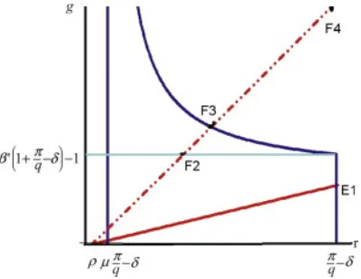
Figure 1 below presents a graphical representation of the steady state with the growth rate on the vertical axis and the interest rate on the horizontal axis.
Fig. 1. Equilibrium growth rates as a function of real interest rates.
We distinguish two cases of relative risk aversion of households: the rising line
starting from the value of time preference = 1% with the higher slope rising
line corresponds to = 0:5, the one with the lower slope corresponds to = 2.
They show all possible growth rates for a given interest rate. The parameters for
innovative …rms are set as follows: q = 5%, = 1, 0
= 0:98. A vertical line
10If there are some …rms that are not able to invest, <1, we get transitional dynamics for
on the left side of the …gure represent the asymptote of the …nancially constrained
patent growth rate: r = q = 1:25% for = 0:25. On the right of this
asymptote, the patent growth curve for = 0:25 is …rst represented by a curve
decreasing with interest rate as long as:
q = 1:25% < r < q = 5%
with a growth rate higher than 0
1 = 2:9%. For growth rate below 0
1 =
2:9%, the patent growth rate curve is represented by a vertical line: r= q =
5%, because of the free entry condition in capital markets. We can consider four
steady state growth regimes (Table 1).
1:25% < r 5% g
E1 2 0 1 5% = q 2%< 0
1
F2 0:5 !0 2:5% 2:9% = 0
1
F3 0:5 25% 2:9% 3:8%
F4 0:5 !1 5% = q 8;1%
Table 1. Steady state growth rates and interest rates.
In equilibrium E1 there is a high relative ‡uctuation aversion( = 2)and
con-dition 2 is not ful…lled: the free entry steady state growth prevails. For equilibria with a low relative ‡uctuation aversion of households that is households do not satisfy the bounded utility condition (23), the growth rate increases with , from
the “no debt” regime with = 0 (F2), to the = 25%(F3). The theoretical limit
case of perfect collateral ( = 100%) is not possible in practice with patents as
collateral, where the free entry growth rate level can be reached even when the growth rate exceeds the real interest rate (F4).
Proposition 4: Policy e¤ects of Murphy’s (2002) legal reforms on patents growth. Public expenditures may shift the economy from equilibrium F2 to equilibrium F3, with a sharp increase of the growth of innovations.
Murphy (2002) proposes to raise public expenditures in the USPTO and in the IPR public legal system in order to reduce the uncertainty surrounding the use of patents as collateral for lenders and the costs of litigation on transfers of IPR, for example, by funding a public registry of patents used as collateral. The proportion
of the value of patents transferred to lenders (G=N) = 0(G=N)a (with 0 >0
and with elasticity a > 0) increases with G=N, which measures public funding
per patent devoted to grease the wheels of the transfers of property rights in IPR
when patents are used as collateral (with 0
with a proportion (0 <1) the rent of each patent currently registered at the USPTO. An alternative public funding leading to similar results consists of a corporate income tax with a deduction of interest payments. This taxation also
decreases the collateral market value of each patent by a factor(1 ). The tax
policy maximizing the growth of patents amounts to maximize the after tax rate of return on equity of innovative …rms (written in a way to simplify the derivative with respect to the tax rate):
max
2
4r+ (1 )q (r+ ) 1 0( )a(1 )q
r+
3
5:
The tax rate increases the proportion of the value of patents transferred to lenders, but decreases the value of patents, and decreases the ‡ow of pro…ts. The trade-o¤ between the …rst two e¤ects leads to the tax rate maximizing the debt/patent
ratioxc (at the denominator of the growth rate) which is
= a 1 +a:
Because the tax rate also decreases the ‡ow of pro…ts and hence the growth
rate, the growth maximizing tax rate is below the loan/patent ratio maximizing
tax rate: 0 < < . This solution is an interior solution as long as the after
tax pro…ts remain positive, that is when: 1 q(r+ )= , else this upper
bound prevails as a corner solution. This corner solution disappears when one taxes corporate income after interest payments. After tax pro…ts (net of interest
payments) are then always positive. The growth maximizing tax rate is given
by the implicit equation:
q (1 x
c( )) = (1 )
q (r+ )
@xc( )
@ :
The reform is such that the economy shifts from 0(very few patent backed
loans, with a suboptimal level of public expenditures equal to zero: G=N = = 0)
to a widespread practice of patent backed loans, with an aggregate loan to patent
ratio ( )=(1 +r), expected to be close to 25% in practice (Edwards (2002)).
This e¤ect of this policy is evaluated using the growth di¤erential following a
shift from equilibrium F2 to equilibrium F3: G( ( )) 0
. Under condition
the policy e¤ect on the growth rate of innovation may be huge. The growth rate
increases from2:9% to 3:9% and the interest rate increases from2:5% to2:9%.
Additional information can be gained when we compute the marginal e¤ect of policy reforms on growth:
@GN
@ = ( (1 +r ))
1
1
@gN @ @gC
@r
@gN @r
>0 (24)
with
@gN
@ =
0
q r
@x
@xcq(r + )
(1 x )2 >0:
A large e¤ect of a marginal change of the loan to patent ratio is obtained for
a large gap between the equilibrium credit interest rate and the marginal return on innovation. Graphically, the closer the equilibrium interest rate is to the value of the real interest rate determining the vertical asymptote of the patent growth curve, the larger the marginal e¤ect on growth of reducing the legal uncertainty surrounding patents as collateral.
4. Conclusion
This paper describes an endogenous growth model with lenders limiting credit up to the collateralizable value of existing patents and with a composition between innovative …rms facing a probability to …nd a positive net present value R&D investment opportunity or not each period.
First, at the entrepreneur level, …nancial constraints and lumpiness lead to a speci…c entrepreneurs savings behaviour where they build “deep pockets” by antic-ipating future …nancial constraints. When a lumpy R&D investment opportunity occurs, the dependence of the persistence of R&D investment on the mark-up rewarding innovations is ampli…ed by the debt/patent collateral constraint.
Secondly, the aggregation of entrepreneurs behaviour determines a steady state endogenous aggregate leverage (or debt/patent ratio) below the leverage ceiling.
Extensions suggest that collateral assignment of patents may be detrimental to open source, because it adds incentives to value patents portfolios. Leverage driven growth is a necessary characteristic of high speed growth of innovation.
Appendix A. Proof of proposition 1
The Lagrangian of the entrepreneur program is:
(nt; bt) 2 ArgmaxE0 +1
X
t=1
Lt T=t
T=1(1 +rT)
with Lt = 1 + dt dt+ bt(qxcnt bt)
+ dt( (1 0
) ( qnt 1 Rt 1bt 1))
where bt is the Lagrange multiplier related to the debt ceiling constraint, dt is
the Lagrange multiplier related to the minimal consumption constraint, and with
consumptiondt given by the ‡ow of funds constraint:
dt = ( qnt 1 Rt 1bt 1) +bt qnt 1it>0 1 q(nt nt 1):
The Euler equation on debt bt is @L@btt = 0, for any date t:
0 = 1 + dt bt+Et
(1 +rt) 1 + dt+1 + dt+1(1 0
) (1 +rt)
1 +rt+1
!
)
d
t = bt 1 + (1 +rt)Et
1 + 0 d
t+1
1 +rt+1
!
:
The …rst order condition with respect to the stock of patents is @Lt
@nt = 0, that is:
0 = 1 + dt ( q) +qxc bt
+Et
1 1 +rt+1
1 + dt+1 h q+ 1it+1>0 1 q
i
+Et
1 1 +rt+1
d
t+1( (1 0
One divides byq and substitutes dt using the …rst order condition for debt:
0 = bt (1 +rt)Et
1 + 0 d t+1
1 +rt+1
!
+xc bt
+ 1 +
q Et
1 + 0 d t+1
1 +rt+1
!
+Et
1 + dt+1 1 +rt+1
!
1it+1>0 1 :
Hence:
q rt= (1 x
c) bt
Et
1+ 0 d t+1
1+rt+1
+Et 0
@ 1 + d
t+1 (1 1it+1>0)
1 + 0
Et dt+1
1
A:
The su¢cient conditions as stated in Chow (1997), p.29, are also ful…lled, since the functions are concave and either the Lagrange parameter is equal to zero and the inequality condition not binding or the Lagrange parameter is di¤erent from zero and the inequality condition is binding, see Chatelain (2000).
Appendix B. Logarithmic Utility for Entrepreneurs
This appendix considers the case where entrepreneurs maximize a (concave)
logarithmic utility, with a discount factor = 1=(1 + 0
) which may di¤er from
households discount factor11:
+1
X
=0
ln(dt+ ) (25)
subject to the ‡ow of funds constraint, the collateral constraint, and the positive
consumption constraintdt 0. The Euler equation on debt bt is @L@btt = 0, for any
date t:
0 = 1
dt
+ dt bt+
Et (1 +rt) dt1+1 + dt+1
1 + 0 )
d
t = bt
1
dt
+ (1 +rt) Et
1
dt+1
+ dt+1 : (26)
11This discount factor plays the same role as the maximal saving rate of equity when
The …rst order condition with respect to the stock of patents is @Lt
@nt = 0, that is:
0 = 1
dt
+ dt ( q) +qxc bt
+q ( )Et
1
dt+1
+ dt+1
+q Et
1
dt+1
+ dt+1 1it+1>0 1 :
One divides byq and substitutes dt using the …rst order condition for debt:
q rt = (1 x
c)
b t
Et
1
dt+1+
d t+1
1+rt+1
+Et 0
@ 1 + d
t+1 (1 1it+1>0)
Et dt1+1 + dt+1
1
A:
a) Case where bt = dt+1 = 0 and 1it+1>0 = 1, the Euler equation for patents
and on debt leads to:
dt+1
dt
= = (1 +rt):
Hence rt 1 = q =rt, so that the ‡ow of funds constraint can be written as a
function of the entrepreneur’s equity:
qnt bt =Rt 1(qnt 1 bt 1) dt: (27)
Using the Euler equation for debt, one has:
Rt 1 =Rt 1
dt
qnt 1 bt 1
:
Hence:
dt= (1 ) (qnt 1 bt 1)
with the entrepreneur’s net worth on datet de…ned byat= (qnt 1 bt 1). The
savings of an entrepreneur are a fraction of her …rm net worth at. A balanced
growth where the growth rate of households consumption is equal to the growth
factor of entrepreneurs consumption is obtained when households utility is
also logarithmic with an identical discount factor = , or in the particular case
b) Case where bt >0and dt+1 >0and1it+1>0 = 1,rt 1 < q : entrepreneurs invest by borrowing up to the credit limit because the rate of return on their R&D investment exceeds the real interest rate. The debt ceiling constraint can be written as:
at+1 = qnt (1 +rt)bt= 1
q(r+ ) 1 +rt
qnt:
When the debt ceiling constraint binds, the ‡ow of funds constraint can be written as:
qnt=
qnt 1 Rt 1bt 1 dt
1 xc :
Hence, the entrepreneur net worth is:
at+1 =
1 xc1+rt
1 xc (at dt):
Maximizing the log utility of dividends determined by the entrepreneur net worth
constraint implies that the saving of an entrepreneur is a fraction of her …rm
net worth at. When all …rms do invest and are …nancially constrained on date t
and date t 1, and the growth factor of patents is equal to the growth rate of
households consumption in the steady state, which may lead to an equilibrium
interest rate below its free entry levelrt 1 < q :
+
q rt 1 xc
1 xc = [ Rt 1]
1
under condition2:
<[ ]1 :
When = 1 (households utility is also logarithmic), then condition2 means that
the discount factor of entrepreneurs is lower than the discount factor of households
< (entrepreneurs rate of time preference discount the future more heavily than
households).
Appendix C. Steady state debt/patent ratio
The law of motion of the debt/patent ratio xt as a function of its previous
value: xt=M(xt 1) is computed using the aggregate patent growth factor:
Nt
Nt 1
=G =
1 xc
0
and the aggregate debt (or equity) law of motion, which can be written as:
Nt
Nt 1
=GF =
0
( Rt 1xt 1)
1 xt
= 0
+ Rt 1
xt 1
xt
1 1 xt
1 :
The steady state leads to the implicit relationN(xt; xt 1) =GF G = 0:
N(xt; xt 1) = 0
( Rt 1xt 1)
1 xt 1 xc
0
( Rt 1xt 1) (1 ) (1 ) = 0:
which can be written as this explicit equation:
xt = M(xt 1; rt 1) = 1
0
( Rt 1xt 1)
1 xc
0
( Rt 1xt 1) + (1 ) (1 )
= 1 1 x
c 0
@1 1
1 + 1 xc
0( R
t 1xt 1)
(1 )(1 )
1
A: (29)
A su¢cient condition for @M
@xt 1 <1:
@M @xt 1
=
0
Rt 1(1 ) (1 )
1 xc
0
( Rt 1xt 1) + (1 ) (1 ) 2 <1
rt 1 <
1
0
(1 ) (1 ) 1<
G2 0
(1 ) (1 ) 1) (30)
@M @xt 1
< 1:
The steady state debt/patent ratioxis given by the following quadratic equation:
N(x; x)
0 =
Rt 1x
1 x 1 xc ( Rt 1x)
(1 ) (1 )
0 = 0:
The function N(x; x) is continuous on the interval[0; xc] and strictly increasing:
@N(x; x)
@x =
0 Rt 1
(1 x)2 +1 xcRt 1 >0:
According to the intermediate value theorem, a unique solution exist for a positive
steady state debt/patent ratio 0< x xc <1 under the conditions N(0;0)<0
and N(xc; xc)>0. First,N(xc; xc)>0is always ful…lled as long as <1 :
N(xc; xc) = (1 ) 0
+ ( Rt 1)
xc
Second,N(0;0)<0 leads to condition 2, such that should not be to low:
N(0;0) = (1 xc) [ 0
(1 ) (1 )] 0
<0
) xc = q
r+ > x
c
min = (1 )
0
(1 )
0
(1 ) (1 ) :
Condition 2 for the steady state debt/patent ratio to be strictly positive implies
that the interest rate should be below the ceiling rmax:
r < rmax=
xc
min q
:
The explicit solutionx is found by solving the quadratic equation N(x; x) = 0.
References
[1] Aghion, P., Askenazy, P., Berman, N., Cette, G., Eymard, L., 2007. Credit constraints and the cyclicality of R&D investment: evidence from France. mimeo. Harvard University.
[2] Amable, B., Chatelain, J.-B., 1995. Systèmes …nanciers et croissance: les e¤ets du "court-termisme". Revue Economique, 46(3), 827-836
[3] Amable, B., Chatelain, J.-B., Ralf, K., 2004. Credit rationing, pro…t accu-mulation and economic growth. Economics Letters 85, 301-307.
[4] Araujo, A., Pascoa, M.R., Torres-Martinez, P., 2002. Collateral avoids Ponzi schemes in incomplete markets. Econometrica 70, 1613-1637.
[5] Barro, R., Sala-I-Martin, X., 2004. Economic Growth, second ed. MIT Press, Cambridge (Mass).
[6] Bertola, G., Foellmi, R., Zweimüller, J., 2006. Income Distribution in Macro-economic Models. Princeton University Press;, Princeton.
[7] Blundell, R., Gri¢th, R., Van Reenen, J., 1999. Market share, market value and innovation in a panel of British manufacturing …rms. Review of Economic Studies 66, 529-554.
[9] Bougheas, S., Mizen, P., Yalcin, C., 2006. Access to external …nance: Theory and evidence on the impact of monetary policy and …rm-speci…c characteris-tics. Journal of Banking and Finance 1, 199-227.
[10] Caggese, A., 2007. Financing constraints, irreversibility, and investment dy-namics. Journal of Monetary Economics 54, 2102-2130.
[11] Chatelain, J.-B., 2000. Explicit Lagrange multiplier for …rms facing a debt ceiling constraint. Economics Letters 67, 153-158.
[12] Chatelain, J.-B., 2001. Mark-up and capital structure of the …rm facing un-certainty. Economics Letters 74, 99-105.
[13] Chow, G.C., 1997. Dynamic Economics. Oxford University Press.
[14] Cordoba, J.C., Ripoll, M., 2004. Credit Cycles Redux. International Eco-nomic Review 45, 1011-1046.
[15] Corrado, C. A., Hulten, C. R., Sichel, D. E., 2006, Intangible capital and economic growth, NBER Working Paper No. 11948, NBER, Cambridge, MA.
[16] Donoghue, T., Zweimüller, J., 2004. Patents in a Model of Endogenous Growth. Journal of Economic Growth 9, 81-123.
[17] Edwards D., 2002. Patent backed securitization: blueprint for a new asset
class <http://www.securitization.net/pdf/gerling_new_0302.pdf>.
[18] Faia, E., Monacelli, T., 2007. Optimal interest rate rules, asset prices, and credit frictions. Journal of Economic Dynamics and Control 31, 3228-3254.
[19] Furukawa, Y., 2007. The protection of intellectual property rights and en-dogenous growth: Is stronger always better? Journal of Economic Dynamics and Control 31, 3644-3670.
[20] Gancia, G., Zilibotti, F., 2005. Endogenous Growth with Product Variety, in: Aghion, P. and Durlauf, S. (eds.). The Handbook of Economic Growth. North-Holland.
[22] Gertler, M., Gilchrist, S., Natalucci, F.M., 2007. External Constraints on Monetary Policy and the Financial Accelerator. Journal of Money, Credit and Banking 39, 295-330.
[23] Grossman, G.M., Helpman, E., 1991. Innovation and Growth in the Global Economy. The MIT Press, Cambridge, MA.
[24] Hall, B.H., 2002. The Financing of Research and Development. Oxford Re-view of Economic Policy 18, 35-51.
[25] Iacoviello, M., 2005. House Prices, Borrowing Constraints, and Monetary Policy in the Business Cycle. American Economic Review 95, 739-764.
[26] Kamiyama, S., Sheehan, J., Martinez, C., 2006, Valuation and exploitation of intellectual property, OECD Science, Technology and Industry Working Papers, 2006/5, OECD Publishing.
[27] Kato, R., 2006. Liquidity, in…nite horizons and macroeconomic ‡uctuations. European Economic Review 50, 1105-1130.
[28] Keuschnigg, C., 2004. Venture Capital Backed Growth. Journal of Economic Growth 9, 239-261.
[29] Kiyotaki, N., Moore, J., 1997. Credit Cycles. Journal of Political Economy 105, 211-248.
[30] Kiyotaki, N., 1998. Credit and Business Cycles, Japanese Economic Review 49, 18-35.
[31] Kunieda, T., Shibata, A., 2005. Credit constraints and the current account: A test for the Japanese economy. Journal of International Money and Finance 24, 1261-1277.
[32] Kwan, F.Y.K, Lai, E.L.C., 2003. Intellectual Property Rights Protection and Endogenous Economic Growth. Journal of Economic Dynamics and Control 27, 853-873.
[34] Murphy, W.J., 2002. A proposal for a centralized and integrated registry for security interests in intellectual property. IDEA The Journal of Law and Technology. Franklin Pierce Law Centre, Concord, USA 41, 297-601 (41 IDEA 297).
[35] Rivera-Batiz, L., Romer, P., 1991. Economic Integration and Endogenous Growth. Quarterly Journal of Economics 106, 531-55.
[36] Romer, P., 1990. Endogenous Technological Change. Journal of Political Economy 98, S71- S102.
[37] Serrano, C.J., 2008. The dynamics of the transfer and renewal of patents. NBER working paper.
[38] Schavey, R.D., 2003. Security Interest in Patents and
Trade-marks. Mayer, Brown, Rowe and Maw LLP Publication,
http://www.securitization.net/pdf/Ru¤
[39] Strulik, H., 2007. Too much of a good thing? The quantitative economics of R&D Driven Growth revisited. Scandinavian Journal of Economics 109, 369-386.