Munich Personal RePEc Archive
Levy subordinator model: A two
parameter model of default dependency
Balakrishna, B. S.
28 October 2010
Online at
https://mpra.ub.uni-muenchen.de/32882/
L´evy Subordinator Model :
A Two Parameter Model of Default Dependency
B. S. BALAKRISHNA
∗October 28, 2010
Revised: August 18, 2011
“There is no “right” model. The best you can do is pick a model that mimics the most important behavior of the underlyer in your market. Then add perturbations if necessary.”
– Emanuel Derman in “Modeling the Volatility Smile”.
Abstract
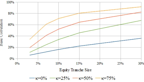
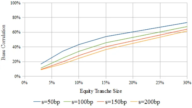
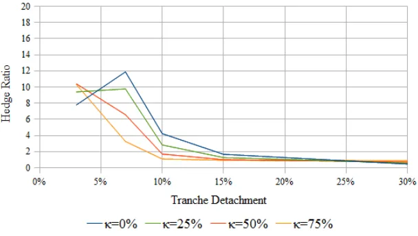
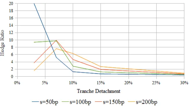
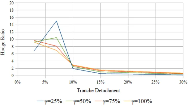
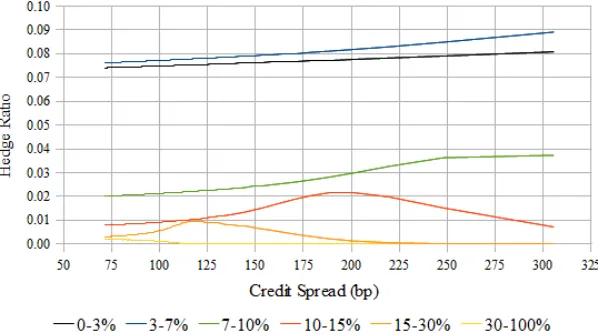
The May 2005 crisis and the recent credit crisis have indicated to us that any realistic model of default dependency needs to account for at least two risk factors, firm-specific and catastrophic. Unfortunately, the popular Gaussian copula model has no identifiable support to either of these. In this article, a two parameter model of default dependency based on the L´evy subordinator is presented accounting for these two risk factors. Subordinators are L´evy processes with non-decreasing sample paths. They help ensure that the loss process is non-decreasing leading to a promising class of dynamic models. The simplest subordinator is the L´evy subordinator, a maximally skewed stable process with index of stability 1/2. Interestingly, this simplest subordi-nator turns out to be the appropriate choice as the basic process in modeling default dependency. Its attractive feature is that it admits a closed form expression for its dis-tribution function. This helps in automatic calibration to individual hazard rate curves and efficient pricing with Fast Fourier Transform techniques. It is structured similar to the one-factor Gaussian copula model and can easily be implemented within the framework of the existing infrastructure. As it turns out, the Gaussian copula model can itself be recast into this framework highlighting its limitations. The model can also be investigated numerically with a Monte Carlo simulation algorithm. It admits a tractable framework of random recovery. It is investigated numerically and the implied base correlations are presented over a wide range of its parameters. The investigation also demonstrates its ability to generate reasonable hedge ratios.
Modeling dependent events and their correlations has remained a challenging issue. An understanding of its implications is needed for pricing derivative instruments referencing a collection of credit names, and it is a subject of interest outside the realm of credit derivatives as well. Many models have been developed for pricing the correlation products, but the market standard has remained the Gaussian copula model in spite of all the criticisms it received for its alleged role in the recent credit crisis. As has been emphasized by many, it has been well-known that the Gaussian copula model has serious limitations and is inadequate as a model of default dependency.
Major attraction of the Gaussian copula model is its simplicity and tractability. It can easily be calibrated to individual hazard rate curves. It can be formulated in closed form providing a semi-analytical framework for pricing. It admits efficient pricing with recursive methods or Fast Fourier Transform techniques. As we will see in this article, there exists another simple and tractable model similar in architecture that also enjoys these properties. Unlike the Gaussian copula model, it is a dynamical two-parameter model capable of offering a reasonable explanation of the correlation smile. The two parameters provide the two measures necessary to assess dependency risk, a measure of correlation and that of the likelihood of a catastrophe. The model is based on the L´evy subordinator, anα= 1/2 stable process maximally skewed to the right, whose distribution function is expressible in closed form and is known as the L´evy distribution. Though it is inevitable that, with a model of such few parameters, there is bound to exist a residual smile, the ability to capture the smile characteristics will be helpful in sensitivity analysis and stress testing.
Issues with the Gaussian copula model have been addressed before. Brigo, Pallavicini and Torresetti [2010] provide a discussion of its limitations and an account of the developments in this field. They also note that, since the start of the credit crisis, the probability mass associated to a catastrophic or armageddon event, i.e. the default of the entire pool of credit references, has increased dramatically. The need for such a catastrophic scenario while pricing the super-senior tranche was noted earlier by many authors, see for instance Balakrishna [2009]. However, in many of the models, such a scenario needs to be enforced, somewhat artificially. An attractive feature of the subordinator models discussed here is that such a scenario arises naturally as a consequence of a drift term that is well-known to be a natural component of the dynamics of subordinators.
During the earlier May 2005 crisis, a so-called correlation dislocation is said to have taken place. As has been pointed out by many, this is attributable to increased firm-specific risk. The May 2005 crisis and the recent credit crisis have thus indicated to us that any realistic model of default dependency needs to account for at least two risk factors, firm-specific and catastrophic. Unfortunately, the Gaussian copula model has no identifiable support to either of these. The two risk factors necessitate introduction of at least two parameters into any realistic model of default dependency as in the models discussed in this article.
rates. An important virtue of the Gaussian copula model is that it has no such additional intensity-like variables. As we will see in this article, the subordinator models discussed here share this virtue as they too have no additional intensity-like variables.
Models of the volatility smile have taught us that an explanation of the smile alone is not a guarantee for obtaining satisfactory hedge ratios. Local volatility models, though capable of providing a perfect fit to the smile, are criticized for giving rise to hedge corrections inconsistent with typical market behavior. Models respecting some concept of stationarity have been pursued to obtain better hedge ratios. Within the context of the correlation smile, subordinator models discussed here attempt to achieve a similar goal. Numerical investigation of the L´evy subordinator model demonstrates its ability to generate reasonable hedge ratios under a wide range of its parameters.
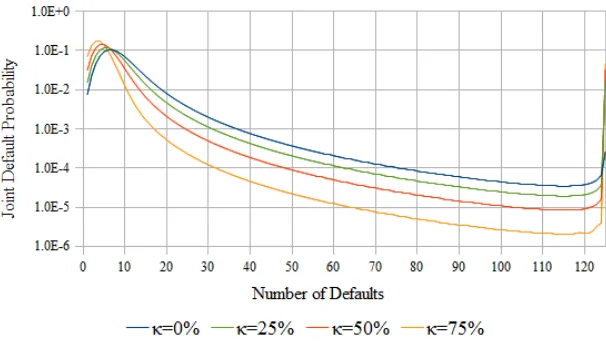
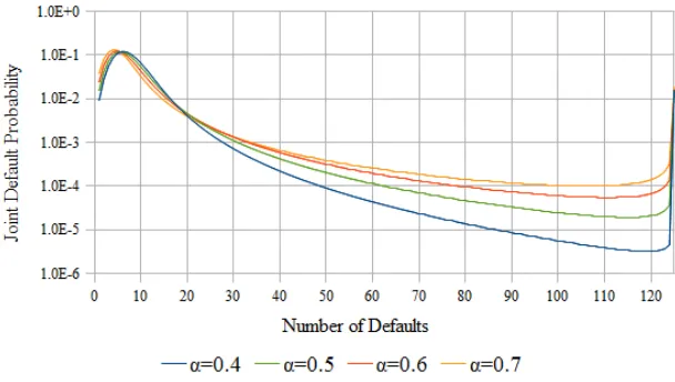
In Balakrishna [2007] and some of the literature in the field, it is found that the modeled loss distribution displays one or more bumps along its tail. Even if such a distribution is able to reproduce the market prices providing an explanation of the correlation smile, it is not immediately obvious whether the bumps are a realistic feature of the distribution or an artifact of the model. Models capable of reproducing the market prices without such bumps, even if less accurate, can potentially give rise to better behaved prices and sensitivities. As it turns out, the L´evy subordinator model presented here exhibits no such bumps along the tail of its default probability distribution.
1
A Brief on Subordinators
L´evy processes, and hence subordinators, is a well researched branch of mathematics. For the sake of completeness, the following gives a brief review of subordinators.
A stochastic process is an indexed family of random variables. A continuous-time stochas-tic process is such a process indexed over continuous time. A L´evy process is a continuous-time stochastic process starting as zero that has independent and stationary increments, and is stochastically continuous. Independence is a statement that increments over disjoint time-intervals are independent random variables. Stationarity is a statement that incre-ment over any time-interval is distributed with its time-dependence only on the length of the time-interval. Stochastic continuity means that jumps are random and rare, that the probability of a jump occurring at a given time is zero. A realization or a sample path of a stochastic process is a sampling of each of the random variables in the family. Subordinators are real-valued L´evy processes with non-decreasing sample paths.
Given a subordinator X(t), its Laplace transform, or equivalently its Laplace exponent η(u), is given by
e−tη(u) = Ee−uX(t) , u≥0, (1)
where E{}denotes expectation value. The specific time-dependence assumed for the Laplace transform above is a consequence of the properties of the subordinator as a L´evy process. It follows that the Laplace exponent of a sum of two independent subordinators is the sum of their Laplace exponents. An important result for L´evy Processes is the L´evy-Khintchine formula. In the case of subordinators, it gives for the Laplace exponent
η(u) =bu+
Z ∞
0
λ(dy) 1−e−uy. (2)
Here b ≥ 0 is called the drift coefficient that contributes a non-negative drift bt to X(t) so that X(t) ≥ bt for all t. λ(dy) is called the L´evy measure that is required to satisfy
R∞
0 λ(dy)min(y,1)< ∞. It is also true that any function of the above form is the Laplace
exponent of a subordinator.
An important subclass of subordinators are stable subordinators. Their Laplace exponent isη(u) = auα+bu for some constanta and index of stabilityα ∈(0,1), obtainable from the
L´evy measure aα[Γ(1−α)]−1y−1−αdy. Stable subordinators are also a subclass of stable
processes having index of stability α ∈ (0,1) and maximally skewed to the right, that is, their skew parameter set to one. It follows that stable subordinators (more generally stable processes) feature an additive property, that is if X(t) andY(t) are two independent stable subordinators with index of stability α (and parameters bX, aX and bY, aY), then Z(t) =
pX(t) +qY(t) is also a stable subordinator with index of stabilityα (havingbZ =pbX+qbY
and aZ =pαaX +qαaY).
Inversion of the Laplace transform gives us the probability density function of the random variable X(t) at time t, or equivalently its cumulative distribution function gt(x) given by
gt(x) = E1X(t)≤x , (3)
where 1{···} is the indicator function. No closed form expression is available for gt(x) in
L´evy subordinator1. In the case of the L´evy subordinator that has η(u) = a√u+bu, the
distribution is known as the L´evy distribution and is given by
gt(x) = 2N
−at/p2(x−bt),
∂xgt(x) =
1
2√πat(x−bt)
−3/2e−14(at)2/(x−bt), (4)
where N() is the cumulative standard normal distribution function. This includes a non-negative drift component bt discussed above so that gt(x) and ∂xgt(x) can be taken to be
zero for x < bt.
L´evy distribution (4) is also the first passage time distribution of a Brownian motion over time variable x≥bt with the barrier set at at/√2. The first passage time distribution of a Brownian motion with drift rate c√2, that is of a Gaussian process, is also available in closed form and is known as the inverse Gaussian distribution. The associated subordinator is the inverse Gaussian subordinator that has η(u) =a √u+c2−c+bu and
gt(x) = N(−at/z +cz) +e2actN(−at/z−cz),
∂xgt(x) =
2 √
2πate
actz−3e−1
2((at)2z−2+c2z2), z =p2(x−bt). (5)
Though not a stable subordinator, inverse Gaussian subordinator is useful as the natural extension of the L´evy subordinator. Its L´evy measure is that of the L´evy subordinator damped exponentially with e−c2y
. Other stable subordinators are also generalized in this way with an exponential damping called tempering of the L´evy measure.
Stable subordinators feature a scaling property such that (at)−1/α(X(t)−bt) is
indepen-dent of tin distribution, that isgt(x) is a function of the combination (at)−1/α(x−bt). This
scaling property is evident in the behavior of the tail of their distributions. The long tail of the distribution of a stable subordinatorX(t) obeys a power-law decay with
gt(x+bt)→1−at[Γ(1−α)]−1x−α, for large x. (6)
At the very short end, the log-distribution exhibits a power-law behavior with
−lngt(x+bt)→(1−α) α(at)1/α
α/(1−α)
x−α/(1−α), for small x. (7)
A consequence of the power-law decay for large x is that stable subordinators have both infinite mean and infinite variance.
The scaling property enables one to express the distribution function gt(x) for any stable
subordinator in terms of that of a standardized random variableZ. Random values ofZ can be generated using Kanter’s method (special case of the Chambers-Mallows-Stuck method for a stable distribution) from two independent random numbers: an exponentially distributed
1
W with unit mean and a uniformly distributedθ ∈(0, π) (see for instance Zolotarev [1986]). For the stable subordinator standardized to yield η(u) =uα, this can be obtained as
Z = sin(αθ) sin(θ)
sin ((1−α)θ) Wsin(θ)
(1−α)/α
. (8)
The distribution function fα(z) of Z thus computed depends on just α and hence can be
used at any time t to obtain gt(x) =fα(z) given z = (at)−1/α(x−bt), x > bt.
The most basic subordinator is the Poisson process havingη(u) = λ(1−e−u). It has
unit-size jumps occurring at intensityλ. The form of the Laplace exponent in (2) indicates that a subordinator should be constructible from Poisson processes with varying jump sizes. L´evy-Itˆo decomposition theorem applied to subordinators provides us with such a construction that reads, in the differential form,
dX(t) =bdt+
Z ∞
y=0
ydN(λ(dy), t). (9)
Here N(λ(dy), t) is a Poisson process of intensity λ(dy) associated with the interval (y, y+ dy) and dN(λ(dy), t) is its increment over the time interval (t, t+dt). Poisson increments associated with disjoint t and disjoint y intervals are independent random variables. If N(λ(dy), t) jumps up by one at time t, dN(λ(dy), t) causes X(t) to jump up byy at time t. Over an infinitesimal time interval (t, t+dt), we have
E{exp [−uydN(λ(dy), t)]}= exp−dtλ(dy) 1−e−uy. (10)
This follows simply on noting that dN(λ(dy), t) takes values zero and one with probabilities 1− dtλ(dy) and dtλ(dy) respectively, irrespective of the value of N(λ(dy), t). It is now straightforward to obtain the Laplace exponent (2) summing up contributions arising from disjoint t and disjointy intervals.
2
One Factor Formulation
It is instructive to proceed formulating the model starting with an infinitely large homoge-neous collection of credit names. This offers an intuitive insight into its structure that has a basis in probability theory due to a theorem attributed to de Finetti. The model then evolves as a natural extension of this formulation.
Given an infinite homogeneous collection of credit names, consider a configuration of its defaulted and undefaulted states at some future time t. Let us say our interest is not in the actual assignment of states among the names, but only on the fraction of names in the defaulted states. The collection being infinite, this fraction ν can take any value from zero to one. The configuration is thus characterized by just one common risk factor that is identifiable with the fraction ν.
defaulted is ν2. More generally, the probability of finding a set of j names defaulted and k
names undefaulted is νj(1−ν)k. In other words, the states can be treated as independent
variables. If the configuration under consideration itself has a probability density function ∂νFt(ν), Ft(ν) being the cumulative default distribution function, the probability of finding
j names defaulted and k names undefaulted can hence be written as
P[j,k](t) =
Z 1
0
dν∂νFt(ν)νj(1−ν)k. (11)
This is a one-factor formulation since, given a value of just one variableν, defaults get treated as independent random variables. This intuitive result has a basis in probability theory due to a theorem attributed to de Finetti. It is sometimes helpful to express Ft(ν) in terms of a
random variable V(t) taking values in [0,1] as
Ft(ν) = E
1V(t)≤ν . (12)
Random variables V(t) for all t > 0 with V(0) = 0 can be viewed together as defining a stochastic process that we may denote for simplicity as V(t) itself.
Some general characteristics of Ft(ν) can be inferred to start with. It is of course a
non-decreasing function of ν. As the May 2005 crisis has indicated, there can be firm-specific contributions to defaults and hence, in a realistic model, one expects a minimum value νmin(t) for ν below which Ft(ν) = 0. This is because firm-specific contributions are
mutually independent and hence, in an infinitely large homogeneous collection, one expects at least a fraction of names equal to the firm-specific default probability to have defaulted. Further, it has been usual to consider Ft(ν)→ 1 as ν → 1. But, as the recent credit crisis
has indicated, there can be a non-zero probability for all the names in the collection to have defaulted by time t so that Ft(ν) should be allowed to tend to some Fmax(t) <1 as ν →1.
Forν in-between, Ft(ν) is expected to be a decreasing function of t. Note that V(t) can not
be decreasing as a function oft since we do not allow for recovery of defaulted names. Given two times t1 and t2, t1 < t2, we have
Ft1(ν)−Ft2(ν) = E
1V(t1)≤ν−1V(t2)≤ν = E
1V(t1)≤ν,V(t2)>ν −E
1V(t1)>ν,V(t2)≤ν . (13)
For a non-decreasing stochastic process V(t), the last expectation above is zero. Assuming that there are nonzero contributions to the first term, as is usually the case, we thus have Ft1(ν)> Ft2(ν) forν in-between.
Formulation (11) has all the complexities of the model bundled into one common function Ft(ν). We may proceed with it by modelingV(t), but there is an interesting and more flexible
alternate formulation that emphasizes individual behavior. Let us rewrite (11) as
P[j,k](t) =
Z 1
0
dF[pt(F)]j[1−pt(F)]k, (14)
where pt(F) is the inverse of Ft(ν) defined by pt(Ft(ν)) = ν, ν ≥ νmin(t). Because Ft(ν) is
Generic characteristics of Ft(ν) discussed above imply similar ones for pt(F).
Equiva-lently, they can be inferred fromF viewed as an indicator of economic conditions, with higher F corresponding to less favorable circumstances. Conditional individual survival probability qt(F) = 1− pt(F) is a non-increasing function of F for all t > 0. With F = 1
corre-sponding to the worst case scenario, that of total collapse with all the names defaulting, we have qt(1) = 0. A non-zero probability of such a scenario implies that qt(F) = 0 for some
F ≥Fmax(t). At the F = 0 end, the common variables are ineffective in causing defaults so
that qt(0) is firm-specific. As noted earlier, Ft(ν) for ν in-between is a decreasing function
of t. Consequently, for F in-between, qt(F) is decreasing as a function of t, starting at one
and ending up at zero as t runs from zero to infinity.
The characteristics ofqt(F) suggest that 1−qt(F)/qt(0) can be viewed as the cumulative
distribution function of a random variable Φi(t) taking values in [0,1]. In other words,
qt(F) = qt(0)E
1Φi(t)≥F . (15)
Random variables Φi(t) for all t > 0 can be viewed together as defining a stochastic
pro-cess, denoted for simplicity as Φi(t) itself. It is a non-increasing process with Φi(0) = 1
and Φi(∞) = 0. There is one such independent stochastic process for each name in the
collection, hence the name-subscript. In the homogeneous collection under discussion here, they are identically distributed. For the unconditional individual default probability P(t), or equivalently its survival counterpart Q(t) = 1−P(t), we then have
Q(t) =
Z 1
0
dF qt(F) = qt(0)E Z 1
0
dF1Φi(t)≥F
=qt(0)E{Φi(t)}. (16)
Satisfying this ensures that the model gets calibrated to individual hazard rate curves. Models based on formulation (11) are referred to here as type-I models. Note that there is only one stochastic processV(t) in its one-factor formulation modeling the common factor. Many reduced form models belong to this class. Intensity based models that have a systemic component to their stochastic default intensities are type-I models. BecauseV(t) is directly related to the loss process (for uniform recovery rates), many loss process models can also be viewed as type-I models.
In contrast, formulation (14) appears new. Here the collection, though homogeneous, has one independent stochastic process Φi(t) for each of its names. A model of these Φi(t)s is
referred to here as a type-II model. These models are in some sense like structural models. It turns out that the popular copula models can be reformulated as belonging to this class. The reformulation highlights their unnaturalness modeling Φi(t)s as static objects. Interestingly,
as we will discover, there also exist new models, perhaps more promising, that model Φi(t)s
as genuinely dynamic stochastic processes.
3
Finite Heterogeneous Collection
to an infinite one. The two formulations result in different models depending on the choices made forV(t) or Φi(t)s. The following introduces further extensions of the two homogeneous
versions to heterogeneous collections.
Consider type-I formulation (11) to start with. It is convenient to work with Λ(t) = −ln[1−V(t)], a non-decreasing process taking values in [0,∞] with Λ(0) = 0 and Λ(∞) =∞. The joint survival probability QΩ(t) for a list of names in Ω can then be expressed as
QΩ(t) = E
e−Pi∈ΩΛi(t) . (17)
A name-subscript i has been attached to Λ(t) to make it applicable to a heterogeneous collection. Since we had only on process V(t) to start with, expectation E{} is taken with respect to a common process X(t) in a one factor formulation. All Λi(t)s are considered
to be driven by X(t), for instance as Λi(t) = aiX(t) +bit for some parameters ais and bis.
Expression (17) indicates that defaults are independent given a realization of X(t). For the unconditional individual survival probability Qi(t), we now have
Qi(t) = Ee−Λi(t) . (18)
Satisfying this ensures that the model gets calibrated to individual hazard rate curves. Type-II formulation (14) can be similarly generalized to a finite heterogeneous collection. Here too, it is convenient to work with Λi(t) = −ln Φi(t) for each name, a non-decreasing
stochastic process taking values in [0,∞] with Λi(0) = 0 and Λi(∞) =∞. The conditional
default and survival probabilities pt(F) and qt(F) = 1−pt(F) are now denoted with
name-subscripts as pi(F, t) and qi(F, t) respectively. Integration variable F may now be viewed
simply as a uniformly distributed common factor. In terms of Λi(t),qi(F, t) reads
qi(F, t) = qi(0, t)E1Λi(t)≤−lnF . (19)
For the unconditional individual survival probability Qi(t) we then have
Qi(t) =qi(0, t)Ee−Λi(t) . (20)
Satisfying this ensures that the model gets calibrated to individual hazard rate curves. The joint survival probability QΩ(t) for a list of names in Ω can be expressed as
QΩ(t) =
Z 1
0
dF Y
i∈Ω
qi(F, t) = "
Y
i∈Ω
qi(0, t) #
Ee−Maxi∈ΩΛi(t) , (21)
where Maxi∈Ω picks up the largest Λi(t) in Ω. This follows from the fact that Λi(t)s are
independent stochastic processes. It is interesting to note that this defines the model with no reference to the common factor that has been integrated away. Dependency is built into the combination Maxi∈ΩΛi(t).
the joint survival probability of a list of names in Ω is e−Maxi∈ΩΛi(t) (here and below, it is
assumed that they have survived their firm-specific risk factors). Consider further just two names in Ω say 1 and 2, and a realization with Λ1(t) ≤ Λ2(t). The probability of both
the names having survived during (0, t) is e−Λ2(t). Since the survival probability of name 2
irrespective of the state of name 1 is also e−Λ2(t), this implies that it is not possible to have
name 1 defaulted and name 2 survived. If name 1 has defaulted, then name 2 should have defaulted as well. More generally, without loss of generality, consider a realization with the ordering Λ1(t)≤ Λ2(t)≤ · · ·. In this ordering, if name i is known to have defaulted during
(0, t), all names labeledj > i should have defaulted as well. That is, if a common crisis has resulted in name i defaulting, then all names known to be more vulnerable to the crisis in a realization should have defaulted as well. Stated this way, maximum dependency appears to be more realistic than the conditional independence formulation of expression (17). Besides, some contagion effects appear to be already in place.
The F−formulation can be viewed as realizing the Λi(t) processes further to obtain
an assignment of defaulted and undefaulted states. This follows after re-introducing the F−integral as
e−Maxi∈ΩΛi(t) = Z 1
0
dF Y
i∈Ω
1Λi(t)≤−lnF. (22)
F can be sampled from a uniform distribution. Given a value for F, a name is in defaulted or undefaulted state at time t depending on whether Λi(t) is above −lnF or not. Thus,
in some sense, Λi(t) can be viewed as the amount of impact a common crisis has on a
name and −lnF as the minimum amount of impact needed to lead to a default. In an infinite homogeneous collection, because Λi(t)s are independent and identically distributed,
the fraction of Λi(t)s below −lnF, and hence the fraction 1−ν of names in undefaulted
states at timet (conditional on surviving their firm-specific risk factors) is expected to agree with the cumulative distribution function of Λi(t), namely E
1Λi(t)≤−lnF . This is consistent
with our earlier discussion in section 2 and realizesV(t) aspt(F). Note that Λi(t) is assumed
here to keep evolving even after default, but does not get counted below−lnF after default (consider −lnF time-independent as in the following).
In the case of type-II models, a straightforward extension of (21) to joint distribution of default times is
Prob(τi > ti, τj > tj,· · ·) = Z 1
0
dF [qi(F, ti)qj(F, tj)· · ·]
= [qi(0, ti)qj(0, tj)· · ·] E
e−Max(Λi(ti),Λj(tj),···) , (23)
whereτis are random default times. The resulting model can be formulated as a first passage
model with the crossing of barrier −lnF by the non-decreasing Λi(t) triggering default of
the ith credit name, conditional on surviving firm-specific risk factors. F is then a random
variable uniformly distributed and a possible interpretation is that of Λi(t) as an intrinsic
age process and −lnF as a common age limit or, as noted above, Λi(t) as the amount of
A further generalization to a multi-factor joint distribution of default times is
Prob(τi > ti, τj > tj,· · ·) = Z
DC(F1, F2,· · ·) [qi(Fi, ti)qj(Fj, tj)· · ·]
= [qi(0, ti)qj(0, tj)· · ·] E{C(Φi(ti),Φj(tj),· · ·)}, (24)
where C() is a copula andD is a short notation for the n−dimensional differential, n being the number of factors. Similar distribution has been discussed in Sch¨onbucher and Schu-bert [2001] within the context of an intensity model, but in the absence of firm-specific risk factors. Recall that copula is a joint distribution of uniformly distributed random variables. Since Fi, Fj,· · · are uniformly distributed, their joint distribution is given by a
copula. To keep things simple, we have kept the copula as time-independent. For simplicity of presentation, we have also considered maximum number of factors, that is as many Fs as there are names in the collection. Fewer factors can be handled with suitable restric-tions on the copula. The one-factor case is recovered with the maximally dependent copula C(F1, F2,· · ·) = Min(F1, F2,· · ·).
Like the one-factor formulation, the above multi-factor version, when all the tis are
identical to say t, has a basis in probability theory. Consider again an infinitely large collection as in section 2, but now heterogeneous having finitely many, sayn, types of names. Its homogeneous subcollections comprising of each name types are also taken to be infinitely large. A configuration of its defaulted and undefaulted states at timet is now characterized byn kinds of fractions, νi, i= 1,· · ·, n. Arguing as before, we can express the joint survival
probability Qij···(t) for a list of names in {i, j,· · ·} as
Qij···(t) =
Z
DFt(ν1, ν2,· · ·) [(1−νi)(1−νj)· · ·], (25)
where Ft(ν1, ν2,· · ·) is the joint cumulative distribution function of the νis. Next, as usual
in copula based dependency modeling, introduce individual survival probabilities qi(Fi, t)
satisfying qi(Ft(i)(νi), t) = 1−νi where Ft(i)(νi) is the ith marginal cumulative distribution
function. Changing the integration variables toFi =Ft(i)(νi), we then obtain the multi-factor
formulation (24) for identical tis, though under a scenario where the names are assumed
immersed in an infinitely extended pool. The assumption of extendibility to an infinite pool may not always hold, but the type-II formulation with its separation of dependency from the marginals makes its applicability appear more natural.
4
Copula Models
Interestingly, the popular copula models can also be recast into the present formulation. This is instructive as it highlights their unnaturalness, in particular their static nature.
In the present setting, a copula model is just a type-II model that appears as an attempt at constructing Φi(t)s with the right properties. Stochasticity of Φi(t) arises from a single
real-valued random variable, one for each name in the collection. Time-dependence of Φi(t)
let us express Φi(t) as
Φi(t) = 1−NY
1
√ρKi(t)− p
1−ρZi
. (26)
Zis, one for each name in the collection, are independent random variables. NY() is the
cumulative distribution function of some random variable Y. Ki(t) is a function of time to
be determined. ρ is a correlation parameter as will become evident below. Assuming that there are no firm-specific risk factors, and expressing F as F = 1−NY(Y) in terms of the
random variable Y independent of all the Zis, we have
pi(F, t) = E1Φi(t)≤F = E n
1√1
ρ(Ki(t)−√1−ρZi)≥Y o
= En1Zi≤√1
1−ρ(Ki(t)−
√ρY)
o
=NZi
1 √
1−ρ(Ki(t)−
√ρY). (27)
NZi() is the cumulative distribution function of Zi. The unconditional individual default
probability Pi(t) can now be expressed as
Pi(t) = E{1−Φi(t)}= E n
1Y≤√1
ρ(Ki(t)−
√1 −ρZi)
o
= E1Xi≤Ki(t) =NXi(Ki(t)), (28)
whereXi =√1−ρZi+√ρY. NXi() is the cumulative distribution function ofXi. This
de-terminesKi(t) to beNX−i1(Pi(t)). It is an increasing function of time resulting in a decreasing
time-dependence for Φi(t).
These are the standard results known for one-factor copula models. Default time copula results from expression (23) for joint distribution of default times. Zis, and hence Xis, are
usually taken to be identically distributed. Then NZi()s, and similarly NXi()s, are the same
for all the names in the collection. Y andZis, and henceXis, are usually normalized to have
zero mean and unit variance. ρ is then the correlation between two different Xis. In the
case of the Gaussian copula model, Y, Zi and Xi are all standard normal random variables,
and henceNY, NZi and NXi are all identical to the cumulative standard normal distribution
function. In other copula models,NY andNZi may be known by choice, but thenNXi is not
guaranteed to be easily computable.
It is also possible to recover multi-factor copula models in the present setting. As dis-cussed earlier, a multi-factor type-II model can be extended to introduce joint distribution of default times by expression (24). The Φi−construct is as before, but in terms of
name-subscripted Ys and ρs. For simplicity of presentation, this considers maximum number of factors, that is as many Ys as there are names in the collection. Assuming no firm-specific risk factors, that isqi(0, ti) = 1, the joint survival probability (24) can be rewritten as
Prob(τi > ti, τj > tj,· · ·) = E{C(Φi(ti),Φj(tj),· · ·)}= E
1Ui≤Φi(ti)1Uj≤Φj(tj)· · · . (29)
In the last step, uniformly distributed random variables Ui, Uj,· · ·are introduced to express
the copula C() as their joint distribution function. Now, expressingUis in terms of random
variables Yis as Ui = 1−NYi(Yi), we have
Prob(τi > ti, τj > tj,· · ·) = E
where Xi = √1−ρiZi +√ρiYi. Restricting to one name, we find Ki(t) = NXi−1(Pi(t)).
Writing Xi ≥ Ki(ti) in terms of the uniform random variable NXi(Xi) as NXi(Xi)≥ Pi(ti),
we note that the above is in fact a survival copula of default times.
It is well-known that copula models are static models. That they lack dynamics is evident from the Φi(t)−construct that has just one random variableZi generating the whole process
Φi(t). A sample path of Φi(t) is fully determined given a sample ofZi. Its time-dependence is
due toKi(t) alone. It is not straightforward to accommodate a term structure of correlations.
Besides, as already noted, these models have no identifiable support for firm-specific risk. There is no support for catastrophic risk either. One may attempt to include these risk factors along the lines presented here, but better models can be constructed with the help of subordinators that we next turn to.
5
Stable Subordinator Models
To proceed, it is helpful to invoke some concept of stationarity, that the model looks similar at some future time given conditions similar to as it exists today. This is easier to do at the individual levels since, at the collective level, there can be dependency information available from defaults that needs to be incorporated. Consider first that the names involved have flat hazard rate curves. For the unconditional individual survival probabilityQi(t), a flat hazard
rate curve impliesQi(t2) = Qi(t1)Qi(t2−t1) given two timest1 and t2 such that 0< t1 < t2.
Assuming it holds similarly for any firm-specific component and writing
Ee−Λi(t2) = Ee−Λi(t1)Ee−(Λi(t2)−Λi(t1))|Λ
i(t1) , (31)
we note that a stationarity concept can be naturally accommodated with a Λi(t) that has
independent and stationary increments. This is as expected since it is well-known that the most natural choice for Λi(t) incorporating stationary is a L´evy process. In our case, Λi(t) is
further expected to be a subordinator, that is a L´evy process involving only non-decreasing sample paths. Realizations of Λi(t) then contribute a non-increasing factor e−Λi(t) to the
unconditional individual survival probability.
Though type-II models are more promising and are the main focus of the article, a little discussion of type-I models is helpful to put them in perspective. Type-I models were formulated in a heterogeneous setting in section 3. Consider the individual processes Λi(t)
modeled as Λi(t) = aiX(t) +bit for some non-negative constants ais and bis in terms of
a common process X(t), a subordinator having Laplace exponent η(u). This gives for the unconditional individual survival probability
Qi(t) = E
e−Λi(t) =e−t(η(ai)+bi). (32)
This generates a constant hazard rate η(ai) +bi leading to a heterogeneous model with flat
hazard rate curves. Reduced models of this kind and their intensity based extensions have been well studied in the literature (see for instance Balakrishna [2007]). Here the drift term bit generates the firm-specific component. However, to generate a nonzero probability of a
the model to allow for general hazard rate curves while retaining some concept of stationarity. ReplacingX(t) by a time-changed subordinatorX(φ(t)) given some non-decreasing function of time φ(t) can be helpful, but allowing for φ(t) to be name-dependent leads to both conceptual and practical issues.
Type-II models are better suited for the purpose since they are formulated independently at the individual levels to start with. If Λi(t) has Laplace exponentηi(u) and the firm-specific
hazard rate is bi so that qi(0, t) = e−tbi, we get for the unconditional individual survival
probability
Qi(t) = qi(0, t)E
e−Λi(t) =e−t(bi+ηi(1)). (33)
This generates a constant hazard rate bi+ηi(1) leading to a heterogeneous model with flat
hazard rate curves. Unlike in type-I models, firm-specific component here arises fromqi(0, t)
and as we will see later, drift component of Λi(t) has a different role to play, to generate
a nonzero probability of a total collapse. As for extending this to a general hazard rate curve, there can be various approaches, some of them possibly offering an explanation of its time-dependence. If our interest is just accommodating the curve, the easiest thing to do is to make some of the parameters time-dependent. This can be done independently at the individual level making it applicable to heterogeneous collections. Note that all model intricacies here are built intoqi(F, t), in particular Λi(t). We may thus simply consider some
of the parameters of Λi(t) as time-dependent. An equivalent but more convenient approach is
to work with a time-changed subordinator, time-changed on an individual basis with regard to an intrinsic time-like variable θi(t) given by
θi(t) =−lnQi(t). (34)
Since the individual survival probability Qi(t) is a non-increasing function of time, θi(t) is
appropriate to play the role of time. This approach provides a simple and neat extension of the stationarity concept to general hazard rate curves.
Specifically, consider subordinators Xi(t), independent ones for each of the names in the
collection, identically distributed for simplicity with Laplace exponent ¯η(u) (the bar on η is discussed below). Let us set
qi(0, t) =e−(1−η¯(1))θi(t), Λi(t) = Xi(θi(t)). (35)
Now, the hazard rate curves are automatically calibrated to, since
Qi(t) =qi(0, t)Ee−Λi(t) =e−(1−η¯(1))θi(t)Ee−Xi(θi(t)) =e−θi(t). (36)
As for the conditional survival probability qi(F, t), we have
qi(F, t) =qi(0, t)E1Xi(θi(t))≤−lnF =e−(1−η¯(1))θi(t)gθi(t)(−lnF), (37)
where gt(x) is the cumulative distribution function ofXi(t). Note that we require ¯η(1) ≤1
so that the firm-specific survival probability qi(0, t) is non-increasing as a function oft.
probability. It contains the combination Maxi∈ΩΛi(t), the maximum of independent, and
say identically distributed, Λi−processes. This is also the combination that is central to
extreme value theory. Distributions having power-law tails give rise naturally to extreme value distributions in an appropriate limit. Note that the extreme events we are concerned with here occur for large Λis, necessitated by large−lnF or small F which is the short-end
behavior of Ft(ν) in the infinite homogeneous pool. A dependent default when its likelihood
is small, that is when ν is close to νmin= 1−e−(1−η¯(1))θ(t), is in fact an extreme event.
It turns out that type-II models using stable subordinators can be calibrated reasonably well to market data on CDOs (see Balakrishna [2010]). Interestingly, applicable index of stability α turns out to be just 1/2. The α = 1/2 stable subordinator called the L´evy subordinator has Laplace exponent ¯η(u) = ¯σ√u+ ¯µu for some parameters ¯σ and ¯µ (the bars indicate that the parameters can be time-dependent and are defined for the period (0, t) distinguishing them from the instantaneous ones introduced below). Its cumulative distribution function is known as the L´evy distribution and is available in closed form,
gt(x) = 2N
−σt/¯ p2(x−µt)¯ , x >µt,¯ (38)
where N() is the cumulative standard normal distribution function. This leads to a two-parameter model with ¯σ as one of the parameters along with a non-negative drift rate ¯µ so that gt(x) = 0 for x < µt. With the L´evy subordinator chosen for¯ Xi(t), the above
distribution gives us for the conditional survival probability
qi(F, t) = 2e−(1−(¯σ+¯µ))θi(t)N
−σθ¯ i(t)/ p
−2(lnF + ¯µθi(t))
. (39)
Consistency requirement ¯η(1) ≤1 here reads ¯σ+ ¯µ≤1.
Due to the presence of a non-negative drift component ¯µtin the subordinator Xi(t), the
distribution gt(x) gets set to zero for x <µt. This introduces a positive drift ¯¯ µθi(t) to Λi(t)
that forces qi(F, t) to zero for F > e−µθi¯ (t). In the infinite homogeneous pool, this implies
thatFt(ν) tends toFmax(t) = e−µθ¯ (t) asν →1. This realizes the possibility envisioned earlier
of a probability mass 1−Fmax(t) at ν= 1, that is, a non-zero probability 1−Fmax(t) of all
the names in the pool defaulting by timet, ¯µcontrolling the likelihood of such a catastrophe. Recall also that Ft(ν) = 0 forν below νmin. Both the probability mass and the minimumν
increase witht starting from zero.
Parameters ¯σ and ¯µ can be both name and time dependent. Time-dependence can be conveniently expressed as θi(t)-dependence. It is subject toqi(F, t) decreasing with respect
to θi(t) so that, suppressing name and t−dependence for simplicity, ¯σθ, ¯µθ and (1−(¯σ+
¯
µ))θ should all be non-decreasing with respect to θ. This can be expressed in terms of instantaneous or local parameters σ and µ as
σ ≥0, µ≥0, σ+µ≤1, where σ ≡d(¯σθ)/dθ, µ≡d(¯µθ)/dθ. (40)
fraction of the hazard rate that is attributable to systemic risk factors, fraction 1−γ being firm-specific. Of the fraction γ, a further fraction κ is attributed to catastrophic scenarios.
As noted earlier, Ft(ν) in the infinite homogeneous pool can be obtained by solving
qt(F) = 1−ν forF =Ft(ν). In the L´evy subordinator model, when ¯σ+ ¯µ≤1 as is required
for consistency, the minimumν below which Ft(ν) = 0 is
νmin(t) = 1−e−(1−(¯σ+¯µ))θ(t). (41)
This increases witht starting from zero att= 0. For ν aboveνmin(t), Ft(ν) is
Ft(ν) = exp (
−µθ(t)¯ −1
2(¯σθ(t))
2
N−1
1
2(1−ν)e
(1−(¯σ+¯µ))θ(t)
−2)
, ν ≥νmin(t). (42)
Note that R01dνFt(ν) = 1− R1
0 dFt(ν)ν = e−
θ(t) as expected. Further, F
t(ν) → e−µθ¯ (t) as
ν → 1 so that there is a probability mass at ν = 1 as observed earlier, suggesting a finite probability 1−e−µθ¯ (t) of a total collapse.
6
Why
α
= 1
/
2
An intriguing aspect of the model is the choiceα= 1/2 for the index of stability of the stable subordinator. Calibration results indicate this as appropriate so that the L´evy subordinator can be considered to be the basic model of Λi(t) processes. This is somewhat analogous
to the Brownian motion being the choice as the basic model of many economic processes. Perhaps this has something to do with fact that L´evy distribution is dual to the half-normal distribution or that it is the first passage time distribution of the Brownian motion. Though the following discussion does not answer whyα = 1/2 is appropriate, it may become clearer from the discussion that the question is better phrased as to why 1/α = 2, a choice that has some obvious niceties and appealness associated with it. Note that pt(F) and Ft(ν) are
inverses of each other and hence an index in the range [1/2,1] applicable to pt(F) has an
effective applicability to Ft(ν) in the range [1,2]. Modeling Ft(ν) directly as arising from a
stable process is expected to result in an index in the range [1,2] but requiring a cutoff to prevent negative moves, as borne out by a study in Balakrishna [2009].
The long tail of the distribution of a stable subordinator X(t) obeys a power-law decay as in (6). Thus forF small (dropping the name-subscripts), we have
qt(F) = qt(0)gθ(t)(−lnF)
→ qt(0)−qt(0)σθ(t) [Γ(1−α)]−1(−lnF)−α. (43)
Here and in the following, for simplicity, model parameters are taken to be constants so that ¯
σ = σ and ¯µ = µ. Recall that qt(0) = e−(1−η(1))θ(t) = 1−νmin(t). This suggests that for
ν > νmin(t) but close to νmin(t), that is for small (ν−νmin(t))/(1−νmin(t))>0, we have
This is the expected form arising from extreme value theory considerations with its relevant index 1/α. For α = 1/2, the index is two. Similar behavior is obtained for small θ(t) since gθ(t)(−lnF) is a function of the combination (σθ(t))−1/α(−lnF −µθ(t)),
−lnFt(ν)→µθ(t) + (σθ(t))1/α[Γ(1−α)]−1/αν−1/α. (45)
Again for α= 1/2, the index is two andFt(ν) is regular in θ(t) as θ(t)→0, consistent with
the closed form solution (42).
The log-distribution of a stable subordinator X(t) exhibits power-law at the very short end as in (7). This suggests that for ν very close to one, we have
−lnFt(ν)→µθ(t) +α(σθ(t))1/α(1−α)(1−α)/α[−ln(1−ν)]−(1−α)/α. (46)
This gives a fat long tail as a function of −ln(1 −ν) with a tail-index of 1/α −1. For α = 1/2, this index is one. Thus, −lnFt(ν) as a function of −ln[(1 −ν)/(1− νmin(t))]
features a power-law at the long and short ends with indices of one and two respectively. Let us next look at default correlation over period (0, t) for smallθ(t). We will assume here that α ∈(1/2,1). The two-point survival probability over period (0, t) in the homogeneous case can be expressed as
Z 1
0
dF[qt(F)]2 = [qt(0)]2e−µθ(t) Z ∞
0
dxx−α−1f(x)e−(σθ(t))1/αx, (47)
where f(x) =xα+1d(h(x))2/dx and h(x) =g
θ(t)((σθ(t))1/αx+µθ(t)) (independent of t for a
stable subordinator). When θ(t) is small, it can be shown that (see Balakrishna [2009])
Z 1
0
dF[qt(F)]2 ≃1 + (µ−2)θ(t) +c(σθ(t))1/α, (48)
for some constant c. This leads to a two-point default probability ≃ µθ(t) +c(σθ(t))1/α
and a default correlation ≃ µ+cσ(σθ(t))(1−α)/α. For α ∈ (1/2,1), the exponent of the
last term above is 1/α ∈ (1,2). As α → 1/2, this exponent tends to two and the next correction term in the expansion becomes significant. It can be shown that in this limit, that is in the L´evy subordinator model for whichh(x) = 2N(−1/√2x), the two-point default probability≃µθ(t)−(2σ2/π)(θ(t))2lnθ(t) and default correlation≃µ−(2σ2/π)θ(t) lnθ(t).
The default correlation remains nonzero at µ as θ(t) → 0 resulting in what may be called the instantaneous default correlation. It leads to a tail dependence for the loss distribution that has become necessary recently for better pricing of the senior tranches.
7
Semi-Analytical Pricing
An attractive feature of the L´evy subordinator model is that it admits a closed form expres-sion for qi(F, t). This make it possible to price CDOs semi-analytically. The procedure is
Consider the loss processL(t). Its contribution at timetto tranche [a, b] with attachment point a and detachment point b can be expressed as a call-spread, or equivalently as b−a minus the put-spread so that the loss per tranche size is
L(t)[a,b]= 1−
1
b−a[max(b−L(t),0)−max(a−L(t),0)]. (49)
If the cumulative distribution function of L(t) is Ht(x) at time t, the expected loss per
tranche size is
¯
L(t)[a,b]= 1−
1 b−a
Z b
0
dx(dHt(x)/dx) [max(b−x,0)−max(a−x,0)]. (50)
After a partial integration, this can be written as
¯
L(t)[a,b] = 1−
1 b−a
Z b
a
dxHt(x). (51)
Loss distribution is usually taken to be a discrete distribution, in which case more care can be exercised in deriving this. If discrete, Ht(x) is flat in-between successive points giving
appropriate interpolations atx=a and x=b.
Given the expected loss per tranche size, the default leg of a tranche can be priced per tranche size as
DL[a,b]=
Z T
0
D(t)dL(t)¯ [a,b], (52)
where T is the maturity and D(t) is the discount factor for the time period (0, t). Similarly the premium leg at unit spread can be priced per tranche size as
PL[a,b]=
Nδ X
i=1
δi(ti)D(ti)
1−L(t¯ i)[a,b]
+ PL′[a,b], (53)
where δi(ti) is the accrual factor for the period (ti−1, ti), tNδ =T and Nδ is the number of
periods. PL′[a,b] is the contribution from accrued interest payments made upon default,
PL′[a,b] =
Nδ X
i=1
Z ti
ti−1
δi(t)D(t)dL(t)¯ [a,b], (54)
whereδi(t) is the accrual factor for the partial period covering (ti−1, t). Given the leg values,
fair spread can be obtained by dividing the default leg by the premium leg, after taking care of any upfront payments.
Integrations can be performed over a sufficiently fine time-grid. Time-steps making up the grid can be as wide as the periods themselves for efficient pricing, and hence the factors multiplying the increments dL(t)¯ [a,b] are evaluated at mid-points of the time-steps. The
8
Large Homogeneous Pool
Because the L´evy subordinator model is structured similar to the Gaussian copula model, efficient pricing techniques of the latter can be directly employed in the present case. One of them is the large homogeneous pool approximation that can be a useful tool since it admits an explicit expression for the loss distribution.
We have already discussed an infinitely large homogeneous pool and its cumulative dis-tribution function Ft(ν). It can also be approached starting from a finite collection of n
names. The joint default probability that k or less number of names are in the defaulted state at timet and the rest are not is given by
P{k}(t) =
k X
j=0
n j
Z 1
0
dF [pt(F)]j[1−pt(F)]n−j. (55)
For an infinitely large homogeneous pool of names, that is asn → ∞, it is well-known that, by the law of large numbers, the above simplifies to
Ft(ν) = P{νn}(t) =
Z 1
0
dF1pt(F)≤ν, (56)
where ν = k/n is the fraction of names in the defaulted state at time t. This indicates that Ft(ν) can be obtained by summing up the region of F over which pt(F)≤ν. We have
consideredpt(F) to be an increasing function of F. Hence,Ft(ν) can be obtained by solving
pt(F) =ν, or equivalently qt(F) = 1−ν, forF =Ft(ν), in agreement with our earlier result
in an infinitely large homogeneous pool.
In an infinitely large homogeneous pool with a uniform recovery rate R, the loss distri-bution Ht(x) is given explicitly by Ft(x/(1−R)) so that the expected loss per tranche size
(51) for a tranche [a, b] can be computed as
¯
L(t)[a,b]= 1−
1 νb−νa
Z νb
νa
dνFt(ν), (57)
where νa=a/(1−R) and νb =b/(1−R). Because Ft(ν) = 0 for ν ≤ νmin(t), the expected
loss becomes 100% of the tranche size once νmin(t) crosses νb, if b is small enough for this
to occur within the maturity of the trade. This leads to overpricing of the equity tranches. Finiten offers better pricing by smoothening out the small ν behavior.
9
Finite Pool with FFT
To obtain the loss distribution for a finite collection ofnnames, consider the loss variable at timet conditional on F given by
L(F, t) =
n X
i=1
Liξi(F, t), (58)
where ξi(F, t) is the conditional default indicator at time t and Li = (1−Ri)wi, Ri being
the recovery rate andwi the fraction of the total pool notional associated with theith name.
Though not explicitly shown, Li can be dependent on both F and t (as in section 11 on
random recovery rates). Default indicators being independent conditional on F, the above has the characteristic
EeiuL(F,t) =
n Y
m=1
qm(F, t) +pm(F, t)eiuLm, (59)
where i = √−1. This characteristic is the Fourier transform of the density function of the loss distribution (conditional onF unless mentioned otherwise). Hence, the loss distribution can be obtained by inverting it using FFT techniques. The result can be used to compute the expected loss per tranche size for a tranche with attachment point a and detachment point b according to
¯
L(F, t)[a,b] = 1−
1 b−a
Z b
a
dxHt(F, x), (60)
where Ht(F,·) is the cumulative loss distribution function.
FFT requires discretization of u. Discretization is straightforward if Li’s are uniform
at L across the collection (L = (1−R)/n if Ris are uniform). Inversion then yields the
loss distribution at loss-points j = 0,· · ·, n in units of L. This gives the default probability densityP[j](F, t), the sum of products of various combinations of j of the pi(F, t)s andn−j
of the qi(F, t)s. Consider it extended up to j =N −1≥ n by padding with zeros where N
is a power of 2, as is usually done for an efficient FFT. In this case, (59) reads
NX−1
j=0
P[j](F, t)eiωjk =
n Y
m=1
qm(F, t) +pm(F, t)eiωk
, k = 0,· · ·, N −1, (61)
whereω= 2π/N. This can easily be computed and inverted using FFT techniques to obtain P[j](F, t), j = 0,· · ·, n, and hence its cumulative counterpart Gt(F, ν) (that corresponds to
Ht(F, jL)) where ν =j/nis the fraction of names in the defaulted state. Expected loss per
tranche size is then
¯
L(F, t)[a,b]= 1−
1 νb−νa
Z νb
νa
dνGt(F, ν), (62)
where νa =a/(nL), νb =b/(nL), and Gt(F, ν) is flat in-between successive ν−points.
Inte-gration of ¯L(F, t)[a,b] overF gives ¯L(t)[a,b], the unconditional expected loss per tranche size.
10
Monte Carlo Pricing
Though the L´evy subordinator model can be handled semi-analytically as detailed above, a Monte Carlo simulation algorithm can be a useful tool to price non-standard products. It can also be useful for pricing standard tranches as it is found to be efficient, accurate and easily implementable, and does not involve discretization of time. The following algorithm can be viewed as simulating the model defined by expression (23) or simply as a method of computing the integrals involved in the semi-analytical pricing. Efficiency of the algorithm can be improved substantially by using quasi random sequences such as Sobol sequences to generate each of the independent uniform random numbers.
The algorithm reads as follows.
1. Draw a uniformly distributed random number F and n independent uniformly dis-tributed random numbersui, i= 1,· · ·, n.
2. For each credit name i, first determine whether it defaults before the time horizonT by checking if qi(F, T)< ui whereqi(F, .) is given in equation (39). If so, solve the equation
qi(F, ti) =ui forθi(ti). Determine default time ti of credit namei by a table look up into its
hazard rate curve.
3. Given the default times before the time horizon, price the instrument. For the next scenario, go to step 1.
4. Average all the prices thus obtained to get a price for the instrument.
Given a scenario of default times, it is straightforward to price the CDOs. One proceeds processing the defaults one by one, starting from the first up to maturity, picking up payments by the default leg, switching to the next tranche whenever a tranche gets wiped out, at the same time computing the premium legs per unit spread for all the surviving tranches. Whenever a default leg pays out the loss amount, the notional of that tranche gets reduced by the same amount, and the notional of the super senior tranche gets reduced by the recovery amount (when the super senior is the only survivor, it gets treated like a default swap). The leg values can be added across tranches to obtain those for the index default swap. Fair spreads can be computed given the leg values at the end of the simulation.
11
Random Recovery Rates
It has become apparent, especially during the recent crisis, that random recovery rate is helpful in better pricing of the senior tranches. Random recovery rates have been discussed by Andersen and Sidenius [2004], and recently by Amraoui and Hitier [2008] and Krekel [2008] in response to the recent crisis within the context of the Gaussian copula model. Here, let us consider a similar approach with an emphasis on tractability, and randomness of recovery rates arising from a decreasing dependence on F. Because we are concerned with just one individual name in this section, name-subscripts are omitted. Further, because time-dependence of qt(F) is only through its dependence on θ(t), all time-dependences in
this section can be expressed conveniently as a dependence on θ(t) if desired.
P(t) = 1−e−θ(t) is as before the default probability over the period (0, t). If R(t) were
constant, the accumulated expected loss at time t is (1−R)P(t). If R(t) is time-dependent and one prefers working with the expected loss, it is convenient to introduce a recovery rate ¯R(t) such that the expected loss at time t is (1−R(t))P¯ (t). The two are related by d[(1−R(t))P¯ (t)] = (1−R(t))dP(t) or d[ ¯R(t)P(t)] =R(t)dP(t), that solves to
¯
R(t) = 1 1−e−θ(t)
Z θ(t)
0
dφ(s)e−φ(s)R(s). (63)
Hence ¯R(t) is the expected recovery rate conditional on default during (0, t) that we may refer to as the period recovery rate.
Consider now a model of the kind implied by expression (23). Let R(F, t) and ¯R(F, t) be the conditional equivalents of R(t) and ¯R(t). R(F, t) is the recovery rate to be used in the Monte-Carlo algorithm presented earlier and ¯R(F, t) is the recovery rate for use in the semi-analytical pricing. A model of R(F, t) is required to satisfy
Z 1
0
dF R(F, t)∂θ(t)p(F, t) = R(t)e−θ(t). (64)
This ensures that the conditional expected loss contribution integrates to the unconditional one. In terms of the period recovery rate ¯R(F, t), the requirement is
Z 1
0
dFR(F, t)p(F, t) = ¯¯ R(t) 1−e−θ(t). (65)
Given a model ofR(F, t) satisfying (64), ¯R(F, t) satisfying above can be obtained recursively during semi-analytical pricing by integrating the relation
∂t R(F, t)p(F, t)¯
=R(F, t)∂t(p(F, t)). (66)
This is the conditional equivalent of d( ¯R(t)P(t)) = R(t)dP(t). If ¯R(F, t) is modeled di-rectly, it provides us with R(F, t) for use in the Monte-Carlo algorithm. Modeling ¯R(F, t) directly helps us avoid integrating it during semi-analytical pricing. However, it is better to model R(F, t) that guarantees a consistent framework for both R(F, t) and ¯R(F, t), helpful in generating a consistent term structure of, say, piecewise constant model parameters.
A simple tractable model of R(F, t) can be constructed as comprising of a firm-specific component R0 and a systemic component Rs such that
R(F, t)λ(F, t) = R0bλ(t) +Rseλ(F, t). (67)
Here λ(F, t) = −∂t(lnq(F, t)) is conditional hazard rate, bλ(t) = −∂t(lnq(0, t)) is its
firm-specific component and eλ(F, t) = λ(F, t)−bλ(t) is the systemic one. One expects λ(F, t) to be an increasing function of F ranging from bλ(t) at F = 0, to ∞ as F →Fmax(t) (this can
be verified in the L´evy subordinator model). The above implies
R(F, t) = Rs+ (R0−Rs) b
λ(t)
AssumingR0 > Rs, this decreases fromR0 toRsasF runs from zero toFmax(t). It is in line
with one’s expectation of an inverse relationship between recovery rates and default rates2.
Requirement (64) gives
R(t) =Rs+ (R0−Rs) b
λ(t) dtθ(t)
=R0−γ(R0−Rs), (69)
where γ is introduced through bλ(t) = (1−γ)dtθ(t) (in the subordinator model γ =σ+µ).
This is a simple linear relationship betweenR(t) andγ. An interesting feature of this recovery model is that time-independence of model parameters R0, Rs and γ implies or is consistent
with a flat R(t). A term-structure expected forγ implies a time-dependence for R(t). From a calibration perspective however, while building the hazard rate curve, it is inconvenient to considerR(t) as a dependent variable. If so, one could consider an implied time-dependence for R0 or Rs arising from a given R(t) and a term-structure expected forγ.
The above model of random recovery is quite general, but it assumes that the systemic component is a constant. One would expect the later to be random contributing effectively with a fixed Rs. If desired, a generalization can be constructed with a R(F, t) having ae
decreasing F−dependence satisfyingR(F, t)λ(F, t) = R0λ(t) +b R(F, t)e λ(F, t) so thate
R(F, t) =R0−
R0 −R(F, t)e
1− bλ(t) λ(F, t)
!
. (70)
With this choice, requirement (64) reads
Z 1
0
dFR(F, t)∂e θ(t)eq(F, t) = −γRse−¯γθ(t), (71)
whereq(F, t) =e q(F, t)/q(0, t) and Rs = (R(t)−(1−γ)R0)/γ. A tractable choice for R(F, t)e
in the subordinator model is, for some χ >0 (andF ≤Fmax(t)),
e
R(F, t) =R0−(R0−R1)
F Fmax(t)
χ
. (72)
This and hence R(F, t) decreases fromR0 toR1 (assuming R0 > R1) as F runs from zero to
Fmax(t). Though not explicitly shown, R0, R1 and χ can be time-dependent. Requirement
(71) can now be evaluated to obtain
η(1 +χ) 1 +χ e
−¯cθ(t) =γR0−Rs
R0−R1
, where ¯c= ¯η(1 +χ)−η(1)¯ −µχ.¯ (73)
Here η(u) and ¯η(u) are the Laplace exponents of the subordinator with local and period parameters respectively (η(u) =σ√u+µuand ¯c= ¯σ √1 +χ−1for the L´evy Subordina-tor). Given R0 ≥ R1 (and χ≥ 0), we have R0 ≥ R(t)≥ Rs ≥ R1. The above relation can
be used to determine say χ (or R0) given R(t) and other model parameters. If Rs is given,
relation (69) can be used to relate R(t) andγ as discussed earlier.
2
Altman, Brady, Resti and Sironi [2005] provide empirical evidence for the inverse relationship. Given their data, a linear regression of recovery rates and inverse default rates givesRs≃28% and (R0−Rs)λb≃
27bp (assuming constantbλ) with a goodness of fit measureR2
12
Initial Conditions
We have assumed that all the Λi(t) processes start off as Λi(0) = 0. In one possible
inter-pretation of Λi(t) as the amount of negative economic impact on the name, this implies that
conditions prior to time zero are assumed to be completely favorable. In this section, let us explore the consequences of relaxing this assumption.
The joint survival probability QΩ(t) over the period (t0, t) for a list of names in Ω is given
in (21) for zero initial conditions, that is Λi(t0) = 0 for alli,t0 = 0 being today. Let assume
that it holds good for some earlier timet0 <0 given a realization of the Λi(t) processes from
t0 to today. Now, the joint survival probability over the period (0, t) conditional on survival
up to today, denoted for simplicity as QΩ(t) itself, can be written down as
QΩ(t) = eΛΩ(0)
" Y
i∈Ω
qi(0, t) #
Ee−Maxi∈Ω(Λi(t)) =eΛΩ(0)
Z 1
0
dF Y
i∈Ω
qi(F eΛi(0), t), (74)
where ΛΩ(0) = Maxi∈Ω(Λi(0)) is the largest Λi(0) and
qi(F, t) = qi(0, t)E
1Λi(t)−Λi(0)≤−lnF . (75)
As before, qi(0, t) and qi(F, t) are functions defined from today onwards with qi(0,0) =
qi(F,0) = 1. Note that QΩ(t) depends only on the differences ΛΩ(0)−Λi(0). To see this,
note that qi(F eΛi(0), t) = 0 forF > e−ΛΩ(0) for the name with Λi(0) = ΛΩ(0). The integrand
is hence zero forF > e−ΛΩ(0) so that the integration variable can be changed toF′ =F eΛΩ(0)
that ranges from zero to one. Because QΩ(t) depends only on the differences, an overall
impact does not contribute to it; only the relative values are relevant. This is as it should be since the names are all known to have survived up to today. The presence of initial conditions with relative values leads to higher joint survival probabilities. Calibration to individual hazard rate curves remains the same as before since, when there is only one name in Ω, QΩ(t) is independent of the initial condition.
Though the above is expressed as an integral overF, it is not a conditionally independent representation since the factor eΛΩ(0) multiplying the integral is Ω−dependent. One way to
render it conditionally independent is to express the factor as
eΛΩ(0) =eΛM(0)−
Z eΛM(0)
1
dGY
i∈Ω
1Λi(0)≤lnG, (76)
where ΛM(0) is the largest Λi(0) in the collection. Using this in (74) we obtain
QΩ(t) =eΛM(0)
Z 1
0
dF Y
i∈Ω
qi(F eΛi(0), t)− Z 1
0
dF
Z eΛM(0)
1
dGY
i∈Ω
qi(F eΛi(0), t)1Λi(0)≤lnG. (77)
13
Default Contagion
We have modeled Λi(t)s as a set of independent stochastic processes evolving from time zero
onwards. As our zero of time passes by, one would expect Λi(t)s to get realized. However, it
is not obvious how this information can be extracted from the names. Let us assume in this section that the only information available from the names is their defaulted or undefaulted status. In such a scenario, one expects the hazard rate of a given name to jump up on every default information as it arrives.
A simple analysis in our one-factor formulation helps us to infer that such a contagion tendency exists at the probability level itself. Arguments are similar to those discussed in Balakrishna [2007]. Consider π(nν)(t), the conditional probability of default during (0, t) of
say name n given the information that names 1,· · ·, ν have defaulted,
π(nν)(t) =
R1
0 dF [p1(F, t)· · ·pν(F, t)]pn(F, t)
R1
0 dF [p1(F, t)· · ·pν(F, t)]
. (78)
This can be compared to πn(ν−1)(t), conditional probability of default without the default
information about name ν. If πn(ν)(t) > πn(ν−1)(t), it suggests that the likelihood of name n
having defaulted increases with the number of names known to have defaulted. This check amounts to verifying
Z 1
0
dF
Z F
0
dGwν−1(F, t)wν−1(G, t) [pν(F, t)−pν(G, t)] [pn(F, t)−pn(G, t)]>0, (79)
where wν−1(F, t) =p1(F, t)· · ·pν−1(F, t). This always holds under nontrivial circumstances
since pi(F, t)s are non-decreasing functions ofF for all the names.
Now coming to jumps in the hazard rate due to default contagion, again for name n, consider the joint survival probability
Q(t∗) = Prob(τ1 > t1,· · ·, τn> tn), (80)
where τis are random default times, t1 <· · · < tn, t∗ denotes dependence on t1,· · ·, tn and
for convenience the names are labeled according to the same order. The probability density (or intensity) that names 1,· · ·, ν have defaulted respectively at timest1,· · ·, tν and the rest
have survived up to times tν+1,· · ·, tn is then given by
Q(ν)(t∗) = (−1)ν
∂νQ(t
∗) ∂t1· · ·∂tν
. (81)
We may allow ν = 0 as well in which case Q(0)(t∗) = Q(t∗). Given the default and the survival information defining it, the hazard rate for name n can now be written as
h(nν)(t∗) =−∂nlnQ(ν)(t∗), (82)
where ∂n = ∂/∂tn. The jump in the hazard rate hn(ν−1)(t∗) due to name ν defaulting is,
dropping t−arguments for simplicity,
∆νh(nν−1) =hn(ν)−h(nν−1) =−∂nln
Q(ν)
Q(ν−1)
=−∂nln −∂νlnQ(ν−1)