A Comparison of Methods for Computing the Eigenvalues and Eigenvectors of a Matrix EUR 4055

accuracy, completeness, or usefulness of the information contained in this document, or that the use of any information, apparatus, method, or process d i s c l o s e d i n t h i s rtnrumpn. m n v n n . τητΓτησ.» τγτ.νη.<*ϊν ruam«-*, rinhfc· nr

Assume any Iiahility with respect to the use of. or for damages resulting

f tl Γ . Γ . . . . T T T T T

siliäville

iffiieaiai^

mmm Srffia

!

f Ι Ρ ΰ i

lift iïlfiu Κ .ή! (í.i¡:.s¡i."-tíufcí. 3^_8 UUi3' Bij "9' iiiflVf Piíirllv n»Sft_HFUÎS ϋ*ΚΪ3ίΓ'*{ι tipi

h»**tf "it»';·.

European Atomic Energy Community - EURATOM Joint Nuclear Center - lspra Establishment (Italy) Scientific Data Processing Center - CET1S

Brussels, September 1968 - 102 Pages - 2 Figures - FB 150

In this report a comparison of some methods for solving the eigen-problem of a matrix is given. An attempt has been made to establish the «efficiency», on the basis of computing time and accuracy, of each method by carrying out «experimental, calculations on «representative> problems for which exact results are known.

EUR 4055 e

A COMPARISON OF METHODS FOR COMPUTING THE EIGENVALUES AND EIGENVECTORS OF A MATRIX

by 1. GALL1GAN1

European Atomic Energy Community - EURATOM Joint Nuclear Center - lspra Establishment (Italy) Scientific Data Processing Center - CET1S

Brussels, September 1968 - 102 Pages - 2 Figures - FB 150

on the above test-matrices are presented.

In order to pick out the «best» methods we collect a list of matrices with different «condition numbers» which form a representative sample of those which occur in practice. Some relationships between these

«condition numbers» are discussed.

EUROPEAN ATOMIC ENERGY COMMUNITY - EURATOM

A COMPARISON OF METHODS FOR COMPUTING THE

EIGENVALUES AND EIGENVECTORS OF A MATRIX

by

I. GALLIGANI

1 9 6 8

«efficiency», on the basis of computing time and accuracy, of each method by carrying out «experimental» calculations on «representative» problems for which exact results are known.

In order to pick out the «best» methods we collect a list of matrices with different «condition numbers» which form a representative sample of those which occur in practice. Some relationships between these «condition numbers» are discussed.

Finally the results of some computational experiments carried out on the above test-matrices are presented.

KEYWORDS

a matrix is given. An attempt has been made to establish the "efficiency", on the basis of computing time and accuracy, of each method by carrying out "experimental" calculations on "representative" problems for which exact re-sults are known.

In order to pick out the " best " methods we collect in Chapter I a list of matrices which form a representative sample of those which occur in practice.

Any computing problem is "ill conditioned" if values to be computed are very sensitive to small changes in the data. It is convenient to have some numbers which define the condition of a matrix with respect to the eigenproblem. These condition-numbers and some :relationships between them are discussed in Chapter II.

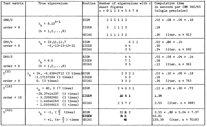
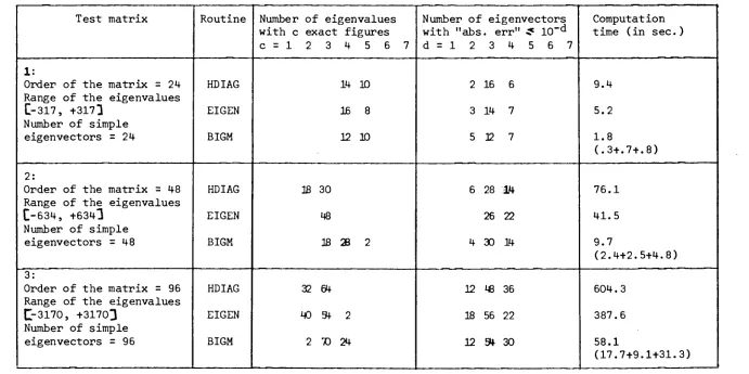
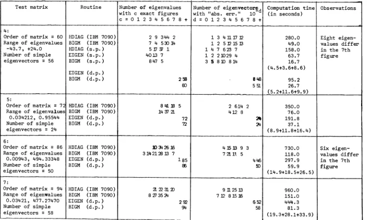
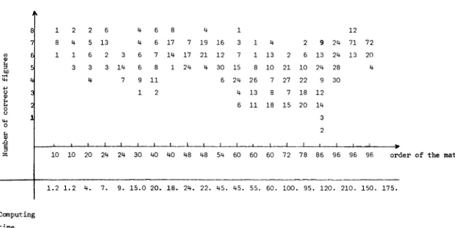
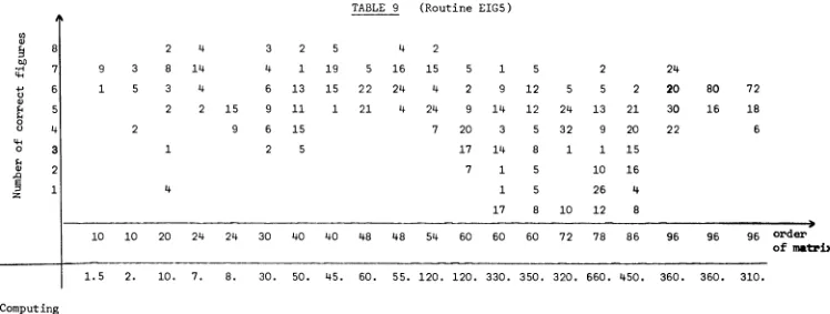
The results of some computational experiments carried out on the above test-matrices are presented in Chapter III. The methods compared for the eigenpro-blem of symmetric matrices are the Jacobi, threshold Jacobi, Givens-House-holder and Rutishauser schemes. The numerical experiments reported in Chapter III §1 give a more realistic picture of the accuracy of the above methods than that obtained by "a-priori error analysis", and make apparent the "efficiency" of the Givens-Householder method for determining the eigen-values of general symmetric matrices. The Rutishauser method is efficient

for determining the eigenvalues of symmetric band matrices.

As far as vectors are concerned the threshold Jacobi method and the Jacobi method give almost exactly orthogonal vectors. The Givens-Householder method

(with inverse iteration) gives accurate eigenvectors, but eigenvectors corresponding to multiple or close eigenvalues may be far from orthogonal.

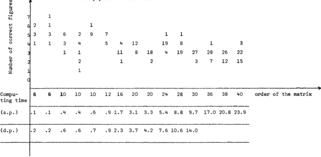
For non-Hermitian matrices the QR method and the Laguerre method are compared. The numerical experiments reported in Chapter III §2 and §3 lead to the follow-ing conelus ion :

a) for finding all eigenvalues, the Laguerre method is troublesome because of the difficulty in finding "convenient" convergence-parameters;

c) the Laguerre method is useful for finding some eigenvalues (especially the eigenvalues with largest modulus) and may be faster than the QR method for matrices with multiple eigenvalues when a convenient choice of the "convergence-parameters" has been made.

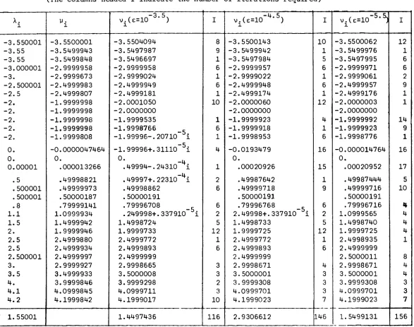
We have considered the iterative method of Wielandt for determining the eigen-vectors of non-Hermitian matrices. The accuracy of each computed eigenvector lying in the linear m-fold subspace spanned by the true eigenvectors which correspond to an eigenvalue of multiplicity m has been tested.

CHAPTER I

A list of test-matrices for the eigenproblem

INTRODUCTION

As test-matrices w usually take matrices which form a representative sample

of those which occur in practice, are general enough as to put sufficient strain on the numerical methods we have to test, and give the solution of the eigenproblem in closed form.

In §1 we give a list of test matrices with known eigenvalues.

In §2 we give a list of special test matrices. Important classes of special test matrices are the unitary matrices, the circulant matrices and the Frobenius matrices.

In §3 the tridiagonal test-matrices are considered.

When we are interested to generate test-matrices with a prescribed distribution of the eigenvalues, it is convenient to resort to matrices generated by

Test matrix SM4/1

4

■2 ­1

0 ­2

4

0

­1

­1 0

0 ­1

4 ­2

­2 4

λ2 = 3

λ4 = 7

Test matrix SM4/2

0.67

0.13

0.12

0.11

0.13

0.96

0.14

0.13

0.12

0.14

0.31

0.16

0.11

0.13

0.16

0.15

Test matrix SM4/3

([l], page 269)

5

■5 5

0

­5 5

16 ­8

­8 16

Test matrix SM4/4

(C1]» Page 302)

0

7

7

21

C\.

=

λ3 =

0.0479716838

0.3111488671

0.6384911230

1.0923883260

λ1 = λ2 = 2·6 5 7 2 8 0 7 3 λ3 = λ^ = 26.34271928

1 1 1

2 3 4

3 6 10

4 10 20

λ = 0.03801601

λ2 = 0.4538345

λ3 = 2.2034461 λ„ =26.304703

Test matrix SM5/1 _[6]

0.81321

­0.00013

0.00014

0.00011

0.00021

­0.00013

0.93125

0.23567

0.41235

0.41632

0.00014

0.23567

0.18765

0.50632

0.30697

0.00011

0.41235

0.50632

0.27605

0.46322

0.00021

0.41632

0.30697

0.46322

0.41931

λ = 1 λ =

2 λ = ₃

λ = 4 λ =

5

-0.29908

0.01521

0.41985

0.81321

4 3 2 1

6 0 0 7 4 6 3 5

4 3 6 5 8 7 7 9

λ = 7 . 5 1 3 7 2 4 1 5 5 λ = 4 . 8 4 8 9 5 0 1 2 0

O

λ^ = 1.327045605 λ^ = -1.096595181

The eigenvectors of the test matrix SM5/2 are:

v^^ Ξ (-0.245877938, -0.302396039, -0.453214523, -0.577177153, -0.556384583)

ν Ξ (-0.550961956, -0.709440339, 0.340179132, 0.0834109534, 0.265435677)

ν Ξ (-0.547172795, 0.312569920, -0.618112077, 0.115606593, 0.455493746)

ν Ξ (0.341013042, -0.116434620, -0.019590671, -0.682043035, 0.636071214)

vc Ξ (0.469358072, -0.542212195, -0.544452403, 0.425865662, 0.0889885036) ο

Test matrix SM5/3

φ.}, page 255)

1 1 1

1 1 1

2 3 4 5

1 3 6 10 15

1 4 10 20 35

1 5 15 35 70

λ = 0.01083536 λ = 0.18124190

λ3 = 1·

λ = 5.51748791 λ^ =92.29043483

Test matrix SM6/1

L

1

1 2 3 0 1 2

2 4 5 - 1 0 3

3 5 6 - 2 - 3 0

0 - 1 - 2 1 2 3

1 0 - 3 2 4 5

2 3 0 3 5 6

λ = 12.41133643 λ2 = 12.41133642 λ = 0.2849864395

Ο

λμ = 0.2849864365 Xc = -1.696322849

ο

λ„ = -1.696322851

ν Ξ (0.170061798, 0.178584630, -0.138066492, 0.295915130, 0.565489671, 0.716086465)

ν3 = (0.669545567, -0.395331735, 0.136726362, -0.288372768, 0.463372193, -0.280810985)

ν Ξ (0.013164189, 0.259286123, -0.199515430, -0.728887389, 0.551154856, -0.240296694)

vc Ξ (0.503951797, 0.074032290, -0.529160563, -0.313202308, -0.521389692, ο

0.300995029)

ν, Ξ (0.391015688, -0.080878210, -0.418685666, -0.446284472, -0.520371701, D

0.441940292)

Test matrix SM6/2 (£l], page 237)

0 1 6 0 0 0

1 0 2 7 0 0

6 2 0 3 8 0

0 7 3 0 4 9

0 0 8 4 0 5

0

o

o

9 5 O

λ

ι

=

λ2 = λ„

=-λ. =

16.60600885 5.94293604 10.06472040 12.12830070 2.10943466 -2.46535845

Test matrix SM6/3

M

253 121 66 11 11 0

121 96 -19 71 -24 7

66 -19 137 -117 73 -14

11 71 -117 152 -82 21

11 -24 73 -82 57 -14

0 7 -14 21 -14 7

λ = λ = 2.533

χ =_{3 4} χ, = 15.618

Test matrix SM8/1

M

611 196 -192 407 -8 -52 -49 29

λ

ι

=

λ2 =

λ3 =

λ4 =

λ6 =

λ7 = λ„ =

196 899 113 -192 -71 -43 -8 -44

1020. 1020. 1019.

λ5 =

-192 113 -899 196 61 49 8 52

04901843

90195436 1000. 0.09804864072 0.0

-1020. 04901843 407 -192 196 611 8 44 59 -23

-8 -71 61 8 411 -599 208 208

-52 -43 49 44 -599 411 208 208

-49 -8 8 59 208 208 99 -911

29 -44 52 -23 208 208 -911 99

The eigenvectors of the test matrix SM8/1 are:

ν Ξ (2,1,1,2, -0.004901843, -0.004901843, 0.009803686, 0.009803686)

v2 Ξ (1, -2, -2, 1, 2, -2, 1, -1)

ν Ξ (2, -1, 1, -2, 10.09901951, -10.09901951, -20.19803903, 20.19803903) O

v4 Ξ (1, -2, -2, 1, -2, 2, -1, 1)

v5 Ξ (7, 14, -14, -7, -2, -2, -1, -1)

νβ Ξ (2, -1, 1, -2, -0.099019514, 0.099019514, 0.198039027, -0.198039027) ν,, Ξ (1, 2, -2, -1, 14, 14, 7, 7)

1 1

1 2

1 3

1 4

1 5

1 6

1 7

1 8

1 1 1 1 1 1

3 4 5 6 7 8

6 10 15 2 1 28 36

10 20 35 56 84 120

15 35 70 126 210 330

21 56 126 252 462 792

28 84 210 H62 924 1716

8 36 120 330 792 1716 3432

λ = 2.2008514614 10

λ = 6.7202144403 10

λ = 8.3730245858 io"

λ^ = 5.1189155425 10

\c = 1 . 9 5 3 5 3 8 7 7 5 4 10C

5 ]

Xc = 1 . 1 9 4 3 1 1 5 5 3 4 10 D

λ = 1.4880477534 IO'

» r

λ„ = 4.5436960082 10e ­3

­1

Test matrix SM8/3

([1], page 239)

a ­b ­c d ­e f g ­h ­b a d ­c f ­e ­h g

­c d

d ­c

a ­b

­b a

g ­h

­h g

­e f

f ­e ­e f g ­h a ­b ­c d

f g

­e ­h

­h ­e

g f

­b ­c

a d

d a

­c ­b ­h g f ­e d ­c ­b a

a = 11111111 e

b = 9090909 f

c = 10891089 g

d = 8910891 h

11108889

9089091

10888911

8909109

8 10 k­1 (k=l,2,...,8)

Test matrix SM8/4

([l], page 244)

Η Κ Μ

Κ Η

Η =

a b e d b a d e c d~~ã E" d e b a

a = b =· c = d = 0 -2 -3 4

Test matrix SM8/5 ([l], Page 238)

33 -3 0 -4 0 8 0 -4 -3 33 4 0 -8 0 4 0 e =

f =

λ = -21

λ2 = λ3 =

λ4 = "5

-13

λ 5 =7

λ6 = λ ? = 11

λ8 = 2 3

6.k ( k = l , 2 , . . . , 8 )

Test m a t r i x SM9/1

_CO

M = (a..) with a.. = a.. = 0 for i t i,i+l and:

3-D 3-D Di­

li 0.71507 0.42721 0.71226 0.42823 0.70177 0.44052 0.43474 0.42862 0.42784

ai+l i=ai i+1 0.13952 0.11389 0.17385 0.021681 0.12899 0.0035016 0.0025372 0.0 0.83818541 0.75787017 0.74734873 0.43584777 0.42784000 0.42773464 0.39554758 0.38360934 0.30227655

Test matrix SM21/1

M = (a. .) with 3-D

η =

CSU

a. . = n+l-i 1 1

a. . = i-n-1 1 1

aii+l = ai+l i »ij = »ji = o

(i = 1,2,. . . ,n+l) (i = n+2,n+3,...,2n+l) = 1

The eigenvalues of M to 7 decimal places are:

λ, = 10.7461942 10.7461942 9.2106786 9.2106786 8.0389411 8.0389411 7.0039522 7.0039518 6.0002340 6.0002175

5.0002444 4.9997825 4.0043540 3.9960482 3.0430993 2.9610589 2.1302092 1.7893214 0.9475344 0.2538058 -1.1254415

Test matrix SM21/2

M = ( a . . ) with ID

η = 10

a . . = n + l - i

1 1

a . . . - — a . „ . — ι ι l + l l + l ι

( i = l , 2 , . . . , 2 n + l )

a . . = a . . = 0 f o r j f i , i + 1 ID Di

The e i g e n v a l u e s o f M t o 7 d e c i m a l p l a c e s a r e :

λ, = +

±

+

+

+

+

10.7461942 9.2106786 8.0389411 7.0039520 6.0002257 5.0000082

+

+

+

+

4.0000002 3.0000000 2.0000000 1.0000000 0.0000000

The eigenvector correct to 8 decimal places of λη = 10.7461942 is:

1.2 A list of real test matrices with known eigenvalues

Test matrix RM4/1

([1], page 228)

-2

1

4

5

Test matrix RM4/2

([l], page 302)

2

-1

-2

-1

Test matrix RM4/3

([l], page 303)

-1

-1

0

o

Test matrix RM4/4

([l], page 303 )

6

9

15

23

-Test matrix RM4/5

( [l] , page 274 ) 1

1

-2

-1

1

5

3

2

3

-1

4

0

1

-3

■12

■23

17119

-50436

49554

-16236

-3

1

5

5

-2

-3

0

-1

0

-2

6

-10

0

1

3

3

2

0

-3

6

1

2

1

3

0

0

-16

18

0

0

1

4

8289 3159

-24326 -9216

23814 8974

-7776 -2! 316

729

-2106

2034

-656

k (k = 1,2,3,4)

Xk = k (k = 1,2,3,4)

λ1 = 2, λ2 = 4

λ3 ' λ4 2 ± 2i

= 7, λ2 = 4

λ3 = 1, \ = -5

λ, = 10 k

k-1

Test matrix RM4/6 ([l], page 237)

9 1 -2 1

1 8 -3 -2

-2 -3 7 -1

1 -2 -1 6

x, = 3.k

k (k = 1 , 2 , 3 , 4 )

Test m a t r i x RM4/7

([13, page 270)

48 -154 176 -64

Test matrix RM4/8 ([£ page 386)

-4 1 -2 7

25 -82 96 -34

5 -1 4 -5

11 3 -37 -10

44 11 -14 - 1

- 1 -7 -4 1

7 -2 1 10

λ = λ = X = 2 1 2 3 \ = 3

λ = % = "Χ = Χ = 3

1 2 3 4

Test matrix RM4/9

0^9612

0.9205 1.0961 0.0677 0.9395

-0.8526 -0.6522 0.2922 0.8977

0.3265 0.8152 0.8561 -0.5330

0.3054 0.3284 -0.1328 0.6556

0.8018 Χ,, λ = 0.0064 + 0.3981 i

o 4 —

The eigenvectors of the test matrix RM4/9 are:

νχ· (-0.1798, 0.3188, 0.9228, -0.1204)

v2 2 ( 0.1890, 0.3465, 0.0309, 0.9113)

Test matrix RM4/10

0

1.31

1.06

2.64

0.07

-0.36

2.86

-1.84

1

0.27

1.21

1.49

-0.24

= 0.03

-0.33

0.41

-1.34

-2.01

3.03

\

= "I·

±i

Test matrix RM5/1

(Ll], page 227)

11

12

-5

3

-2 -6

-11

13

-4

6 5

7

3

7

-2 5

3

-8

5

2 -6

-12

5

-3

7

λ = k k k

(k = 1 , 2 , 3 , 4 , 5 )

Test m a t r i x RM5/2

([1] , page 247)

40

17

-1

13

63 56

10

-6

30

-54

-11

8

6

8

-3 -8

5

5

-19

-3

-39

-17

1

-13

64

Test m a t r i x RM5/3

( [ l ] , page 270)

λ = 1

V

V

1

2

6

-24

120

1

-4

6

■4

1

- 1 1

2 0

0 - 2

-2 0

1 1

- 1 1

- 2 +4

0 6

2 4

1 1

Test m a t r i x RM5/4

_C91

X.

=

λ. =

χ

X

1.50016 + 3.57064 i 1.50016 + 3.57064 i

Test matrix RM6/1

( W . Page 277)

λ 1 7 -6 -1 -8 -4 6 = 3 = 4 3 4 -9 0 3 1 4 -5 2 -1 -5 4 -11 7 2 5 7 ' -11

λ , X

3' 4

Χ , λ

5' 6 -9 -2 1 12 9 1 0 8 2 10 -7 -1

= 1 + 2 i = 5 + 6 i

Test matrix RM6/2 ([1], page 286)

2 4 0 -5 +13 -2 -13 29 -15

0 0 0 0 0 0 5 0 0 -25 61 -48 18 0 0 -36 80 -38 -26 32 -6 -34 24 140 -250 155 -29

*k = k , k = 1(1)6

Test matrix RM6/3 ([1], page 372)

-1 -3 -4 -7 -1 1 -6 -2 16 15 -5 -3 6 3 0 -5 3 3 -14 -7 6 11 -7 -7 21 14 -12 -8 15 7

ίο

1

3 4 7 1 8

\ - \ - i

V

5

V =

6

Test matrix RM6/4 [ β ] ,

\β]

Roots calculated in [ 9 ^ 2.132376 -0.2214068 -0.3184330 10 -0.8983233 10 -0.1706278 10 -0.1394499 io" -1 -3 -4

Roota calculated in Γ83 2.132376 -0.2214066 -0.3184328 10 -0.8983258 io" -0.1706200 10 -0.1443702 IO" -1 -4

Test matrix RM7/1 ([l], page 275)

28 -1 11 -6 -3 14 37 17 29 -1 -11 1 16 -18 -16 7 12 12 -4 -7 -9 11 -6 3 8 3 6 + 5 9 -2 -8 -12 8 2 7 -2 28 10 -5 4 4 26 -27 1 11 6 3 -14 38

k

Test matrix RM7/2 ([l], page 372)

-3 2 -4 0 3 -7 -6 11 3 -1 8 -4 9 9 10 10 1 1 -2 6 4 9 7 2 7 9 0 -5 -13 -16 4 -1 7 -12 3 -2 0 11 -8 7 3 -2 6 -2 4 0 -3 7 9

> 3 =3

Test matrix RM8/1 ([1"3. Page 227)

16 72 79 73 21 73 43 73 17 31 37 -31 -21 -31 -1 31 -11 -53 -56 54 -25 53 39 -53 -17 -59 -55 59 -19 +59 33 -59 -23 -65 -71 65 -60 66 35 -65 29 -13 -7 13 -77 13 43 -13 -19 -61 -67 61 -17 61 42 -60 11 -31 -25 31 -47 31 31 -31 (k=l(l)8)

Test matrix RM8/2 (tl}, page 388)

-7 -1 3 17 9 -3 1 -9

\ , \ ·

_{ι ±}

-9 5 -9 19 8 -8 6 -7 2 i 13 4 -6 4 -1 7 -2 -6 2 -9 -4 3 -6 4 7 8 -12 -1 -13 11 14 -9 -1 -13 -11 8 6 8 4 9 8 -3

V

\

= 3 + 4 i

-13 6 1 9 12 -3 -2 -17 1 -9 5 3 2 7 -10 16

λ , λ

5 » 6 5 + 6 i \ , \_{7' 8 -} = 7+8 i

Test Matrix RM8/3

<EJ» Page

= 2 J

326) -11 -2 -9 3 11 5 -1 -5

:7 i

-23 -9 29 -21 22 2 -22 8

V

λ r

₄

5 + 3 -19 -5 -2 -4 22 4 -8 2 i -13 1 22 -16 12 -8 -11 9

V

Test matrix

([l], page

9 ­

11 5 ­3 1 ­3 ­9 8 16 ■13 6 ­5 9 3 ­1 5 ­1 2 0 7 ­6 2 ­7 4 ­12 5 3 ­2 5 ­2 3 3 ­7 ­4 ­1 ­10 14 ­2 13 ­12 4 ­5 0 ­2 ­13 13 ­6 5 ­6 3 ­2 4 3 0 ­10 ­5 ­3 2 8 7 ­4 1 ­3 1 ­6 ­2 1 ­7 6

λ = k k=l(l)9

Test matrix RM9/2

([ï], page 287)

14 ­91 364 ­989 1886 2509 2236 1210 300 1 0 0 0 0 0 0 0 0 1 0 0 0 0 0 0 0 1 0 0 0 0 0 0 1 0 0 0 0 0 1 0 0 0 0 1 0 0 0 1 0 0 1 0

λ

1 + i

1 + 2 i

Test matrix RM12/1

([1],

page 384)

24 3 4 5 23 8 19 16 3 -2 7 18 3 13 -5 8 40 -9 10 21 5 2 6 -11 -20 -17 7 6 -18 1 13 -4 9 3 -17 -3 10 6 2 -3 26 10 2 +17 -7 -1 6 4 -1 1 12 4 13 -4 1 16 4 12 1 -2 5 -1 5 6 15 -3 0 11 6 5 -1 6 24 12 9 -5 -3 0 -4 -3 -5 9 12 12 -11 4 4 -2 -17 4 2 -20 -2 4 4 -15 16 12 -7 3 -26 -10 -2 -17 7 -4 12 4 40 18 -7 -1 18 -1 -13 4 -4 -3 18 22 -22 -11 1 -13 -17 1 9 -5 -8 0 -8 -7 -29 -3 -4 -5 23 -8 19 16 -3 2 -7 -23

^]r -

± (

I

*)» ± (

I

3")» I

3-,

+

5

1.3 A list of complex test-matrices with known eigenvalues

Test matrix CM3/1

([TJ, page 378)

-189-790 i 537-505 i

438-204 i 361+253 i

-65-144 i 85-115

i

-1626+2740 i

-1788-630 i

-207+581 i

λ =

1+i

λ = 7-8 i

Κ

= -43+51 i

Test matrix CM4/1

([1],

page 251)

12 -(1+i) 2 3(l+i)

-(1-i) 12 (1-i) -2

2 (1+i) 8 -(1+i)

3(l-i) -2 -(1-i) 8

Test matrix CM4/2 ([l], page 287)

2+11 i 3-5 i

6+ 4 i -9+4 i 8-2 i 14- 2 i -30+14 i 22-9 i 25- 8 i -57+28 i 39-24 i

-1+3 i -2+10 i

Xk = (1+i), (3+4 i), (4+5 i), (5+6 i)

Test matrix CM5/1

M

1+ 2 i 43+44 i 5+ 6 i 47+48 i 9+10 i

3 + 4 i 13 +14 i 7 + 8 i 17 +18 i 11 +12 i

21+22 i 15+16 i 25+26 i 19+20 i 29+30 i

23+24 i 33+34 i 27+28 i 37+38 i 31+32 i

41+42 i 35+36 i 45+46 i 39+40 i 49+50 i

λ = 127.387 + 132.278 i O

λ = -9.45999 + 7.28019 i Xc = 7.07332

o 9.55839 i

Test matrix CM5/2

M

-0.845+0.0 i 5.2+0.103 i

5.2 -0.103 i -6.2+0.0 i

0.301+0.0454 -3.39+0.407 i

-9.6 -0.936 i 0.122-0.91 i .0734-7.26 i 4.19+3.66 i

.301-0.0454 i -3.39-0.407 i

0.019+0.0 i .935+0.271 i -0.0572-2.82 i

-9.6+0.936 i .0734+7.26 i +0.122+0.91 i 4.19 -3.66 i

0.935-0.271 i -0.0572+2.82 j 7.21+0.0 i 0.337+0.0603 i 0.337-0.0603 i -1.23+0.0 i

λ1 = 15.180165225 λ2 = 5.6787293543 λ = -0.83398680019

Test matrix CM6/1

íl·

3+i 3 -6+9 i 7i 8-14 i 6-10 i -3-i -3 6-10 i 2-4i -13-5 i -10-5 i -17+3 i - 8+2 i - 8-4 i

-3 -2 -3-i 1-6 i -4 -1+2 i -i

Xk = 0, 1, i, (2+i), (-1-2Í), (-1-2Í)

Test matrix CM10/1 [12]

2+3i 3+2i 5-3i 2+6i l+4i 5-i 5+2i 4-3Í 5+0i 5+2i 3+i -2-i l+2i -2+3i 2+2i 0+4i l+4i 7+3i 2+2i 2+6i l+2i 2+i 3-i 3+7i l+5i 6-5i l+6i l+3i l-3i -l+4i -4+2i l+5i -8-li 8+4i

2-ni

Test matrix CM15/1

([ij, page 278)

Β = C = t 6 20 11 -3 6 9 7 12 12 5 -1 4 10 8

, o

= B+i C 18 28 -6 -15 12 -2 -2 3 5 11 -12 -20 -3 11 5 -2 9 27 5 -1 31 21 7 18 0 2 7 -8 -9 -4 -25 -28 14 33 12 13 5 -4 -4 -1 13 19 3 -18 -12 -10 -12 -33 -9 4 -37 -31 -17 -28 -5 -2 -5 5 -3 -3 20 21 -12 -26 -2 -24 -22 -8 -6 4 -9 -17 -10 13 16 4 6 34 23 -4 18 19 14 19 -2 8 6 -11 -3 0 -28 -24 9 25 10 23 8 3 12 2 8 14 7 -21 -21 -1 -9 -24 -22 9 10 3 0 -3 3 -7 4 8 6 8 40 36 -2 -27 -20 -21 -6 -4 -13 -12 -10 -7 5 33 29 4 16 29 14 -21 -14 2 4 -2 -15 -1 1 -1 -3 -4 -41 -26 12 32 21 27 0 -2 19 13 15 17 5 -34 -38 -5 -15 -30 -21 16 26 11 9 14 10 -6 -2 2 2 -1 19 15 -11 -22 -10 -37 -7 -2 -26 -2 -5 -16 -16 12 23 1 3 24 25 3 -23 -25 -22 -10 9 10 -4 -14 -6 3 -23 -15 11 22 13 41 21 7 23 7 5 16 16 -16 -21 -7 2 -35 -25 -11 -12 3 8 -13 -13 -10 -7 19 0 -14 38 19 -19 -35 -28 -30 -4 5 -13 -15 -15 -24 -12 31 25 18 14 44 21 13 31 9 -5 22 22 14 16 -3 11 14 -36 -25 16 23 4 19 1 -4 12 5 20 30 6 -29 -18 -9 -19 -36 -14 -16 -25 1 15 -12 -17 -11 -16 -2 -2 -3 42 31 -6 -3 16 3 16 18 0 5 -8 -18 7 35 18 22 37 51 27 29 21 -12 -18 9 25 25 32 22 15 5 -52 -36 -3 11 10 8 -8 -13 5 11 9 4 -26 -54 -24 -10 -11 -28 -13 -19 -9 15 23 7 -18 -16 -18 -5 -3 -5 41N 16 -8 -8 -16 -17 1 1 -17 -16 -8 -8 16 41 19

λ

ι

λ4 λ5

λ6 λ7 λ8

CM

= ­5­3Ì

= ­5+2Ì

= ­9+Oi

= ­9+3i

= ­8+5i

= ­4+7i

= 3+i

= 2+4i

16/1

10

S.3

^14

^15

2+8i

3+8i

6+3i

7+2i

3 - 7 i

- 5 - 9 i

9 - 8 i

[12]

( ak i > ( k ; l = 1 , 2 , . . . , 1 6 )

a, . = a , . = 0 f o r 1 i k , k + l k l I k

For k = 1 , 2 , . . . , 1 6

Eingenvalues of A

kk 3+2i ­1­i

3­4i

2+3i

­5+i

l+2i

5+2i

­2+i

l­2i

­l­4i

2+i

l­5i

3+i

2+4i

­4+3i

l­5i

ak ( =

k+1

: ak+l k}

: 4­i

2+4Í

3+i

3­2i

2­2i

2+3i

l+3i

­2+2i

3+3i

­l+5i

4+3i

l­6i

2+i

5­i

­3­4i

0

λ, = +2.06853152 k

2.40341933

2.72491267

2.45640400

2.27740066

0.812811959

­1.38565721

­2.72480368

+1.57598142

+3.28048252

+1.19252750

+3.55339888

­2.45560768

­4.89673115

­5.65716067

5.77408994

­2.05443045Í

+2.08105512Í

­2.37837845Í

+0.631936861Í

+1.44826850Í

+1.33551135Í

­1.38756051Í

+0.657064546Í

­3.83032770Í

+3.27566163Í

­5.44399752Í

+1.26465631Í

­4.69290496Í

+3.62210856Í

+1.63200082Í

§2 SPECIAL TEST­MATRICES

The following procedure can be used for testing methods for solving the non

symmetric eigenvalue problem.

Turning a positive definite symmetric matrix H around its horizontal middle

axis produces a (usually) non symmetric matrix I.H which is similar to a

symmetric matrix M. Indeed it is:

¿>

I =

0

0

0

1 0

0

1

0

0 . . . 0

0 . . . 1

0 . . . 0

0 . . . 0

1

0

0

0

τ

τ

If RR is the Choleski decomposition of Η (Η = RR where R is a lower Τ Λ Τ ­1

triangular matrix) the matrix M = R (IH)(R ) ' is similar to the non

jk Τ* Jk Τ* Τ* 1 Τ1Jk

symmetric matrix IH. The matrix M = R IRR (R ) = R IR is a symmetric

matrix with zero elements below the secondary diagonal. The eigenvalues

of the non symmetric matrix IH are the eigenvalues of the symmetric matrix

ΤΛ Τ

M = R IR, where H = RR , which can be determined by standard methods for symmetric matrices.

Example (Rutishauser):

Η = Pascal matrix of order 5:

1 1 1 1 1

1 2 3 4 5

1 3 6 10 15

1 4 10 20 35

1 5 15 35 70

1

1

1

1

1 0

1

2

3

4 0

0

1

3

6 0

0

0

1

4 0

0

0

0

A IH = M = 1 1 1 1 1 1 0 0 0 0 5 4 3 2 1 1 1 0 0 0 15 10 6 3 1 1 2 1 0 0 35 20 10 4 1 1 3 3 1 0 70 35 15 5 1

1 1

4 1

6 . 1

4 1

1 1 4

3

2

1

0

6 4

3 1

1 0

0 0

0 0

5 10 10 5 1 10 10 5 1 0 10 5 1 0 0

5 1

1 0

o o

o o

o o

The eigenvalues of IH are the eigenvalues of M. The eigenvalues of M

determined by using standard methods for symmetric matrices.

are

2. The test matrices Ai n ) A( n ) [ 1 2 ] , [13]

( η ) ­ ( η ) ­ ( η ) Λ (η) Λ

The Hessenberg matrices A and A have t h e same eigenvalues. A =1 A I A

where I has been defined in 1 ) . det A (n) det Ã( n ) = 1

( η )

η (n­1)

(n­1)(n­1)

0 (n­2)

0 0

0 0

(n­2) .

(n­2) .

(n­2) .

0

0

.. 3

.. 3

.. 3

.. 2

.. 0 2 2 2 2 1 1 1 1 1 1

J(n)

0 .

0 .

3 .

4 .

4 . .. 0

.. 0

.. 0

For n = 12 the eigenw ..ues of A (and à ) are:

λ = .0310280606 λ = 1.5539887091

λη = .0495074292 λ. = 3.5118559486

λ. = .0812276592 λ = 6.9615330856

o y

λ4 = .1436465198 λ = 12.3110774009

λ^ = .2847497206 λ, = 20.1989886459

D 11

Ac = .6435053190 λ = 32.2288915016

The largest eigenvalues of A are very well conditioned and the smallest

very ill­conditioned.

3. The test matrix T( n ) [l^~]

(Algorithm 52):

The elements of the test matrix T of order η are defined by:

T( n ) = (t..) 3­D

t = ­l/c nn

t. = t . = i/c (i = 1,2,...,n­1) in m 2

t.. = (c­i )/c

t±. = t.± = ­ (i.j)/c (i = 2,3,...,n­l; j=l,2,.. .i­1)

where: c = n(n­l)(2n­5)/6

(The n­th row and the n­th column of the inverse matrix (T ) are the

set: l,2,...,n. The matrix formed by deleting the n­th row and the n­th

column of (T ) is the identity matrix of order n­1.

The determinant of T is: det T = t ). All but two of the eigenvalues

( ) n n

of T are unity while the two remaining are given by the expressions 6/(p(n­l)) and p/(n.(5­2n)) where

/3(n­l

y—»

η eigenvalues differing from unity

10 .043532383 ­.083532383

4. The Hilbert matrix H( n )

Elements of the Hilbert matrix H of order n are defined by:

n

H

= (h..)

where h.. = l/(i+j­l) i=l,...,n; j = l,...,n.

(The inverse matrix of the Hilbert matrix is given by:

2

all = n

­ (­l)1+j(n+i­l)!(n+j­l)! 3. . .

i ]

(i+j-l)[(i-l)î(j-l)ï]

(n-i)!(n-j)!

The determinant of the Hilbert matrix is given by:

I*

1!2! ... (2n­l)! det H( n ) = ( 1 ! 2 ! ··· (" ­1 ) ! ) )

The eigenvalues and eigenvectors for Hilbert matrices of order 3 through 10 are

computed in [15Ì.

(4) For example the computed eigenvalues of H are:

λ = 1.500214280059243 10~°

λ = 1.691412202214500 IO­ 1 λ, = 6.738273605760748 IO"3 ­5 λ = 9.670230402258689 10

5) The Eberlein's test matrix E ^n ) [}6~\

E( n ) -= (β..)

s 1]

with: e.. = ­ £(2i+l)n+is­2i J

e.. .. = (i+l)(n+s­i)

e.. = i(n­i+l)

e.. = 0 li­jl > 1

13 1 J 1

s is an arbitrary parameter and (n+1) is the order of the matrix.

The eigenvalues of E are s

λ. = ­j(s+j+l) j = 0,1,2,...,η

In [l6] the corresponding components of the left eigenvectors and of the right

eigenvectors are given.

When s = ­2.­3,...,­2n, the matrix E is defective with two or more pairs

of eigenvectors coalescing. In the range ­2n < s < ­2 at last a pair of

eigenvectors is nearly parallel, and the positive eigenvalues of E are

S

ill­conditioned (especially for s < ­ (n+1)).

6. Brennerb test matrix Β „ Γ17 3

Let Q be the nxn matrix whose entries are all l's. (The matrix Q has rank 1 ) .

The eigenvalues of

B(n> = «I + ßQ α,β

are: α(n­1 times) and α+βη.

The eigenvalues of the matrix

( B ^ f

α,β a+ßn a

are: 1/ct (n­1 times) and 1/(α+βη).

7. Test matrix R

M

The test matrix R (n)

1 1 1 1 1 1 1

­ 1 ­ 2 ­ 3 ­ 4 ­ 5 ­ 6

1 3 6 10 15

­ 1 ­ 4

­ 1 0

­ 2 0

1 5 15

­ 1 ­ 6 1

( TÍ ^ ( n ^ f ­ \ «ρ

The symmetric p o s i t i v e d e f i n i t e t e s t - m a t r i x Ρ

= R

.(R

) with elements

■»■er)

and the matrix ( P( n ))_ 1 = ( R( n ))TR( n ) have the same eigenvalues (R( n ).R( n ) = I),

8. Test matrix L (p)

_t«]

Let η = p­1, where ρ is an odd prime. The elements 1.. of the Lehmer's matrix

T(P>

are:

1. .

3­D

where

e?)·

{*)

is the Legendre­Jacobi quadratic reciprocity symbol, i.e.:

(?)

0 if ρ divides i+j

1 if i+j is congruent to a square, modulo ρ

­1 otherwise.

Example: p=5, n=4.

(5)

­ 1 ­ 1 1 0

­ 1 1 0 1

1 0 1 ­ 1

0 1 ­ 1 ­ 1

(P) ,n­2 rn­2

The eigenvalues of L p are 1, ­ 1 , + J^ (—— times), ­ Sp (—— times),

( \

The inverse matrix of L ^ is the matrix

a

p')

Example :

α ^ Γ

1

^

­3

­1

1

­2

­1 1

3 2

2 +3

1 ­1 ­2

1

­1

­3

fri ì 9

The matrix (L p ) is positive definite with eigenvalues 1 (with multiplicity two) and ρ (with multiplicity (n­2)).

i·

< L

V :

δ..

tf'

9. Frobenius' test matrices F ( η )

The eigenvalues of the nxn matrix

(i,j = 1,2,...,n)

,(n) _

0 1 0 0

0 . 0 . 1 . 0 .

.. 0 . 0 . . 0 . . 1

Pl P2 P3

Pn are the zeros of the polynomial:

. η .n­1 λ ­ ρ λ ­ ρ

1 η r¡

-,η­2

n­1 P l = 0

,(η) .

If F is a non­derogatory matrix (i.e. there is only one Jordan matrix

associated with each distinct eigenvalue λ of F and therefore only one

eigenvector associated with each distinct λ, ) the eigenvector ν corresponding

( "i

to the eigenvalue λ, of F is given by:

_ /,η­1 ­,η­2 . . , Vk ~ k ' k » ··· » AL·» 1'

Frobenius' test matrix F 0 Ό with

n+k-1 Pk = (-1)

has the eigenvalues n-k

n-k+1 )

1,2,... ,n

, (n)> _ . (2k-l)ir.

Since there exists in literature an extensive list of polynomials with known

zeros, the Frobenius matrices are a wide class of test­matriees.

10. Circulant test matrices C (n)

A circulant matrix is one of the form:

,(n) Cl C2 C3 '·· Cn Cn Cl C2 "n­1 C2 C3 C4

and is specified therefore by its first row:

n {c. c„ . . . c} _{1 2 n} ( n )

The e i g e n v a l u e s of C a r e t h e numbers

2 n - 1

λ, = c . + c ζ +c_z + . . . +c z.

k 1 2 k 3 k n k

where z. = cos ( ) + / - l s i n ( ) (k = 1 , 2 , . . . , n ) .

κ η η

The eigenvector of C corresponding to λ, is:

Κ

1 , n­1 n­2 ν

v

k "

r

k '

k "··' V

'

/n

The Brenner's test matrix is a particular circulant matrix of the form C( n ) = {α+β β β ... ß)

,(8)

Test matrix C (C1]' p a g e 2 5 6^

,(8) _ _{{ 1 2 3 4 5 4 3 2}}

λ = λ ­6.82842712

λ3 = \ = λ5 = ° Xc = λη = ­1.17157288

b / λ8 = 24

(16)

T e s t m a t r i x C ( [ l ] , page 240)

,(16)

λ1 = λ2 = λ3 = λ4 = λ5 = λ6 : λ0 = λ = ­26.27414237 λ = λ = ­ 3.23982881

λ = λ = ­ 1.03956613

λ1(= λ = ­ 1.44646269 I H lia

=

= ο

16 80

Remark

Circulant matrices are related to the numerical solution of elliptic and

parabolic differential equations with periodic conditions.

Remark

The eigenvalues and the eigenvectors of block­circulant matrices of order p.m

can be found by computing the eigenvalues and the eigenvectors of ρ sub­matrices

of order m.

(J. Ponstein: Splitting certain eigenvalue eigenvector problems,

Numer. Math. 8, 412 (1966))

11. Unitary test matrices U (n)

The complex matrices U which satisfy the condition

U . LT = Ir .U = 1 (* denotes conjugate transpose)

are called unitary.

Any eigenvalue of U has absolute value 1.

(n) 1 — Test matrix U

2TTk"\

Let rk = e n X (k = 1,2,...,n­1)

The matrix

U<

= A

1

Æ

1 1 ... 1 n­1 1 rx ... rx ι ­p r.n­1

ι r2 ... r2

n­1 1 r ... r

is unitary.

Test matrix U (n)

The nxn real matrix U with elements

ιτπ sin —•Lr

i] V n+1 n+1

U

ij

Vn7T

has Γ-τ-J eigenvalues equal to -1 and (n

12. Test matrix D( n ) (£2(5), page 74)

The skew-symmetric matrix

■Ά eigenvalues equal to +1.

D (n)

O i l - 1 0 1 -1 -1 0

-1 -1 -1

has the following eigenvalues

,(n)

1 1 1

Xk(Dw") = -i cotg ((2k-l) ^ )

(order of D( n ) = n)

(k=l,2,...n).

§3 TRIDIAGONAL TEST-MATRICES

Three orthogonal polynomials with consecutive indices are related by a recursion relation of the form:

Ρ (χ) = (χ-β )Ρ .(χ) - γ Ρ _(χ) η = 2,3... η η n-1 η η-2

Ρ (χ) = 1 _ο

Ρχ(χ) = x­ß1

The polynomial Ρ (χ) can be expressed as the determinant

Ρ (χ) = (­l)n det(J(n)­xI) η

r(n)

ß1

Ύ?

0

0

1 0 0 .

ß2 1 0 . ^ 3 ß3 Χ « 0 0 0

. 0 0

. 0 0

. 0 0

γ Β

η η

Thus the eigenvalues of the tridiagonal matrix J are the zeros of the

orthogonal polynomial Ρ (χ). There are extensive tables of the zeros of the

η ¡ \

orthogonal polynomials £ 2 1 } so that we can consider J and anypolynomial

Ρ(J ) as a test matrix. The inverse (J ) " of some tridiagonal matrices

J are easy to construct ; thus also these matrices have been used for

testing purposes.

Test matrix J( n„ £22 3 o, ß

/ η ) α,β

2+a

- 1

0

0

0 - 1

2

- 1

0

0 0

- 1

2

0

0

0 .

0 .

- 1 .

0

0

. . 0

. . 0

. . 0

2

- 1 0

0

0

- 1

2+β

For la| < 1 and |β| < 1, the eigenvalues of J are: α , β

\

ij

í

n

l· --

2(i

­

cos

ν

where the θ, are the η distinct roots of equation

sin (η+1)θ + (α+β) sin ηθ + αβ sin(n­l)6 = 0

in the range 0 < θ < π.

In particular (k = 1,2,...,η):

, T( n K _ , ,τ( η Κ _ 0 / Λ 2kir.. Xk( J0 , l > - Xk( Jl , 0) - 2 ( 1-C O S 2ηΤΓ)

ι ί τ (η ) ï - ι ( i ^ ï - οΜ „„ο ( 2 k - l ) u ^

Xk( J0 , - l) - Xk( J- l , 0) - 2 ( 1 C O S 2η+1 }

XAJ^h = 2 ( l - c o s ^ T )

k 1,1 η

\ ( J("} , ) = 2 ( 1 - c o s - ^ * )

Κ . ^ Ά

= 2(l-cos - ^ ) = 4 s i n

(

kx 0,0'

n+r

r(n)

iã

The e i g e n v e c t o r s of J~"~ a r e v . , =V—77 sin(——¡-) ( i , k = l , 2 , . . . , n ) ,

f » υ,u I K » n+x n+j. ¡ ν • ν _ determinant of J is equal to n+1. The test matrices (Jn n) and (J ) have the form:

( J( n ))2 ­

(J

o,o

­

Í J( n )i3 ­

( J

o,o) ­

5

­4

1

+14

­14

+6

­1

­4 1

6 ­4

­4 6

1 ­4

­14

+20

­15

+6

­1

1

­4

6

1

+6

­15

+20

­15

+6 1

­4

­4

1

­1

+6

­15

+20

­15

­1 1

6 ­ 4 1

­4 V" 6 ­4 1 ­ 4 5

­1

+6 ­1

­15 +6 ­1

+20 ­15 +6

+6 ­15V +20 ­1 +6 ­15

­1 +6

­1 ­1

­15

+20

­15

+6 +6

­15

+20

-14 ­1

+6

­14

+14

The eigenvalues of (J ) and (J0 j 0) are

>kO

a

»

d

W,

respectively, and their eigenvectors are the same eigenvectors as J (n) 0,0'

Test matrix J (n) a,b,c

T(n) a,b,c

a b 0 0

c a b O

0 c a b

0 0 0 0

0 0 0 0

. 0 0

. 0 0

. 0 0

. a b

. c a

r(n)

The eigenvalues of Jx"' are (be > 0) a,b,c

*kv"a,b,c " " "V *"~ " vn+l λ, (J( n¿ ) = a.­2vTbTÍ cos (­g?)

k a,b.c n+1

-Λη)

Test matrix Jv' (Rutherford, Todd)

-p?q>r

(k=l,2,...,n)

j(n) p>q»r

p­r 2q r

2q r

ρ 2q r 2q ρ 2q r

\

Ν.

r 2q ρ 2q r r 2q p 2q r 2q p­r

(order of J p»q5r

n)

The eigenvalues of J are: (k = l,2,...,n) p,q,r

^ , ( J( n ) ) = (p­2r) ­ - (q2 ­ (q­2r cos k6)2) 6 = ¿SL

k psq,r r ^ n+1

The result has been obtained by relating J to (J . ) . p,q,r a,b,c

The elements a.. of the inverse matrix of J , . are given by:

3­D * » 1 »~1

i(n­i+l)

n+1 for i=j

a..= { a.._ ­i/(n+l)

3­D χ1 1

for j > i

a.. = a. .

D 3- ID

and η is the order of J (n) 2,­1,­1'

for j<i

r(n)

The elements a.. of the inverse matrix of J. , , are given by:

3­D 2,1,­1 B y

Test matrix K

(n)

The inverse matrix of J.

.

has the form:

­*i,u

K

(n)

n

n - 1

n-2

2

1 n - 1

n - 1

n - 2

2

1

n - 2 . .

n-2 . .

n-2 . .

2 . .

1 . . . 2

. 2

. 2

. 2

. 1 1

1

1

1

1

The eigenvalues of K

are:

,(n)

( k = l , 2 , . . . , n )

I n [ 1 3 3 a r e g i v e n t h e v a l u e s of λ (Κ ) f o r η = 12

te = 0.25398978

l¿> - 0.26648096

JUÇ = 0.28918975 yU^ = 0.32555754

Λ5

Λ

= 0.38196601

= 0.47045960

Test matrix Jl

tA

Λ

= 1.3790212

= 2.6180340

= 7.1201222

Λο

Λ ι

ι*12 =63.409139

The tridiagonal Jl^ ­ is related to the Jacobi polynomials.

,

(n)

_ f 2(K+ot­l)(K+ß­l)

«

-ß

.

2K(K+*ié)

1

* / ­ I ( 2K+o(+p­l) ( 2K+*+/S­2 ) '

(2Κ+Α+,β)(2Κ+ο(+/3­2) » (2Κ+ο(+

β)(2Κ+Λ+^­1) J

(Κ = 1,2,...,η)

Text matrix J*

The

e test matrix J

is a particular case of the matrix Jl.

Q

for o*=^=0.

(n)=

(„Κ

'

(J

i *

o,o

·

r

(n)

0

1

1/3

0

2/3

2/5

0

3/5

3/7

0

4/7

<£r>*'­°

r

(n)

(order of J

= n)

The eigenvalues of J

are the zeros of the Legendre polynomials of order η

([21], page 100)

Test matrix J:

r

(n)

(n)

The test matrix J

is a particular case of the matrix Jl

for

d-ß=

..(η) _

(n)

.

,Γ

( J

2

=

­l/2,­l/2

­1/2

r(n)

1

2

2

0

1

1

0

1

0 . 1

1 ^ 0

(order of J. ' = n)

The eigenvalues of J are the zeros of the Thebychev polynomials of first kind:

r

(n).

\(J\

)

= cos(K­l/2)Tl (κ = l,2,...,n)

κ ζ η

(£2f), page 158)

Test matrix J;

r

(n)

(n)

r(n) 1 2

O

1 1

o

1

1

0 1

1 o

1

(order of J*n) = n)

r(n)

The eigenvalues of J3 are the zeros of the Thebychev polynomials of second kind :

(K = 1,2,...,n)

(£24], page 161)

ν ,,(nk _ kW λ (J ) = cos — —

k 3 n+1

Test matrix J2¿

The test matrix J2^ is related to the gemeralized Laguerre polynomials,

J2 (n) ­(K+*­l);(2K+c(­l);

-}

,(n)

The eigenvalues of J2. are the zeros of the generalized Laguerre polynomials,

Test matrix J*n'

The test matrix J n is a particular case of the matrix J2Y1 for <*=0.

1 ­1

­1 3 ­2

r(n) ­2 5 ­3

ν

N.

­(n­2) (2n­3) ­(n­1)

­(n­1) (2n­l)

The eigenvalues of J are the zeros of the Laguerre polynomials of order n

Test matrix J*

o

r

(n)

0

1

1/2

0

2

1/2

0

1/2

v.

(n­2)

0

1/2

(n­1) 0

The eigenvalues of J

are the zeros of the Hermite polynomials of order n

(£21], page 218).

Test matrix J3

(n)

The tridiagonal matrix J3

is related to the Lamé polynomials.

J3

= (a..) i,j = 1,2...n

α

ij

' '

'

a.. = 4(i­l) (1+a)

a

ii+l =

<

" «

a

= ­(2n­2i+4)(2n+2i­3)a

a.

. = 0

3­D

|i­j| > 1

Test matrix J,

£23]

The test matrix J

is a particular case of the matrix J3

for n=13 and

6

α

ai+i i

­540

­534­6

­522

­502.2

­475.2

­441

­399.6

­351

­295.2

­232.2

­162

­84.6

a..

11

0

7.6

30.4

68.4

121.6

190

273.6

372,4

486.4

615.6

760

919.6

1094.4

a· ·_., _{ι l+l}

2

12

30

56

90

132

182

240

306

380

462

552

λ.

1

22.7677122

110.037603

189.702991

261.758027

326.192938

382.990354

432.116798

473.500040

506.948122

531.252512

545.029856

565.168267

592.534780

§4. TEST­MATRICES GENERATED BY KRONECKER OPERATIONS

Let A = (a. .) and Β = (b ) denote NxN and MxM matrices, respectively. The

Kronecker product (tensor product, direct product) of A and B, denoted by

AßB, can be written as N.MxN.M matrix in block partition form:

A®B

a

l l

l 2

*··

i N

2 1

2 2

··'

2 N

a

N l

N 2

··'

N N

If V and W are eigenvectors of A and B with eigenvalues λ and u, respectively,

then VgW is an eigenvector of AfiB with eigenvalue A.y.

The Kronecker sum of A and B, denoted by ΑβΒ, can be written as a (N+M)x(N+M)

matrix in block partition form:

ΑφΒ

A

0

The matrix A<8B has the eigenvalues of A and of

B.

Thus the matrix Α.βΑ„© ... © A has the eigenvalues of A. and of A„,...,

and of A . m

The matrix Α,ΘΑ^φ ... ÖA and the matrix

i ¿ m

Α

ι

0

0

A12 A2 0

0

A13 ' A23 '

A3 '

0

.. A. lm .. A.

2m

" A3m

.. A

m

have the same eigenvalues.

The N.M eigenvalues of the matrix ΑφΙ^+Ι^φΒ are λ.+u. (i=l,2,, , N ; j = l , 2 , . . . , M ) ,

T e s t m a t r i x TP J24]

TP =

A 2A

4A 3A

2irk

Ak( T P1) = 0 . 5 β

2ïïk

W " ^

=0

­

le

0 1 0 0 0

0 0 1 0 0

0 0 0 1 0

0 0 0 0 1

i o "5 0 0 0 0

1 , 2 , 3 , 4 , 5

T e s t m a t r i x TP, [ 8 ]

TP, A

4A 2A

3A

Β = ­2

­3

­2

­1 2

3

0

0 2

2

4

0 A Ξ

2

2

2

5

5B

5B ­Β

Β

Ak(TP2) = 15 + 5 i , - 3 + i , 45 + 1 5 i , 60 + 2 0 i ,

Test matrix TP,

£83

τρ3

=

Β =

8Α

­5Α

4C

­2C 4A

­A

3C

­C

C =

Β

4B 3B

­ 1 1 0

0 0

­ 1 0 1 0

0

­1

" 0 1 0

­ 1 0

0 0 1

­ 1 0

0 0 0

a - l±v­3

λ (TP ) = 3,6,­15,­30,+1.5α, +3α, ±7.5α, ±15α,

4,8,­20,­40,+ 2α, +10α, +20α

Test matrix TP.

£25}

ΤΡΗ =

Β = Α

4Α

6C

8C

­2C

5C 2Α

3Α

­C C

0 C

0 C

­C ­­C

A =

0

2C

2C

C

C = 3B

5B

­2

­3

­2

­1 3B

Β

2 2

3 2

0 4

0 0 2

2

2

5

α = Z+tt , l±2v/:î _{γ = α.}

Àk(TPH) = 120γ, ­40γ, ­24γ, 8γ, 90γ, ­30γ, ­18γ, 6γ, 60γ, ­20γ, ­12γ, 4γ, 30γ, ­ΙΟγ, ­6γ, 2γ

§5 TEST­MATRICES GENERATED BY SIMILARITY TRANSFORMATIONS

We summarize the method of J.M. Ortega £26] for obtaining test matrices

with a prescribed distribution of the eigenvalues. The matrices generated

then the test matrix

S = R + uv*R ­ aRuv* ­ a(v*Ru)uv*

where u and ν are vectors (* denotes conjugate transpose)

_ 1

l+v*u

2 has the same eigenvalues as R. The test matrix S is generated with 0(n )

operations.

For testing accuracy of routines, the matrix S must be generated exactly.

Some special choices of u,v,R facilitate the computation of the test

matrix S.

Symmetric test matrices

n 2

Let Σ v. = 1 , u = ­ 2 v and R = diag(d„d....d ) .

. , ι 1 2 η

i=l

Then

Τ Τ Τ Τ

S = D ­ 2 w D ­ 2 D W + 4(v Dv)vv

is an nxn symmetric matrix with eigenvalues d..,d.,...d and eigenvectors

which are the columns of I ­ 2 w .

In particular, if ν = (η η ...η ) then

Λ { o r n 1

S = ­=r η d.δ.. ­ 2n(d.+d.) + ι+! Σ d, η

2 Ι ι ID

i D

l

k J

(δ., is the Kronecker symbol). 3­D

R e a l and complex t e s t m a t r i c e s

Let R = d i a g í d d . . . d ) , η = 2m, uT = ( 1 1 . . . 1 ) and vT = ( 1 1 . . . 1 - 1 . . . - 1 ) , t h e n t h e e l e m e n t s s . . of t h e t e s t m a t r i x S a r e :

3­D

f d . 6 . . - ( d . - d . + σ) \ ι ID ι ]

i. . = j

1 3 / d.O.. + ( d . - d . + σ) V. ι 13 1 3

1 ^ j \< m

with

n σ ­ L· d, ­ Σ

k=l k=m+"l k

The matrix S is non symmetric with eigenvalues d d ...d and eigenvectors

which are parallel to the columns of I+uv .

If d.(l ­i i <£ η) is a real number the matrix S is a real test matrix (with ι

real eigenvalues). If d.(lí i <? η) is a complex number the matrix S is a

complex test matrix.

CHAPTER II

THE CONDITION NUMBERS OF THE ALGEBRAIC EIGENPROBLEM

INTRODUCTION

Any computing problem is ill­conditioned if the values to be computed are

very sensitive to small changes in the data. A matrix may have some eigen­

values which are very sensitive to perturbations in its elements while others

are insensitive. Similarly some of the eigenvectors may be ill­conditioned

while others are well­conditioned. Besides an eigenvector may be ill­

conditioned when the corresponding eigenvalue is not.

It is convenient to have some number which defines the condition of a matrix

with respect to the eigenproblem and to call such a number the "spectral

condition number''

It is evident that such a single number would have severe limitations. Indeed

if any one of the eigenvalues were very sensitive, then the "spectral condition

number" would have to be large, even if some other eigenvalues were very

insensitive.

A compromise is provided by introducing numbers which govern the sensitivity

of the individual eigenvalues and which are called the "condition numbers

Some relationships between these condition numbers are given. Besides these

numbers are related by inequalities to the "departure from normality", the

"discriminant" of the eigenvalues and the Gram­determinant of the eigen­

vectors of the original matrix.

Finally the ill­condition of the eigenvectors of a matrix is discussed. The

main result is that an eigenvector of a symmetric matrix (which is well

conditioned with respect to the eigenvalue problem) is poorly conditioned

if its eigenvalue is close to the remaining eigenvalues.

When an approximate eigensystem of a matrix has been computed, it is useful

to have some procedure which will give a­posteriori bounds for its errors.

In §6 we summarize some results.

In this report we use the following notations. Τ

The norms of a vector χ (χ = (χ,χ....χ )) are defined by 1 2 η

¡x¡p = (|x1|P + |x2JP +...+ | x JP)1 / p (ρ = l,2,=o)

where ¡xl is interpreted as max Ix.l. _{ι ioo r . ' ι '}

T h e norm j χ| is t h e Euclidean lenght o f t h e vector χ.

T h e matrix norm subordinate t o |x| is denoted by | A | . (A = ( a . . ) . . . ) .

'P 'p ID i,Dsl

η

IA I, = m a x Σ I a..I

1 j i=l 1 ] η

! AI = max Σ la.

ι ι oo

i j=l

I Ax i

¡A| = m a x ι ι ~ = / p ( A * A )

¿ x ¿ 0 i x |2

w h e r e p ( B ) is t h e s p e c t r a l radius o f t h e n x n matrix Β w i t h eigenvalues

λ.λ_...λ .(ρ(Β) = m a x |λ. | ) .

L ¿ Τι . 1 ' „

*

i

*

­

τ

The matrix A is defined b y A = (A) w h e r e A denotes t h e matrix w h o s e elements Τ

are the complex conjugate o f those o f A and Β denotes t h e transpose matrix

o f B. There is a second important norm which is compatible with the vector

norm |x|_. This is t h e so­called E u c l i d e a n o r Schur or Frobenius norm and it is

denoted by ¡A¡ . It is defined by

n n ,2 1/2

A L = ( Σ Σ a.. Γ )

E ·­·. · 1 3.3 '

§1 SPECTRAL CONDITION NUMBER

We consider the "spectral condition number" of a nxn matrix A with respect

to its eigenproblem when A has linear elementary divisors.

In this case there is a non­singular matrix H such that

H_1AH = diagU.)

having its columns parallel to a complete set of right­eigenvectors of A and

such that H has its rows parallel to a complete set of left­eigenvectors

of Α. λ. is the ith eigenvalue of A. Normalized right and left eigenvectors

corresponding to λ. are given by:

­1 Τ

He. (H ) e.

x

i

Turr

*i =

|(H­l)Te.ì

where e. is the ith column of the identity matrix I.

ι J

The number

defines the "spectral condition number" of A.

The overall sensitivity of the eigenvalues of A is dependent on the magnitude

of k(H) since the following theorem holds (£l] , page 87 ; £2])

Theorem (Bauer­Fike)

Let the matrix A be of order η and have η linearly independent eigenvectors

with eigenvalues λ. ( l í i í η). For any fixed matrix B, define the perturbed

matrix Α(ε) = Α+εΒ. Then each eigenvalue λ(ε) of Α(ε) satisfies

min |λ(ε)­λ.I ^ lel IBI Ι Η­11 |H¡

l«i*n P P P

for any p­norm, with ρ = 1,2,°°.

Thus the eigenvalue problem of the matrix A is "ill­conditioned" if k(H) is

"large" (with respect to 1).

When A is an hermitian matrix (A = A ) the "spectral condition number"k(H) = 1;

More precisely the following theorem holds:

If A(e) = Α+εΒ, where A and Β and Α(ε) are hermitian matrices having the

eigenvalues λ., u. and λ.(ε) arranged in non­increasing order, then

|λ.(ε)-λ.| 6 | ε j |B|2 U|e| ( Σ μ ^ )1 7 2)

i=l

An useful bound for the matrix (Λ(ε)­Λ), where Λ(ε) = diag(X.fe)) and Λ = diag(X.),

when A and Β are hermitian matrices is given by the following theorem (£lj,page 104)

Theorem (Wielandt­Hoffman)

If Α(ε) = A+eB, where A, Β and Α(ε) are hermitian matrices having the

eigenvalues λ., u. and λ.(ε) arranged in non­increasing order, than

¡Λ(ε) ­ Λ: £ ^ |ε|·|Β|Ε (=|ε| ( Σ μ2)1 / 2) . i=l

A consequence of the Courant­Fischer characterisation of the eigenvalues of

Hermitian matrices gives the following theorem:

If C = A+B where Α,Β and C are nxn hermitian matrices having the eigenvalues

a., 6. and γ. arranged in non increasing order, then

and

α.+ß ^ Υ, < α. + ß. ι η *" ι ^ ι 1

Σ (γ.­α.)2 ^ Σ β2 = |Β|2

i i

§2 THE CONDITION NUMBERS OF THE MATRIX (WITH RESPECT TO THE EIGENVALUE PROBLEM)

We introduce a condition number which serves as a measure of the effect of

the perturbation of on each eigenvalue of A.

The matrix A has linear elementary divisors; thus Η AH = diag(X.), where

the columns of Η are parallel to a complete set of the right­eigenvectors

of A and the rows of Η are parallel to a complete set of left­eigenvectors

of A.

1

i = 1,2,...η

define the "condition numbers of A" with respect to the eigenvalues λ..

KH'Ve.L I He, I

1 ((Η 1)Tei)1(Hei) x 2 x 2

­1 Τ

We may take the ith column of Η to be χ. and the ith row of Η to be q.y..

With H in this form we have:

H_1(A+eB)H = diag(Xi) + eiq^yTßx. ))?..

= diag(X.) + e(q.$..)?._.

0 1 3. 13 1 3 = 1

T where β.. = y.Bx..

ID Ji 3

An application of the Gerschgorin's theorem shows that the eigenvalues of (Α+εΒ) lie in circular discs with centres (X.+e ß..q.) and radii

Σ | e (q. β..)|. If I b..| < 1, since |B| <£ |B| ■£ n, we have

j^i 1 3.D 13 ¿ h

|β..|« |yj!

|Bx.|

« |B|

|yj|

|x.|

^n .

Thus the ith disc is of radius less than η(η­1)[ε q.¡.

If λ. is a simple eigenvalue of A, for sufficiently small ε he first disc

is isolated and therefore contains precisely one eigenvalue.

If λ is a multiple eigenvalue of A with multiplicity m, there are m discs

with centres X +e q.ß.. (i=l,2,...,m) whose corresponding radii are all

of order e. For sufficiently small e, this group of m discs will be isolated

from the other discs and in their union there are m eigenvalues of A+eB.

When |q.| is "large" (with respect to 1 ) , the eigenvalue problem for finding

X. of the matrix A is ill­conditioned.

1

When A is an hermitian matrix, we have |q.| = 1 for i = 1,2,...,η.

§3 PROPERTIES OF CONDITION NUMBERS

Some relationships between the numbers k(H) and q. are (£l], page 88):

1 « |q. I v< k(H)

1

η

lv< k(H) v< Σ |q.. |