Environmental Kuznets curve (EKC): Times series evidence from Portugal

Munich Personal RePEc Archive

Environmental Kuznets Curve (EKC):

Times Series Evidence from Portugal

Shahbaz, Muhammad and Jalil, Abdul and Dube, Smile

COMSATS Institute of Information Technology, Lahore, Pakistan,

Quaid-e- Azam University, Islamabad, Pakistan, California State

University, Sacramento (CSUS), Sacramento, CA, USA.

15 October 2010

Online at

https://mpra.ub.uni-muenchen.de/27443/

Environmental Kuznets Curve (EKC): Times Series Evidence from Portugal

Muhammad Shahbaz*

COMSATS Institute of Information Technology, Lahore, Pakistan Email: shahbazmohd@live.com

Abdul Jalil

Quaid-e- Azam University, Islamabad, Pakistan Jalil.hanif@gmail.com

Smile Dube

California State University, Sacramento (CSUS), Sacramento, CA, USA. Email: dubes@csus.edu

Environmental Kuznets Curve (EKC): Times Series Evidence from Portugal

Abstract

The paper provides empirical evidence of an EKC – a relationship between income and

environmental degradation for Portugal by applying autoregressive distributed lag (ARDL) to times

series data. In order to capture Portugal’s historical experience, demographic changes, and

international trade on CO2 emissions, we assess the traditional income-emissions model with

variables such as energy consumption, urbanization, and trade openness in time series framework.

There is evidence of an EKC in both the short and long-run approaches. All variables carry the

expected sign except trade openness which has the wrong sign and is statistically insignificant in

both the short-run and long-run. Despite the success of Portugal in containing CO2 emissions so

far, it is important to note that in recent years, emissions have risen. In order to comply with the

1992 Kyoto Protocol on CO2 emissions, there is need for policies that focus on the top five sectors

responsible for about 55 percent of CO2 emissions are due to the extraction of crude petroleum,

manufacturing of refined products, electricity distribution, construction, land transport and

transport via pipeline services.

JEL Classification Codes: C22; E21; P28

Introduction

Empirical evidence on the EKC hypothesis varies from country to country. The results tend to be

mixed when CO2 emissions is the dependent variable, evidence in this paper points to an inverted

U relationship for Portugal. Major contributions of this paper in testing the EKC hypothesis are

threefold. Firstly, we investigate the issue based time series data for Portugal. (Jalil et al. 2010)

suggest that a time series analysis for a single country may provide better framework to study the

relationship. Secondly, the paper employs the ARDL method which is amenable for short time

series data as in this paper. Thirdly, we provide empirical evidence of the EKC by augmenting the

standard GDP variable by trade relationship, demographic factors, and energy consumption (Stern

et al. 1996). Most of the existing literature have used pooled panel data of a group of countries on

the emissions-growth nexus, energy-growth nexus, and emissions-urbanization nexus. These

studies still provide mixed results which is the reason for keeping the problem unresolved.

This paper contributes to the debate on environmental degradation by estimating an EKC for CO2

emissions for Portugal. The rational for selecting Portugal for our analysis is that it has

implemented a variety of programs and policy initiatives that encompass all of the augmented

variables stated above, given that it faces challenges on the environmental front. Portugal has made

great strides in terms of economic growth since its accession to the EU in 1986. The linkages of

energy consumption, trade, urbanization, and economic growth to CO2 emissions have been made

to a greater extent by the 2012 CO2 targets specified under the Kyoto Protocol. As a result,

Portuguese policy makers have focused on reducing greenhouse gas emissions, especially CO2 in

Portuguese economy experienced with 0.90% economic growth rate over the last 2008 year.

However, growth has been associated with structural changes such as the decline in agriculture,

rapid urbanization of coastal areas, and environmental degradation. Despite this impressive growth,

the Portuguese economy faces the challenges in achieving balanced environmental development.

Therefore, the appropriate utilization of resources is important for the environmental protection.

Given this background, Portuguese policymakers have made significant investments and achieved

positive results regarding environmental quality along with the economic growth. These

developments motivate the researchers to investigate the relationship between economic growth

and environmental quality as environmental concerns are making their way into main public policy

agenda.

Economists model the relationship between environmental quality and economic growth in a

variety of emissions-income equations. The objective in these studies is to test the Environmental

Kuznets Curve hypothesis (EKC). The EKC hypothesis suggests that - environmental degradation

increases at initial level of economic growth and then starts to decrease at a higher level of

economic growth. This relationship between measure of environmental degradation, for example

CO2 emissions, and measures of economic growth, for example per capita GDP, is the inverted

U-shaped curve.

The objective of present article is to investigate the EKC for the Portuguese economy over the

period of 1971-2008. In addition to GDP variable, we also include energy consumption, trade and

the urbanization. The rest of the paper consists of: Section II reviews a selected literature

econometric model including the ARDL estimation strategy. The empirical results are reported in

section IV followed by the conclusion and policy implications.

II. Literature Review

An interesting debate prevails over the relationship between environmental degradation and

economic growth in the relevant literature. Most of the studies document the existence of an

inverted-U shaped relationship between economic growth and environmental performance. This is

especially so when other measures of environmental degradation are used. However, when CO2

emissions are the dependent variable, various tests of the hypothesis have produced mixed results.

The growth-environmental performance nexus has been tested by various researchers following the

work of Grossman and Krueger (1991, 1993) and Douglas and Selden (1995). Their work offers

empirical evidence that environmental degradation increases at initial level of economic growth and

then starts to decline at a higher level of economic growth1.

It is worth mentioning here that the different studies tested the EKC hypothesis for different

indicators of environmental degradation, such as deforestation, carbon emissions and municipal

waste. However, sulfur dioxide has been among the most commonly used environmental

degradation indicators and EKC hypothesis has been shown to hold mostly for sulfur dioxide

emissions in the literature (Jalil and Mehmud 2009). Generally, it is difficult to find an inverted-U

form relation for the CO2 emission. A number of studies working on CO2 emissions find an

ever-increasing positive correlation between CO2 and economic growth for example Chang (2010) for

China, Ozturk and Acaravci (2010) for Turkey and Pao and Tsai (2010) for Russia. However,

1

various studies that employ panel data methods report an inverted U-shaped function for CO2

emissions2.

Furthermore, the role of energy consumption in CO2 emission should not be neglected while

discussing the environmental performance and economic growth nexus. A substantial volume of

research has been devoted towards analyzing the energy consumption and economic growth nexus3.

Therefore, researchers think that it will be more fitting if economic growth and energy consumption

is analyzed simultaneously in a single multivariate model (Jalil and Mehmud 2009). This approach

is utilized by Ang (2007), Soytas et al. (2007), Halicioglu (2009), Jalil and Mahmud (2009) and

Shahbaz et al. (2010c) to test both nexus in a single framework.

The next strand in investigating the emission dynamics is to test the relationship between the

dynamics of demographic factors and environmental performance. Shi (2003) and Cole and

Neumayer (2004) found a positive link between CO2 emissions and a set of other explanatory

variables including population, urbanization rate and energy intensity. In addition, few studies have

discussed population density as an additional explanatory variable in the EKC framework (Cole et

al. 1997 and Panayotou 1993, 1995). More recently, Dhakal (2009) examines the relationship

between urbanization and CO2 emissions. In China, evidence indicates that around 40 percent

contribution in CO2 emissions is due to an 18 percent increase in population. Shahbaz et al.

(2010c) investigate the relationship between CO2 emissions, energy consumption, economic

2 _{Heil and Selden (1999), Martinez-Zarzoso and Morancho (2004),Cole (2003),Vollebergh et al. (2005),Galeotti et al.}

(2006)andApergis and Payne (2010b).

3

growth and trade openness for Pakistan. Their results support the EKC hypothesis when energy

consumption and trade openness variables are added to the standard GDP variable. Furthermore,

they find a one-way causal relationship running from income to CO2 emissions. Energy

consumption increases CO2 emissions both in the short and long run, whereas, trade openness

reduces CO2 emissions in the long run.

III. Theoretical and Modeling Framework

The paper follows the framework in Ang (2007, 2008), Soytas et al. (2007), Halicioglu (2009), Jalil

and Mehmud (2009) and Shahbaz et al. (2010c) in estimating an environmental degradation

equation. These studies estimated the emissions-growth nexus and energy-growth nexus in a single

equation model. In addition, we include urbanization as variable to proxy for demographic changes

reflecting the rapid movements of young people from rural and small farms into large cities and

coastal areas in search of jobs. We also include trade openness as a controlling variable. In

equation 1, we suggest that CO2 emission (CO2) in Portugal depend on energy consumption (ENC),

gross domestic product (GDP), square of gross domestic product (GDP2), trade openness (TR), and

urbanization (URB).

(1)

We convert linear specification of model into log-linear specification. It is noted that log-linear

specification provides more appropriate and efficient results as compared to simple linear

functional form of model (Cameron, 1994 and Ehrlich 1975, 1996). Furthermore, logarithmic form )

, , ,

,

( 2

2 f ENC GDP GDP TR URB

of variables gives direct elasticities for interpretations. Therefore, we specify estimable equation in

log linear form:

t URB

TR GDP

GDP

ENCLENC LGDP LGDP LTR LURB

LCO₂ =β₁+β +β +β 2 2+β +β +µ (2)

Whereµ stands for residual or error term, we hypothesize that economic activity is positively

stimulated by an increase in energy use resulting in an increase in environmental pollutants or

energy emissions. This leads us to expect βENC> 0. The EKC hypothesis suggest that βGDP> 0 and

2 GDP

β < 0. The sign of βTR < 0 if production of pollutant intensive items is reduced due to

environment protection laws and imports such items from the other countries where environmental

laws are flexible. The expected sign of trade openness is negative, βTR < 0. Frankel and Rose

(2005) posit that foreign investors come with advanced technology and innovative managerial skills

from their parent country for the advantage of host countries. This tends to increase the use of

energy efficient approaches which further increases welfare. Moreover, trade openness increases in

the demand of environmental quality and cleaner product as trade openness offers a set of available

varieties to consumers (Eskeland and Harrison, 2002). On the contrary, Grossman and Helpman

(1995) and Halicioglu (2009) argue that sign of β_TR is positive if industries of developing

economies are busy to produce heavy share of CO2 emissions with production. Finally, URB

indicates urbanization proxies by urban population as share of total population. Urbanisation is a

variable indicating the demographic growth on environment. A rise in population encourages

population leads to the enhanced energy demand which in turn, creates more atmospheric pollution.

Therefore, we expect β_URB > 0.

The data on all variables comes from World Development Indicators (WDI, CD-ROM, 2009). CO2

emissions is proxied by CO2 emissions (Corban dioxide metric tons per capita), and ENC is for

energy use (kilograms of oil equivalent per capita). Real GDP per capita (GDP) is used to capture

the impact of economic growth on CO2 emissions. TR is for trade openness, which is proxied by

the ratio of exports plus imports to GDP while URB is the urbanisation population as the share of

total population.

IV. Estimation Strategy

This paper applies the ARDL bounds testing approach to cointegration developed by Pesaran and

Pesaran (1997), Pesaran et al. (2000) and latter on by Pesaran et al. (2001) to examine long run

relationship between CO2 emissions, energy consumption, economic growth, international trade

and urbanisation. The autoregressive distributive lag model can be applied without investigating the

order of integration (Pesaran and Pesaran, 1997). Haug (2002) has argued that an ARDL approach

to cointegration provides better results for small sample data set such as in our case, compared to

traditional approaches to cointegration, that is, Engle and Granger (1987), Johansen and Juselius

(1990) and Philips and Hansen (1990). (Laurenceson and Chai, 2003) state that another advantage

of ARDL bounds testing is that the unrestricted model of ECM has sufficient flexibility to

accommodate lags that captures the data generating process in a general-to-specific framework of

orders of ARDL model is sufficient to simultaneously correct for residual serial correlation and

problem of endogenous variables”. The unrestricted model is stated as

t r l n t n o l m t m n l l t l m k k t k q j j t j p i i t i t URB t TR t GDP t GDP t ENC LURB LTR LGDP LGDP LENC LCO LURB LTR LGDP LGDP LENC LCO µ α α α α α α α α α α α α + ∆ + ∆ + ∆ + ∆ + ∆ + ∆ + + + + + + = ∆

∑

∑

∑

∑

∑

∑

The ARDL bounds testing approach to cointegration depends upon the tabulated critical values by

Pesaran et al. (2001) to make a decision about cointegration among the variables. The null

hypothesis of no cointegration in the model isα_ENC =α_GDP =α_GDP2 =α_TR =α_URB =0. The alternative

hypothesis of cointegration among variables isαENC ≠αGDP ≠α_GDP2 ≠αTR ≠αURB ≠0. The next step is

to compare the calculated F-statistics with lower critical bound and upper critical bound critical

values from Pesaran and Pesaran (1997) or Pesaran et al. (2001)4. There is cointegration among

variables if calculated value of F-statistics is more than upper critical bound. If the lower critical

bound is more than computed F-statistics then there is no cointegration. However, if the calculated

F-statistics is between lower and upper critical bounds then decision about cointegration is

inconclusive. In such a situation, we rely on the significance of the lagged error correction term

(ECT) for cointegration to investigate the long run relationship. If a long run relationship among

variables exists, the short run behavior of variables is investigated by the following VECM model:

4 _{For small samples Turner (2006) has assembled critical values for F-statistics that are suitable for the short data series}

t t n s s t m r r t o l l t q k k t p j ECM LURB LTR LGDP LGDP LENC LCO ε η δ δ δ δ δ δ + + ∆ + ∆ + ∆ + ∆ + ∆ + = ∆ − = − = − = − = − =

∑

∑

∑

∑

∑

The existence of an error correction term implies the changes in dependant variable. These changes

are a function of both the levels of disequilibrium in the cointegration relationship and the changes

in the other explanatory variables. This indicates the deviation in dependant variable from a short

span of time to the long-run equilibrium path (Masih and Masih, 1997). The relevance of the

ARDL model is checked through stability tests such as cumulative sum of recursive residuals

(CUSUM) and cumulative sum of squares of recursive residuals (CUSUMSQ).

IV. Empirical Interpretation

Ouattara (2004) states that if a variable is integrated at I(2) then the computation of F-statistics for

cointegration becomes inconclusive as Pesaran et al. (2001) critical bonds are based on the

assumption that such variables should be stationary at I(0) or I(1). Thus, we apply unit root tests to

ensure that no variable is integrated at I(2) or beyond. We have used the ADF unit root test to check

for stationarity. The results in Table 1 indicate that all variables are non-stationary at their level

form and stationary at their first differences.

The two step procedure in ARDL bound testing by Pesaran et al (2001) requires adequate lag

length in variables to remove serial any correlation. The order of lag length has been selected by

estimating firstdifference of the conditional error correction version of ARDL. The selection of lag

calculation of ARDL F-statistics is sensitive to the selection of lag order in the model5. Table 2

shows a maximal of lag more than 2 in the data. The appropriate selection of lag order is necessary

for unbiased and reliable results.

Table 1: Unit Root Estimation

ADF Test at Level with Intercept and Trend

Variable T-Statistics Prob-Value*

LCO2 -0.2961 0.9871

LENC -2.3993 0.3741

LGDPC 0.4353 0.9987

LGDPC2 -0.1559 0.8918

LTR -0.9626 0.9365

LURB -2.2018 0.4715

ADF Test at First Difference with Intercept and Trend

LCO2 -6.8985 0.0000

LENC -6.7119 0.0000

LGDPC -6.8691 0.0009

LGDPC2 -6.7551 0.0000

LTR -5.7913 0.0002

LURB -3.3051 0.0825

Note: *MacKinnon (1996) one-sided p-values

Table-2: Lag Length Selection Criteria

VAR Lag Order Selection Criteria

Lag LogL LR FPE AIC SC HQ 0 140.581 NA 7.31e-09 -7.382 -7.209 -7.321 1 339.1163 343.4125 3.82e-13 -17.25 -16.379 -16.943 2 375.646 55.290* 1.30e-13* -18.359* -16.791* -17.807* * indicates lag order selected by the criterion

LR: sequential modified LR test statistic (each test at 5% level) FPE: Final Prediction Error

AIC: Akaike information criterion SC: Schwarz information criterion HQ: Hannan-Quinn information criterion

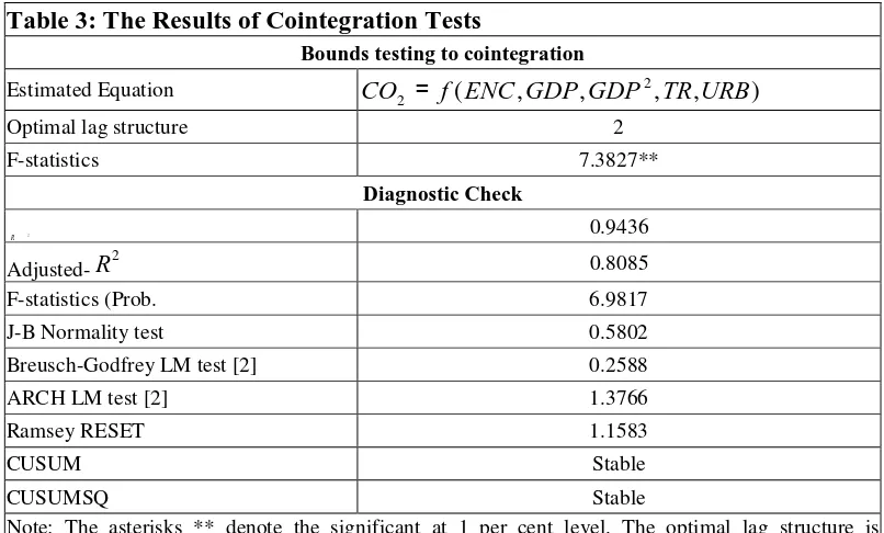
The next step is to calculate F-statistics by ARDL bound test using unrestricted OLS following

equation 3. The results presented in Table 3 indicate a high calculated value of an F-statistic which

is greater than the upper critical bound of 6.198 from Turner (2006)6 at 5% significance. We

conclude that CO2 is cointegrated with ENC, GDP, GDP2, TR and URB when CO2 emissions are

the dependent variable.

Table 3: The Results of Cointegration Tests

Bounds testing to cointegration

Estimated Equation

Optimal lag structure 2

F-statistics 7.3827**

Diagnostic Check

2

R 0.9436

Adjusted-R2 0.8085

F-statistics (Prob. 6.9817 J-B Normality test 0.5802 Breusch-Godfrey LM test [2] 0.2588 ARCH LM test [2] 1.3766

Ramsey RESET 1.1583

CUSUM Stable

CUSUMSQ Stable

Note: The asterisks ** denote the significant at 1 per cent level. The optimal lag structure is determined by AIC.

The long run estimates are reported in Table 4. The results reveal that an increase in energy

consumption increases energy emission or CO2 emissions. For example, a 1 percent increase in

energy consumption raises CO2 emissions by 0.87 percent. This finding is similar to many other

studies on CO2 emissions and energy consumption7. Both linear and non-linear terms of GDP per

6

We have used Tuner (2006) critical values instead of PSS (2001) and Narayan (2005). Turner (2006) produced better critical bounds for small sample data sets.

7 _{See Hamilton and Turton (2002), Friedl and Getzner (2003), Liu (2005), Say and Yücel (2006), Ang (2008),}

Halicioglu (2009), Jalil and Mehmud (2009) and Shhabazet al. (2010c).

) , , ,

,

( 2

2 f ENC GDP GDP TR URB

capita show the existence of inverted-U relationship between economic growth and CO2 emissions.

The coefficients of linear and non-linear terms are 10.25 and -0.57 respectively and are highly

significant.

Table 4: Long Run Estimates

Dependent Variable = LCO2

Variable Coefficient Std. Error T-Statistic Constant -50.9189 9.6869 -5.2564*

LGDP 10.2513 2.1511 4.7655*

LGDP2 _{-0.5736 0.1169 -4.9059*}

LENC 0.8754 0.1379 6.3438*

LURB 0.6020 0.1380 4.3615*

LTR 0.0024 0.0642 0.0380

Diagnostic Checks

R-Squared 0.9948 Akaike info Criterion -3.7678 Schwarz Criterion -3.5030 F-Statistic 1154.062 Durbin-Watson 1.8136 Serial Correlation LM 0.3202 ARCH Test 0.3661 Normality Test 1.0471 Heteroscedisticity Test 1.0063 Ramsey RESET Test 2.6249

Note: * shows a 1 percent level of significance.

The results indicate that a 1 percent rise in per capita income will increase energy emissions by

10.25 percent while the negative sign of squared term corroborates the delinking of energy

emissions and real GDP per capita at high level of income per capita in the country. The evidence

confirms that CO2 emissions increase in the initial stage of economic growth, and eventually

examine the relationship between GDP growth and CO2 emissions8. The coefficient on trade

openness (TR) shows a positive impact on CO2 emissions. The coefficient of TR on CO2 is

positive and statistically insignificant. It indicates that a 1 percent increase in international trade

results in a 0.002 percent increase in emissions. Fossil energy resources are not much available in

Portugal and country imports most of the energy consumed such as oil products due its

consumption structure. Further more, considering domestic demand, both exports and imports are

imputed with CO2 emissions (Cruz, 2004). The coefficient of TR on CO2 is positive, very small

and statistically insignificant. Finally, the impact of urbanization on CO2 emissions is positive and

significant. Urbanization increases energy consumption and hence high energy emissions, resulting

in high CO2. On the basis of empirical evidence, a 1 percent increase in urban population results in

a 0.60 percent increase in CO2 emissions.

Table-5: Granger Causality Test

Null Hypothesis: F-Statistic Pro. Value

LGDP does not Granger Cause LCO2 5.06828 0.03075 LCO2 does not Granger Cause LGDP 0.19584 0.66082

LGDP2 does not Granger Cause LCO2 4.48858 0.04129 LCO2 does not Granger Cause LGDP2 0.18862 0.66673

All variables are I (1), therefore Granger-Causality test can be used to examine the direction of

causality between GDP and energy emissions. The results reported in Table-5 indicate that the

GDP (GDP2) affects the CO2 emissions in the long run. These results also confirm the existence of

Environmental Kuznets Curve (EKC). The evidence is in line with the findings of Zhang and

Cheng (2009) and Jalil and Mahmud (2009) for China, Ghosh (2010) for India, and Shahbaz et al.

(2010c) for Pakistan.

8

The short run dynamics results are reported in Table 6. Evidence indicates that an increase in

energy consumption in the short run leads to increases CO2 emissions. For example, a 1 percent

rise in energy consumption increases CO2 emissions by 0.85 percent. The signs of coefficients of

GDP and GDP2 support the EKC hypothesis and are significant at 10% level of significance

respectively. The impact of a rise in urban population is positive and statistically significant at 5%

level of significance. It implies that a 1 percent increase in urban population will raise CO2

emissions by 0.12 percent. The short run effect of international trade is positive but statistically

insignificant.

Table 6: Short Run Estimates

Dependent Variable = LCO2

Variable Coefficient Std. Error T-Statistic Constant -0.007970 0.017272 -0.461450 LGDP 11.32968 5.986932 1.892402*** LGDP2 _{-0.636843 0.344594 -1.848099***} LENC 0.859039 0.134972 6.364573* LURB 0.120681 0.055179 2.187077** LTR 0.070053 0.060762 1.152896 ECMt-1 -0.108312 0.023200 -4.668681*

Diagnostic Checks

R-Squared 0.8123 Akaike info Criterion -4.0230 Schwarz Criterion -3.7183 F-Statistic 21.6410 Durbin-Watson 1.9832 Serial Correlation LM 0.2401 ARCH Test 0.3234 Normality Test 2.2756 Heteroscedisticity Test 0.5759 Ramsey RESET Test 0.2774

The sign of coefficient of lagged ECM term is negative and significant at 1% level of significance.

This corroborates the established long run relationship among the variables. Furthermore, the value

of lagged ECM term is significant and shows that deviations in CO2 emissions away from long run

equilibrium are corrected by 10.83 percent within a year.

Sensitivity Analysis and Stability Test

The diagnostic tests such as the LM test for serial correlation, normality of the residual term and

White heteroscedisticity test in the short-run model have also been conducted. The results are

reported in Table 4. The relevant statistics show that the short-run model passes all diagnostic tests.

The evidence indicates no serial correlation and the residual term is normally distributed. There is

no evidence of autoregressive conditional heteroscedisticity and the same holds for White

heteroscedisticity. Model specification is well constructed.

Figure 1

Plot of Cumulative Sum of Recursive Residuals

-20 -10 0 10 20

80 85 90 95 00 05

CUSUM 5% Signif icance

Figure 2

Plot of Cumulative Sum of Squares of Recursive Residuals

-0. 4 0. 0 0. 4 0. 8 1. 2 1. 6

80 85 90 95 00 05

CUS UM of S quares 5% Signif icance

The straight lines represent critical bounds at 5% significance level.

The stability tests are used to investigate the stability of long and short run parameters. In doing so,

cumulative sum (CUSUM) and cumulative sum of squares (CUSUMSQ) tests have been employed.

Pesaran et al. (2000, 2001) suggest that CUSM and CUSMSQ tests are adequate in testing for

stability of coefficients in such models. The graph of CUSUM is significant at 5% significance

levels indicating the stability of parameters.

V. Conclusion and Policy Implications

In this present paper, we investigated the relationship among energy consumption, economic

growth, urbanization and energy emissions for Portugal over the period of 1971-2008. The

Environmental Kuznets Curve's (EKC) hypothesis has been tested by applying ARDL model. The

results suggest that a long run relation exists among energy consumption, economic growth,

international trade, urbanization and energy emissions. The existence of an EKC in Portugal

included additional variables that capture demographics (URB), international trade (TR), and

consumption and urbanization on CO2 emissions. Trade openness has positive and significant

impact on CO2 emissions in the long-run.

Since the EKC hypothesis holds in Portugal, we heed Stern’s (1996) warning not to conclude that

economic growth is the means to environmental improvement. Instead, one looks at the trade-offs

among three objectives that have been central in Portugal’s energy policy since its accession to the

EU in 1986; economic growth, environmental protection and energy security. Portugal has made

great strides in terms of economic growth since its accession to the EU in 1986. There is a need for

further policies that address the issue of the total CO2 emissions, 55 percent of which are due to the

top five sectors responsible for CO2 emissions.

However, the 2010 forest fires might have undermined Portugal’s ability to meet 2012 goals. De

Queirozo (2010), reports that The Quercus National Association for Nature Conservation (ANCN)

says that the fires released 1.1 million tones of CO2 this year which they argue reduces “the

capacity of forested areas to absorb carbon, and is a stain on Portugal’s performance under the

Kyoto Protocol.” Similar concerns have been raised about 2010 forest fires by Off7 (a private firm

that certifies emissions). They suggest that a “3% loss of absorptive capacity by forests is

equivalent to 100,000 tonnes of CO2 emissions that the forests were unable to prevent.” If one

considers the fact that in 2008, Portugal’s forest areas absorbed 4.42 million tones of CO2, the

concerns of ANCN and Off7 are significant. Portuguese policy makers need a forestry policy that

has major components namely, zoning, maintenance, management, and regulation of pulp-making

companies. Overall, Portugal’s EKC reflects structural changes of an economy that will have more

decline in CO2 emissions. However, Portugal must have clear policies on clean technologies,

forestry management and increasing rates of urbanization.

References

Abosedra, S., Dah, A., Ghosh, S., 2009. Electricity consumption and economic growth, the case of Lebanon. Applied Energy 86, 429–432.

Ang, J. B., 2007. CO2 emissions, energy consumption, and output in France. Energy Policy 35, 4772-4778.

Ang, J. B., 2008. Economic development, pollutant emissions and energy consumption in Malaysia. Journal of Policy Modeling 30, 271-278.

Apergis, N., Payne, J. E., 2010a. Energy consumption and economic growth: evidence from the commonwealth of independent states. Energy Economics 31, 641-647.

Apergis, N., Payne, J. E., 2010b. The emissions, energy consumption, and growth nexus: evidence from the commonwealth of independent states. Energy Policy 38, 650-655.

Aqeel, A., Butt, M. S., 2001. The relationship between energy consumption and economic growth in Pakistan. Asia Pacific Development Journal 8, 101-110.

Asafu-Adjaye, J., 2000. The relationship between energy consumption, energy prices and economic growth: time series evidence from Asian Developing Countries. Energy Economics 22, 615-625.

Cameron, S., 1994. A review of the econometric evidence on the effects of capital punishment. Journal of Socio-economics 23, 197-214.

Chandran, V. G. R., Sharma, S., Madhavan, K., 2009. Electricity consumption–growth nexus: The case of Malaysia. Energy Policy 38, 606-612.

Cole, M. A., Neumayer, E., 2004. Examining the impact of demographic factors on air pollution. Population and Environment, 26(1), 5–21.

Cole, M. A., Rayner, A. J., Bates, J. M. 1997. The environmental Kuznets curve: An Empirical Analysis. Environment and Development Economics. 2(4): 401-416.

Cole, MA., 2003. Development, trade and environment. How robust is the environmental Kuznets curve? Environment and Development Economics 8, 557–580.

Coondoo, D., Dinda, S., 2008. The carbon dioxide emission and income: a temporal analysis of cross-country distributional patterns. Ecological Economics 65, 375-385.

Cruz, LMG., 2004. Energy use and CO2 emissions in Portugal. Faculty of economics of university of Coimbra (Portugal).

De Queiroz, M. 2010. Portugal’s Forests Losing Ability to Capture Carbon. Inter Press Service, August 31.

Dhakal, S., 2009. Urban energy use and carbon emissions from cities in China and policy implications. Energy Policy 37, 4208-4219.

Dinda, S., Coondoo, D., 2006. Income and emission: a panel data-based cointegration analysis. Ecological Economics 57, 167-181.

Ehrlich, I., 1975. The deterrent effect of capital punishment – a question of life and death. American Economic Review 65, 397-417.

Ehrlich, I., 1996. Crime, punishment and the market for offences. Journal of Economic Perspectives 10, 43-67.

Engle, R. F., Granger, C. W. J., 1987. Cointegration and error correction representation: estimation and testing. Econometrica 55, 251-276.

Eskeland, GA., AE, Harrison., 2002. Moving to greener pastures? multinationals and the pollution haven hypothesis. NBER Working Papers 8888, National Bureau of Economic Research. Feridun. M., Shahbaz. M., 2010. Fighting terrorism: are military measures effective? empirical

evidence from Turkey. Defence and Peace Economics 21, 193-205.

Fodha, M., Zaghdoud, O., 2010. Economic growth and pollutant emissions in Tunisia: an empirical analysis of the environmental Kuznets curve. Energy Policy 38, 1150-1156.

Frankel, JA., AK, Rose., 2005. Is trade good or bad for the environment? sorting out the causality. The Review of Economics and Statistics 87, 85-91.

Friedl, B., Getzner, M., 2003. Determinants of CO2 emissions in a small open economy. Ecological Economics 45, 133-148.

Galeotti, M., A. Lanza., F. Pauli., 2006. Reassessing the environmental Kuznets curve for CO2 emissions: A robustness exercise. Ecological Economics, 57(1): 152-163.

Ghosh, S., 2010. Examining carbon emissions-economic growth nexus for India: a multivariate cointegration approach. Energy Policy 38, 2613-3130.

Grossman, G. M., Helpman, E., 1995. The politics of free-trade agreements. American Economic Review 85, 667-690.

Grossman, G. M., Krueger, A. B., 1991. Environmental impacts of a North American Free Trade Agreement, NBER Working Paper, No. 3914, Washington.

Grossman, G. M., Krueger, A. B., 1993. Environmental impacts of a North American Free Trade Agreement. The Mexico-U.S. Free Trade Agreement”, edited by P. Garber. Cambridge, MA: MIT Press.

Halicioglu, F., 2009. An econometric study of CO2 emissions, energy consumption, income and foreign trade in Turkey. Energy Policy 37, 1156-1164.

Hamilton, C., Turton, H., 2002. Determinants of emissions growth in OECD countries. Energy Policy 30, 63-71.

Haug, A., 2002. Temporal aggregation and the power of cointegration tests: a monte carlo study. Oxford Bulletin of Economics and Statistics 64, 399-412.

He, J., 2008. China's industrial SO2 emissions and its economic determinants: EKC's reduced vs.

structural model and the role of international trade. Environment and Development Economics 14, 227-262.

Heil, M. T., Selden, T. M., 1999. Panel stationarity with structural breaks: carbon emissions and GDP. Applied Economics Letters 6, 223-225.

Jalil, A., Feridun, M., Ma, Y., 2010. Finance-growth nexus in China revisited: New evidence from principal components and ARDL bounds tests, International Review of Economics and Finance 19, 189-195.

Jalil, A., Mahmud, S., 2009. Environment Kuznets curve for CO2 emissions: a cointegration analysis for China. Energy Policy 37, 5167-5172.

Kraft, J., Kraft, A., 1978. On the relationship between energy and GNP. Journal of Energy Development 3, 401-403.

Laurenceson,J., Chai, J. C. H., 2003. Financial reforms and economic development in China. Cheltenham, UK, Edward Elgar.

Lean, H. H., Smyth, R., 2010. CO2 emissions, electricity consumption and output in ASEAN. Applied Energy 87, 1858-1864.

Liu, Q., 2005. Impacts of oil price fluctuation to China economy. Quantitative and Technical Economics 3, 17-28.

Lucas, G., Wheeler, N., Hettige, R., 1992. The Inflexion Point of Manufacture Industries:

International trade and environment, World Bank Discussion Paper, No. 148, Washington. MacKinnon, J G., 1996. Numerical Distribution Functions for Unit Root and Cointegration Tests,

Journal of Applied Econometrics 11, 601-618.

Managi, S., Hibiki, A., Tetsuya, T., 2008. Does trade liberalization reduce pollution emissions? Discussion papers 08013, Research Institute of Economy, Trade and Industry (RIETI). Martínez-Zarzoso, I., A B. Morancho., 2004. Testing for an Environmental Kuznets Curve in

Latin-American Countries. Revista de Análisis Económico 18, 3-26.

Masih, A. M. M., Masih, R., 1997. On temporal causal relationship between energy consumption, real income and prices: some new evidence from Asian energy dependent NICs based on a multivariate cointegration vector error correction approach. Journal of Policy Modeling 19, 417-440.

Narayan, P. K., 2005. The saving and investment nexus for China: evidence from co-integration tests. Applied Economics 37, 1979-1990.

Narayan, P. K., Narayan, S., 2010. Carbon dioxide emissions and economic growth: panel data evidence from developing countries. Energy Policy 38, 661-666.

Narayan, P.K., Singh, B., 2007. The electricity consumption and GDP nexus for the Fiji islands. Energy Economics 29, 1141-1150.

Narayan, P.K., Smyth, R., 2009. Multivariate granger causality between electricity consumption, exports and GDP: evidence from a panel of Middle Eastern countries. Energy Policy 37, 229-236.

Nohman, A., Antrobus, G., 2005. Trade and the environmental Kuznets curve: is Southern Africa a pollution heaven? South African Journal of Economics 73, 803-814.

Ozturk, I., Acaravci, A., 2010. CO2 emissions, energy consumption and economic growth in Turkey. Renewable and Sustainable Energy Reviews. 14(9): 3220-3225.

Panayotou, T. 1995: Environmental degradation at different stages economic development, in Ahmed and J. A. Doelman (eds.), Beyond Rio: The Environmental Crisis and Sustainable Livelihoods in the Third World, London: MacMillan.

Panayotou, T., 1993: Empirical tests and policy analysis of environmental degradation at different stages of economic development, Technology, Environment and Employment, Geneva: International Labour Office.

Pesaran, M. H., Pesaran, B. 1997. Working with Microfit 4.0: Interactive Econometric Analysis. Oxford: Oxford University Press.

Pesaran, M. H., Shin, Y., Smith, R. J., 2001. Bounds testing approaches to the analysis of level relationships. Journal of Applied Econometrics 16, 289-326.

Pesaran, MH., Shin, Y., Smith, RJ., 2000. Structural analysis of vector error correction models with exogenous I(1) variables. Journal of Econometrics 97, 293–343.

Phillips, P. C. B., Hansen, B. E., 1990. Statistical inference in instrumental variables regression with I(1) processes. Review of Economic Studies 57, 99-125.

Reynolds, D. B., Kolodziej, M., 2008. Former Soviet Union oil production and GDP decline: Granger Causality and the multi-cycle Hubbert curve. Energy Economics 30, 271-289. Say, N.P., M, Yucel., 2006. Energy consumption and CO2 emissions in Turkey: empirical analysis

and future projection based on an economic growth. Energy Policy 34, 3870-3876. Shahbaz, M., Lean, HH., Shabbir, MS., 2010c. Environmental Kuznets curve and The role of

energy consumption in Pakistan. Discussion Paper DEVDP 10/05, Development Research Unit, Monash University, Australia.

Shahbaz. M., Ahmad, N., Wahid. A. N. M., 2010a. Savings–investment correlation and capital outflow: the case of Pakistan. Transition Studies Review 17, 80-97.

Shahbaz. M., S M A, Shamim., N, Aamir., 2010b. Macroeconomic Environment and Financial Sector’s Performance: Econometric Evidence from Three Traditional Approaches. The IUP Journal of Financial Economics 1 & 2, 103-123.

Shi, A., 2003. The Impact of Population Pressure on Global Carbon Dioxide Emissions: Evidence from pooled cross-country data. Ecological Economics, 44(1): 29-42.

Song, T., Zheng, T., Tong, L., 2008. An empirical test of the environmental Kuznets curve in China: a panel cointegration approach. China Economic Review 19, 381-392.

Soytas, U., Sari, U., Ewing, B. T., 2007. Energy consumption, income and carbon emissions in the United States. Ecological Economics 62, 482-489.

Stern, D. I., 2004. The rise and fall of the environmental Kuznets curve. World Development 32, 1419-1439.

Stern, D., Common, M., Barbier, E. 1996. Economic Growth and Environmental Degradation: The Environmental Kuznets Curve and Sustainability. World Development 24, 1151-1160. Suri, V., Chapman, D., 1998. Economic growth, trade and the energy: implications for the

environmental Kuznets curve. Ecological Economics 25, 195-208.

Turner, P., 2006. Response surfaces for an F-test for cointegration. Applied Economics Letters 13, 479-482.

Vollebergh, H. R. J., Dijkgraaf, E and Melenberg, E., 2005. Environmental Kuznets curves for CO2: Heterogeneity versus homogeneity. CentER Discussion Paper 2005–25, University of Tilburg.

Wolde-Rufael, Y., 2009. Electricity consumption and economic growth: a time series experience for 17 African countries, Energy Policy 34, 1106-1114.

Yang, H.Y., 2000. A note on the causal relationship between energy and GDP in Taiwan. Energy Economics 22, 309–317.

Yoo, S-H and Lee, J-S., 2010. Electricity consumption and economic growth: A cross-country analysis. Energy Policy, 18 (1), 622-625.

Yoo, S-H., Kwak, S-Y., 2010. Electricity consumption and economic growth in seven South American countries. Energy Policy 38, 181-188.