Munich Personal RePEc Archive
An alternative to portfolio selection
problem beyond Markowitz’s: Log
Optimal Growth Portfolio
Muteba Mwamba, John and Suteni, Mwambi
University of Johannesburg, University of Johannesburg
October 2010
Online at
https://mpra.ub.uni-muenchen.de/50240/
An alternative to portfolio selection problem beyond
Markowitz’s: Log Optimal Growth Portfolio.
Sutene Mwambi
∗and Muteba Mwamba
†Department of Financial Economics/Econometrics
University of Johannesburg
March 10, 2010
Abstract
This paper constructs an alternative investment strategy to portfolio optimization model in the framework of the Mean–Variance portfolio selection model. To differentiate it from the ubiquitously applied Mean–Variance model, which is constructed on an assumption that returns are normally dis-tributed, our model makes two assumptions: Firstly, that asset prices follow a Geometric Brownian Motion and that secondly asset prices are Log-normally distributed meaning that continuously com-pounded returns are normally distributed. The traditional Mean–Variance optimization approach has only one objective, which fails to capture the stochastic nature of asset returns and their correla-tions. This paper presents an alternative approach to the portfolio selection problem. The proposed optimization model which is an optimal portfolio strategy is produced for investors of various risk tolerance, taking into account the stochastic nature of the returns. Detailed analysis based on log– optimal growth optimization and the application of the model are provided and compared to the standard Mean–Variance approach.
1
Introduction to Portfolio Optimization
In this research paper, we construct the growth optimal portfolio (GOP) which is a strategic asset allocation process more suited for those investors with a long term investment view and wish to maximize their expected utility of terminal wealth. Growth optimal portfolio arise from the notion of computing the investment internal rate of return which in essence is bent on constructing those portfolio that have maximal growth. In principle we build a portfolio of risky asset that maximizes the geometric mean.
The paper has primarily been inspired and written in the framework of Modern Portfolio Theory (MPT). Portfolio optimization in the context of portfolio theory is a classical problem in mathematical finance which has spawned a great amount of important academic work. In particular it is one of the well studied classical problems. Central to (MPT) is the Mean–Variance optimization theory(MVO), an important model which was a major breakthrough developed in the 50s and 60s by Markowitz (1952, 1959), his paper opened a new era in the theory of portfolio selection. It plays a important and critical role in determining passive portfolio investment strategies for rational investors and quantifies precisely the relationship between risk and return. His theory set out a way of diversifying investment portfolios so that for any degree of risk, the investor got the best return possible, or alternatively, for any risk, the investor bore the lowest risk. Tobin (1958) built on Markowitz work with the formulation of the “Capital market line” portfolio. Following Markowitz and Tobin, the theory generated a lot of interest and the general equilibrium model capital asset pricing model “CAPM” was independently developed by Sharpe (1964), Lintner (1965), Mossin (1966) .
Markowitz theories pervade the finance industry and are well-known to almost everyone vested in portfolio management. Nonetheless, the Mean–Variance theory suffers from certain well-known draw-backs. The most notable one is that, it is a static optimization problem and is only concerned with
∗Student
solving single period investment strategy hence it can not optimally be applied to any rebalancing pe-riod. Unlike the GOP, it is a strategy that can be applied in multi–period framework and can also be used for any rebalancing period such as a year, a month, a week or a day. However, in our case we investigate the application in a continuous time period. Portfolio rebalancing is also what is commonly known as “volatility pumping”. When volatility is high and a portfolio is rebalanced, an investor would normally yield higher returns. In fact while volatility(risk) is considered bad in static portfolios, it is a positive for growth optimal portfolio.
In order to understand growth portfolios approach, we begin with understanding assets dynamics and how assets prices evolve over time. We characterize that asset behavior follow a stochastic process and can adequately be modeled by stochastic differential equation the “Geometric Brownian motion(GBM)”. Bachelier (1900) was the first to discover that stock prices changes are random and unpredictable. The differential equation has been used in the field of asset pricing see Black & Scholes (1973) because of its unique positivity property. This property of positivity is precisely the nature exhibited in a stock price since stock prices can not be negative but returns can, hence the logarithmic or geometric growth.
The Mean–Variance model requires two model input parameters, thus, the first and second moments and the model is built on the assumption that asset returns are normally distributed Nµ, σ2 and
therefore that the portfolio optimal solution is quantified on the premise that we know collectively the mean vector and variance-covariance matrix. The growth model makes the assumption that continuously compounded asset returns are normally distributed and that price relatives are log–normally distributed a concept which was studied and introduced in financial economics in the late 1950s by Osborne (1959). Campbell, Lo & MacKinlay (1997) outline two remarkable drawbacks of assets returns being indepen-dent and iindepen-dentically normally distributed. Firstly, most financial assets show limited liability meaning that the maximum loss for an investment is equal to the total investment and no more. This implies that the minimum return achievable is−100%1However, normal distribution is defined over the range
[−∞,∞] hence, the assumption of normality clearly violets this lower bound of−100%.
Secondly, if single period returns are assumed to be normal, then multi-period returns cannot be normal since they are simply products of single period returns. In probability theory, the sum of normal single period returns are of course normal, but these sums have no economically meaningful interpre-tation. When analyzing optimal portfolios over longer time periods or on multiple time periods, the normality hypothesis of returns leads to problems. This is because long-term returns are far from being normally distributed. Undeniably, even over a single year, it can be shown that Log-normal distribution, while still not perfect, is a much better approximation to the distribution of the observed historical returns for common financial assets like stocks and bonds see Norstad (2005).
As discussed above, it is quite intuitive to see that asset prices cannot be negative but can only be infinitely positive. It then follows logically that, the investment gross return at any point in time t, 1 +Rt= (SSt−t1) is bounded below. This fact is the basis for suggesting that asset price returns should
be modelled as continuously compounded rt = ln(SSt−t1).
2. The Log-normal distribution often shows a
better fit to historical asset returns as compared to the traditional normal distribution when observed over a longer time horizon. This view is also shared by Palczewski (2005), that asset returns are far from being normal and deviate from the independent identically distribution (i.i.d) assumptions. This formulation is extremely important given both the multitude of areas within economics where portfolio models have found applications and the increasing acceptance of the Log-normality of price relatives in the economic literature.
Any work such as this builds on the advances and ideas of so much knowledge already ascertained in the field and that is this paper is based on the breakthroughs and developments of countless researchers in the fields of finance and statistics and most of all mathematics. Although they are too numerous to name in this space, I acknowledge the foundation that they have built in the field. The remainder of this paper will be elucidated in the next four sections which are described in detail as follows:
1It is easy to see that, since asset prices cannot be negative, the price relative St
St−1 >0. Then by definition the smallest
value thatRtcan have, given that the gross return is 1 +Rt= SSt
t−1 is -100%.
2If gross return is defined as 1 +R t= (SSt
t−1) then taking logarithms on both sides yieldsrt= ln(1 +Rt) = ln(
St
St−1).
This implies thatSt =St−1ert hence the expression ln(SSt−t1) is a representation of a continuously compounded rate of
Section 2 and Section 3 : Introduces literature review and the theoretical background to Log– optimal growth portfolios. The chapter begins the discussion on the central limit theorem and asset dynamics paying particular attention to the Log–normality of asset prices and how the geometric mean relates to simple average returns. It further presents the continuous time mathematics on Geometric Brownian Motion, Ito’s Lemma and the quadratic form of the log–optimal optimization problems. Finally the section deals with the Lagrange multipliers and how the Markowitz quadratic optimization problem is solved using matrix algebra. We study optimization where an investor has more than one risky asset in his portfolio and when a riskless asset is added to a portfolio of risk assets. Finally, the section finishes with the capital market line and construction of tangency portfolio.
Section 4 and 5: The data requirements and test results are presented followed by the research con-clusion. Five stocks randomly selected were used to illustrate how log optimal portfolio are constructed. The data used are the monthly prices downloaded from I-Net bridge, covering the period from the 30 November 1999 up to 31 October 2009. That makes up nine years of monthly data, and in total 120 monthly observations. The assets under consideration were randomly selected from the Johannesburg Securities Exchange namely, BHPBILL, WBHOVCO,NEDBANK,ABIL and SAB and these have been chosen from different economic sectors.
2
Previous work and contribution to existing literature
Over the past 50 years a large number of papers have been dedicated to the Growth Optimal Portfolio (GOP). In financial literature it has been applied in as diverse connections as portfolio theory and gambling, utility theory, information theory, game theory, theoretical and applied asset pricing, insurance, capital structure theory and event studies.
Theoretically, it can be shown that the GOP, which maximizes expected logarithmic utility from terminal wealth, is the portfolio that almost indisputably outperforms all other strictly positive portfolios after a sufficiently long time. Theory has its roots dating back to Benoulli (1954)with the introduction of “expected utility theory” and using the geometric mean as a performance measure of risky portfolios. Kelly (1956) is considered the father of the growth optimal portfolio where in his paper he applied it to the gambling setting. He proposed maximizing the expected exponential growth rate of an investment capital as an investment strategy in a gambling. It is comforting to know that there is a sound theoretical basis for advocating a growth portfolio investment strategy. The Kelly view:that maximizing investment growth of value is a self-evident superior strategy, probably resonates more with the investment sector. However as Christensen (2005) notes that, the first origins of the GOP can be attributed to William (1936). Following, William some remarkable papers on this theory can also be credited to Latane (1959), Hakansson (1971), Elton & Gruber (1974a) and Fernholz & Shay (1982).
The most recent work found on the GOP is by Estrada (2010) with a comparative analysis between the GOP and maximization of the Sharpe ratio. Hunt(2000, 2002, 2005b) attempts to test a simple, practical investment strategy based on portfolios selected to have maximum expected growth rate. Le & Platen (2006) on the other hand applies the theory studying well diversified world stock indices. Elton & Gruber (1974b) argued the practicality of the geometric mean as another alternative portfolio selection criterion in the GOP framework. The development of an algorithm to maximize the geometric mean with assumption log-normally distributed asset prices was entailed by this paper. The methodology was based on the proof that that the maximum geometric mean lies on the efficient frontier in the Mean– Variance space. However, in the conclusion, they pointed out one aspect noting that the construction of the portfolio has major implications for economic theory.
In Weide, Peterson & Maier (1977), it is noted that not much has been documented in terms of finding the optimal solution to the wealth allocation problem of GOP. An investigation into the necessary restrictions under which solutions exist for the case where the retuns distribution is discrete was done. The restrictions were formulated based on the assumption that returnsriare discrete random variables
which can assume a finite numbernof combinations of values.
further pointed out that the GOP model has caused a schism in academia. In some tests it performs well while in other cases the results are rather perplexing. Again it has been shown to outperform the Mean–Variance model but the results are so close due to the operational similarity of the two models.
The effects of long-term out-performance of any strictly positive portfolio by the GOP has been studied, for instance, in Laten (1959). Latane is perceived to be the main scholar in financial economics to have introduced the geometric mean as another approach to portfolio selection criteria and since then the theory has recently received some attention in the academic circles.
Others like, Breiman (1961), Markowitz (1976) and Long (1990) also have made remarkable contri-butions to the theory. In principle, the GOP is the portfolio that cannot be beaten in any reasonable systematic way. Reviews of this portfolio properties can be found in Hakansson & Ziemba (1995) where in their investigation the GOP focused mainly on the relevance of the GOP for investment and gambling setting.
The most far reaching study can be linked to other researchers like Luenberger (1998) and Hakansson (1971) where the use of GOPs on the basis of investors expected utility portfolio maximization was justified. However, the paper compared the Mean–Variance approach to portfolio selection with the capital growth model. A comparison of the two models partly in terms of long-run results may accordingly seem inequitable to the Mean–Variance approach. The reason being that former is a single period model while the later is by definition a multi period model. However, both models are ultimately portfolio models which claim to offer guidance to sensible portfolio choices at any given decision point.
In Platen (2005), the various roles that the GOP plays in finance are discussed and a conclusion is made that the GOP can be interpreted as a fundamental building block in financial market modeling, portfolio optimization and risk measurement and the various ways that the GOP is the best performing portfolio are described. Elton, Gruber, Brown & Goetmann (2003) studied the GOP in the case of a continuous market. No doubt, this property has fascinated many researchers and created a huge and exciting literature on growth optimal investments, a field of study for financial economics.
In Samuelson (1971), evidence for the use of the geometric mean is given and argues, that the law of large numbers or of the central limit theorem when applied to logs can show that a maximum-geometric-mean selection criterion does indeed make it ”virtually certain” that, in a ”long” sequence one will end with a higher terminal wealth and utility, are given. The prescription to select a portfolio that maximizes an investors expected utility is hardly new. Nor are applications in the area of asset allocation. Particularly relevant in this respect is also very recent work by Cremers & Page (2005), and Tim & Kritzman (2007) in which a full-scale optimization numerical search algorithm is used to find an asset allocation that maximizes expected utility under a variety of assumptions about investor preferences. The GOP, however, is unique in that it has dominating characteristics over all other investment strategies.
The determination of the true population mean and variance-covariance matrix is indeed a signifi-cant part to the entire optimization problem. In order to estimate the expected portfolio return, the Mean–Variance methodology uses historical data on the assumption that the sample mean is a true rep-resentation of the population mean. The sample mean and sample variance are simply average values of a finite data sample, and are not entirely true representation population parameters. As a consequence of that, it is imperative that we revisit how we parameterize the Mean–Variance model. In addition, due to the amount of volatility in asset returns,sample means may not provide accurate estimates of the true population means. As a consequence, utilizing the sample version into a model expecting the population equivalent can produce off-the-wall results. In particular, an investor could be inclined to invest large amounts of money into securities and sectors that performed better than expected in the past.
3
Methodology: Log Optimal Portfolio Selection Criterion
As a preamble to understanding the growth optimal portfolio, we start by introducing the theory on the geometric mean followed by a background to the mathematics of continuous time processes underlying stochastic variables.
3.1
Geometric Mean and Asset Prices as Random Processes
In an investors wealth perspective, the growth of the asset over the entire period [0, T] should be expressed as a geometric mean. The use of geometric mean has far better properties in terms of the interpretation of asset returns as compared to the arithmetic mean. In analyzing wealth over a longer period of time, the geometric mean conveys what the average financial rate of return would have been over the whole duration of the investment period.
Combining the results discussed in the previous section, whereRt= SSt−t1−1 represents price return
for a single period, between dates t−1 andt. Then for n single periods returns, a sequence of asset returns defined as{Rt}nt=1 based on the sequence of asset prices{St}nt=0, the geometric mean return or
the so-called “time-weighted rate of return,”r(0,n), can be expressed as follows:
r(0,n)=
n
Y
t=1
(1 +Rt)
!1
n
−1. (1)
There is, however, a mathematical relationship between the geometric mean and the arithmetic mean of logarithmic returns. The geometric mean can technically be viewed as an average of logarithm values of asset returns. Thus:
n
Y
t=1
(1 +Rt)
!1
n =e
1
n
Pn t=1ln
“
St St−1
”
. (2)
However, this also implies that,e
1
n
Pn t=1ln
“ St
St−1
”
=e
1
nln
“
Sn Sn−1
Sn−1
Sn−2···
S1
S0
”
and this represents the expres-sionSn
S0
1
n
. Hence from equation [2] we have lnSn
S0
= ln (Qnt=1(1 +Rt)).This equation implies that
the geometric mean is just a function of the mean of the log-returns3, if they are interpreted as statistics,
that is:
r(0,n)=eE
h
ln“St−St1”i
−1, (3)
from the above equation, we can therefore infer that the objective of the Growth Optimal Portfolio (GOP) rests in maximizing the mean (Gmax) which is the same as maximizing the mean of the log-returns due
to the monoticity of the exponential function, thus:
Gmax= max
E
ln
St
St−1
, (4)
whereEis the expectation operator.
Now let {Rt}nt=1 be a sequence of independent and identically distributed (i.i.d.) random variables
with finite mean and variance, then so is the sequence:{Zt|Zt= ln (1 +Rt) andt∈1,2,· · · , n}.Then it
is clear that,lnSn
S0
=Pni=tZt.Choosing a time horizon T and letting△t=T /n, we demonstrate the
distribution dynamics of lnSn
S0
. First we look at the Central Limit Theorem (CLT) which says that: Theorem 3.1. [Central Limit Theorem]Let random variablesY1, Y2· · ·,be independent and identically
distributed with finite mean µ and variance σ2 generated from any distribution. Then as the sample
sizes gets large, the sampling distribution of the mean approaches a normal distribution with meanµand variance σ2/N.
3This is stated more formally in the textbook by Luenburger, D. (1998), page 420, were the rationale for the result is
Having the CLT in mind and thatE(Zt) =µ△tandV(Zt) =σ2△t, then lnSn
S0
/nis approximately normally distributed:
lnSn
S0
n ∼N
µ△t, σ2△t
n
. (5)
Hence, lnSn
S0
∼N µT, σ2T. Another way of expressing this is in the form lnSn
S0
=µT +σ√T ǫ.
where ǫ has a standard normal distribution. In particular, it is not an unreasonable assumption to assume that theZtabove are normally distributed i.i.d. and then we have that (by definition),
ln
St
St−1
=Zt=µ△t+σ
p
△tǫt, (6)
which is by definition just the discrete random walk,ǫtbeing just a sequence of standard normal variables.
Note that by the following theorem on random variable transformation;
Theorem 3.2. [Transformation of random variables] Let X be a continuous random variables having probability density function fX. Suppose g(x) is strictly monotone, differentiable function of x. The
random variable Y defined by Y =g(X)has probability density function given by
fY(y) =
fX
g−1(y) d
dyg−
1(y) if y=g(x)for somex,
0 if y6=g(x)for all x,
we have that,Sn
S0 ∼Log-normal µT, σ
2Twhich is an important result showing that price relatives
are log-normally distributed, given the assumptions above.
3.2
Geometric Wiener Process
We have so far given a thorough introduction to asset dynamics and specifically the stochastic process of how asset prices change over time in discrete terms. Having said that, this section provides a more rigorous approach to asset behavior in continuous time mathematics. We now formalize the stochastic growth model for the optimal portfolio selection optimization problem. In continuous time mathematics, the log normal random walk model in equation for non dividend paying asset is usually formulated in terms of the following stochastic differential equation.
dlnS(t) =µdt+σ√dtǫt. (7)
Where the parameters µand σrepresent percentage drift rate or instantaneous rate of return and the percentage rate of volatility respectively. The two parameters could be constant or could depend on the stock price and/or time. The term√dtǫtis the standard wiener process whereǫt∼N(0,1), the process
represents something like the infinitesimal stochastic change in lnS(t) over an infinitesimal instant of time. It then follows that, µdt+σdw(t) ∼ N µdt, σ2dt, hence dSS((tt)) ∼ N µdt, σ2dt. Equation [7] cannot be interpreted as an ordinary differential equation, since the Brownian paths √dtǫt are not
differentiable with respect to time. It was precisely for the purpose of dealing with differential equations incorporating stochastic differentials that It¯o developed what is now called the It¯o calculus. The left hand side represents the percentage change in asset value and it equivalent to stating it asdlnS(t) = dSS((tt))4,
substituting the expression into equation [7], we obtain the following expression,
dlnS(t) = dS(t)
S(t) = µdt+σ
√
dtǫt. (8)
⇒dS(t) = µS(t)dt+σS(t)√dtǫt. (9)
which is the It¯os diffusion process, now let√dtǫt =dw, It¯os lemma states that for the process above
and a function F(S, t) which is twice continuously differentiable in both S and t then, the change in
F(S(t), t),dF(S(t), t) is also an It¯o process, subsequently,
dF(S, t) =
∂F
∂SµS+
∂F
∂t +
1 2
∂2F
∂S2σ
2S2
dt+∂F
∂SσSdw. (10)
We know thatS(t) follows the process defined by equation [9]. Then, the process followed bydlnS(t) can easily be solved by defining a function F(S(t)) = ln (S(t)) and since this is a function of only S
and nott, then the It¯o lemma takes the formdF = µSF′+1
2σ2S2F′′
dt+σSF′dw. Applying the It¯o
lemma, we derive the governing process outlined byF(S(t)) = lnS(t).Then, the process followed bydF
is
dF =
µ−12σ2
dt+σdwt where dF is representing dlnS and dwtis
√
dtǫt
(11) Equation [11] concludes thatdlnS follows the Wiener process. 5
Integrating and set the initial value conditionF(0) = lnS(0) yields;
F(t) =F(0) +
Z t
0
µ−12σ2
ds+
Z t
0 σdw
=F(0) +
µ−1
2σ
2
t+σw(t).
We know that F(s) = lnS then,
lnS(t)−lnS(0) =
µ−1
2σ
2
t+σw(t)
ln
S(t)
S(0)
=
µ−1
2σ
2
t+σw(t)
S(t) =S(0)e(µ−12σ 2
)t+σw(t), (12)
discretized, this can be written as:
St=St−1e(µ−
1 2σ
2
)△t+σǫ√△t. (13)
In essence we are stating that stock prices follow a Geometric Wiener process and that over any time increment, △t, the distribution of logarithmic returns is normally distributed with mean α△t, where
α= µ−1
2σ
2, proportional to the time increment and the volatility,σ√
△tis proportional to the square root of time increment.
The probability distribution function of X= lnSS((0)t)∼ N µ−12σ2t, σ2tis;
f(X) = √ 1
2πσ2te
−1 2
"
X−(µ−12σ 2)
t σ√t
#2
(14)
and through Jacobian variable transformationY =eX=elnStS0 =e(µ− 1 2σ
2
)t+σtis lognormally distributed
with parameters µ−1 2σ
2tandσ2t. ElnSt
S0
= µ−1 2σ
2tand the variance is,VlnSt
S0
=σ2t
This statement stated differently is saying that the the change in asset prices when modelled using the Geometric Brownian motion are log-normally distributed. Applying theorem 3.2, the probability density function ofY is as follows;
5notice that the left hand side is a expression of the forma+bxand ifx∼N(0,1) theny=a+bx∼ N`
a, b2´
. Hence
dlnS∼ N“`
µ−1
2σ2
´
f(Y) = 1
y√2πσ2te
−1 2
"
lny−(µ−12σ 2
)t σ√t
#2
(15) Putting all the pieces of information discussed so far together, we conclude that the Geometric Brownian motion is lognomally distributed thus,
St
S0 ∼
LN
µ−12
t, σ2t
and
The expected valueESt
S0
=Ee(µ−12σ 2
)t+1 2σ
2
t=eµt
If we put all the pieces of information discussed so far, then, by employing the GBM to estimate the model input parameters, we significantly change the whole Markowitz’s setting and in particular we construct a portfolio which maximizes the expected growth rate hence the name Log-Optimal growth portfolio. The methodology of how this is achieved is the topic of our discussion the last chapter.
3.3
Log Optimal Portfolio Selection Criterion
We also focus on the key analytic tools employed in portfolio optimization methods where we introduce the elements of stochastic calculus as an important tool in modeling of financial processes, see Wilmott (2001) for a detailed introduction on the subject of SDE6. We further review the standard analytic
approach based on mean-variance assumptions and then describe a more general procedure that assumes investors seek to maximize expected utility. We will show, later, that mean-variance procedures are special cases of the more general expected utility formulations. We term the more general approaches Expected Utility Optimization and the traditional methods Mean-Variance optimization.
The problem dealt in this paper realistically deals also with the problem of rebalancing the portfolio in any time horizon. In small time horizons, the portfolio rebalancing a log optimal growth portfolio is constructed as a as continuous-time stochastic process.
Suppose an investor has a choice of investing in a finite number of correlated risky assets represented by ann×1 vector S= [S1, S2,· · ·Sn] where, without loss of generality, it can be assumed that each Si
represents the asset and its price. Then, for each asset{Si}ni=1, the price is assumed to be governed by
a Geometric Brownian Motion:
dSi
Si
=µidt+σidwt,wherei∈ {1,2, . . . , n}. (16)
By our earlier assumption, the assets prices are correlated through the Wiener process dwt=ǫi
√
dt
with a probability density function fdwt(x) =
1
√
2πdte−
x2
2dt and the covariance, Cov [dwi, dwj] = σijdt whereσij can be understood as the correlation between assetsiandj. In the Markowitz framework the
Wiener vector,dw= [dw1, dw2, . . . , dwn] has a multivariate Gaussian distribution hence,
fdw(x1, . . . , xn) =
1 (2π)n2
|Σ|12
e[−12(x−µ)′Σ− 1
(x−µ)]
. (17)
The vector µ is just the zero vector since ǫi
√
dt ∼ N(0, dt), |Σ| is the determinant of the covariance matrix Σ, and then×ncovariance matrix is defined having diagonal elementsσ2
idt,fori=j andσijdt
fori6=j. The symbol e is an exponential function representing the number approximately 2.7182818 In the multivariate framework we have the log price change for time (t−t0) from the univariate
solution in equation [12] as normally distributed, lnSi,t∼N
lnSi,t0+
µi−
σ2
i
2
(t−t0), σi2(t−t0)
. (18)
The asset prices at some future deterministic date (t), given that we know the asset price at time (t0) is
lognormally distributed and the standard deviation is proportional to the square root of the time interval of how far ahead we are looking. From Equation [18] we have:
E
ln
S
(i,t) S(i,t0)
=
µi−
1 2σ
2
i
(t−t0) And the variance isV
ln
S
(i,t) S(i,t0)
=σ2
i(t−t0).
Let the sequence of portfolio weights be denoted{ωi}ni=1, such that Pn
i=1ωi= 1 represent the budget
constraint. The overall portfolio valueP can be formulated in terms of the aforementioned stochastic processes as follows:
dP
P =ω1
dS1
S1
+ω2
dS2
S2
+· · ·+ωn
dSn
Sn
=
n
X
i=1 ωi
dSi
Si
=
n
X
i=1
ωi(µidt+σidwi). (19)
One thing to note is that the portfolio is a weighted sum of the assets.
In continuous time, the percentage change in the value of our portfolio, is normally distributed with mean:
E
ln
Pt
Pt0
=
n
X
i=1
ωiµi(t−t0)−
1 2
n
X
i,j=1
ωiσi,jωj(t−t0); (20)
and the portfolio variance is:
V
ln
Pt
Pt0
=
n
X
i,j=1
ωiσi,jωj(t−t0). (21)
3.4
Deriving the Weights that Maximize Portfolio Growth Rates with Short
Selling Allowed
Fornassets with linearly independent growth returns, a portfolio of risky assets modelled in continuous time has a growth rate ν = 1
(t−t0)
EhlnPt
Pt0
i
= ω′µ−1
2ω′Σω. Denote µ =ν + 1
2ω′Σω as a column
vector representing the expected growth rates, let Σ denote the variance-covariance matrix of the growth rates and ω represent a column vector of portfolio weights which are chosen to maximize the growth rateG. Letθ= 1 be the risk aversion parameter this equal to a unity since it does not affect our finale solution. In the Markowitz framework the portfolio optimization problem entails minimizing the portfolio variance for some specified portfolio mean. However the duplex to the problem, is the maximization of the portfolio growth for some specified portfolio mean- the GOP problem. Symbolically the the two problems are formulated as follows;
argmin
ω
θ
2ω
′Σω |ω′µ=E(Rp) ω′e= 1
(22) argmax
ω
ω′µ−θ
2ω
′Σω |ω′µ=E(Rp) ω′e= 1
. (23)
whereRp in the portfolio return defined in the following way: E(Rp) =Pin=1ωiE(Ri) andRi is the i-th
asset return, andeis a column vector of ones. Notice that the risk aversion parameterθ
3.4.1 Minimizing the Portfolio variance(σ2
p =ω′Σω) for a Specified Mean E(Rp)
Definition 3.1. A portfolio,P, is the minimum variance portfolio of all portfolios with mean returnµp
if its portfolio vector of weightsω is the solution to the following unconstrained optimization problem,
argmin
ω
n
2ω′Σω |ω′µ=E(Rp) ω′e= 1
o
. (24)
The Lagrangian function with λ and γ as multipliers is constructed for the optimization problem above, hence:
L=ω′Σω
2 −λ[ω′µ−µp]−γ[ω′e−1]. (25) We optimize the Langrangian by differentiating with respect toω,λandγ and set the derivative equal to zero to yield these three sets of matrix equations:
dL
dw = Σw−λµ−γe= 0, (26)
dL
dλ = w
′µ−µ
p= 0, (27)
dL
dγ = w
′e−1 = 0. (28)
Solving forω, notice that we can rewrite the first equation as follows,
ω= Σ−1[λµ+γe]. (29)
Recall from the equations in 26 that dL
dγ =ω′e−1 = 0, then by substitution, we have an equation of the
form,
λµ′Σ−1e+γe′Σ−1e= 1. (30)
Similarly, we know thatµp=ω′µ, hence
µp=λµ′Σ−1µ+γe′Σ−1µ. (31)
In order to get the closed form solution forλandγ we solve a system of two simultaneous equation(30 and 31),
µp
1
=
λµ′Σ−1µ+γe′Σ−1µ
λµ′Σ−1e+γe′Σ−1e
. (32)
The system above can be represented in a more elaborate matrix form as follows:
µp
1
=
µ′Σ−1µ e′Σ−1µ
µ′Σ−1e e′Σ−1e
λ γ
. (33)
Notice in Equation 33 thate′Σ−1µ=µ′Σ−1e, then the expression can be simplified to:
µp
1
=
A B
B C
λ γ
, (34)
where we define:
A=µ′Σ−1µ, B=µ′Σ−1eandC=e′Σ−1e.
A closer inspection of all the entries in the matrix above reveals that they are scalars. Also notice that the equation is a linear system of the form Λx=b, so solving for this system would be asx= Λ−1b:
From the inverse of the matrix, thus solving for the two unknown multipliers γandλwe get,
λ γ
= 1
AC−BB
C −B
−B A
µp
1
Multiplying out the expression we get:
λ= Cµp−B
AC−BB and γ=
−Bµp+A
AC−BB.
Finally putting all the pieces together we write down the solution forω which will be a n×1 vector of portfolio weights as follows:
ω∗= Σ−1[λµ+γe]
= 1
DΣ−
1[(Ae
−Bµ) +µp(Cµ−Be)]. (36)
The equation of the minimum variance set of the portfolio can then be shown to be
σ2p=ω′Σω=λµ
p+γ,
= Cµ
2
p−2Bµp+A
AC−B2 . (37)
The portfolio variance is a quadratic function of the mean portfolio return. In the (µp, σp) space this
plots the parabola while in the (σp, µp) space this plots the inverted parabola. The global minimum
variance portfolio (gmv) has the mean return which is found by differentiating the equation for the variance and setting the derivative equal to zero d(σ
2
p)
dµp =
2Cµp−2B
AC−BB = 0. This yields µ
gmv
p =BC which
simplifies to the following,
Mean of Global Minimum Variance =µ′Σ−
1e
e′Σ−1e, (38)
It is easy to see that the variance of the GMV portfolio σ2 gmv =
CB2
C2−2B
B C+A
AC−BB and further algebraic
manipulation this can be expressed as follows:
Minimum Variance = 1
e′Σ−1e. (39)
The portfolio weights for the global minimum variance portfolio (gmv) can also easily be computed from Equation [36] by substitutingµp for BC. This givesω∗= Σ−1
µ(CB
C−B)+e(A−BBC)
AC−BB
and the weights are therefore equal to the following,
Portfolio Weights of the GMV = Σ−
1e
e′Σ−1e.
3.4.2 Maximizing the Log-Optimal Growth portfolio for a Specified MeanE(Rp)
In the GOP framework, we demonstrate the similarity with the weights of both the GOP and the Mean– Variance optimal weights. Solving for the optimal solution to this problem is similar to the problem above and a complete derivation is outlined in appendix B. The Lagrangian is therefore,
L=ω′µ−ω′Σω
2 −λ1[ω
′µ−µ
p]−γ1[ω′e−1] (40)
It is easy to show that
ω= Σ−1[µ−λ1µ−γ1e].
Hence, the system above can be represented in a more elaborate matrix form as follows
µ′Σ−1µ−µ
p
e′Σ−1µ−1
=
µ′Σ−1µ e′Σ−1µ
µ′Σ−1e e′Σ−1e
λ1 γ1
therefore the optimal weights are given as λ1 = CXD−BYandγ1 = AY−DBX, where D = AC−B2 and
X =µ′Σ−1µ−µ
p andY =e′Σ−1µ−1. Hence, the weights are given as.
ω∗= Σ−1µ−CXD−BYΣ−1µ−AY −DBXΣ−1e. (42)
The results display a remarkable similarity between the log optimal and mean variance optimization problem as is evident from equation [42] which is identical to equation [36]. This can be shown as follows; To show that the two equations are identical we need break the two expression into two parts, firstly, equation [36] can be written as follows,
ω∗
1=λΣ−1µ+γΣ−1e and ω2∗= Σ−1µ−λ1Σ−1µ+γ1Σ−1e,
With simple algebraic manipulation, we can show that: γ=γ1. Comparing the two weight vectors
above, we have that,
γΣ−1e=γ1Σ−1e
(γ−γ1) Σ−1e= 0.
The expression Σ−1eis non zero vector, henceγ
−γ1= 0 orγ=γ1. The second part we need to show
thatλ= 1−λ1, we have that,
Σ−1µ = Σ−1µ
−λ1Σ−1µ
(λ+λ1)Σ−1µ = Σ−1µ
(λ+λ1)µ = µ.
This implies that (λ+λ1) = 1, that is (λ= 1−λ1) henceω1∗=ω2∗.
3.4.3 Maximizing the portfolio growth regardless of the mean
Next we show that maximizing the portfolio growth rate without indicating the mean implies the optimal mean growth for the portfolio, for an investor with risk aversion parameterθ. In matrix algebra notation, the problem of maximizing the portfolio growth rate in continuous time is formulated as follows:
argmax
ω
ω′µ−θ2ω′Σω |ω′e= 1
. (43)
Note thatµand Σ are time dependent and the subscripts denoting that are dropped for ease of analysis. We now use the method of Lagrangian multipliers to solve the problem analytically. However we arrive at the same solution using block matrix decomposition. Thus the Lagrangian expression is given by:
L(ω, λ) =ω′µ−θ
2ω′Σω−λ[ωe′−1], (44) To find the critical points of the Lagrangian, we determine the first order equations:
dL
dω =µ−θΣω−λe= 0 (45)
dL
dλ = 1−ω
′e= 0, (46)
Notice thatω′e=e′ω and that Σ−1Σ exists which is just the identity matrix, then we have,
1 =e′Σ−1Σω. (47) Right multiplyinge′Σ−1 into equation [45] and solve forλ, we have,
λ = e′Σ−
1µ
−θ
The optimal solution- the portfolio vector of weights (ω) that maximize the portfolio growth rate is:
ω∗= 1
θΣ
−1[µ
−λe] = 1
θΣ−
1
µ−
e′Σ−1µ
−θ e′Σ−1e
e
=
Σ−1µ−
e′Σ−1µ
−1
e′Σ−1e
Σ−1e
for θ= 1. (49) The portfolio meanE(Rp) and varianceV(Rp) are calculated as follows:
µ′ω=θ−1µ′Σ−1µ
−θ−1
e′Σ−1µ
e′Σ−1e −
θ e′Σ−1e
µ′Σ−1e, (50)
now let A= e′Σ−1µ,
B =µ′Σ−1µ,
C =e′Σ−1e and
D =CB − A2. Then the expression simplifies to
D
θC +AC and the variance is simplyV(Rp) =ω′Σω which is
D θ2
C +
1
C.
It is easy to see that limθ→∞E(Rp) → e
′Σ−1
µ e′Σ−1
e = AC and limθ→∞V(Rp) →
1
e′Σ−1
e =
1
C, so the
Mean–Variance portfolio mean and variance are asymptotes to the GOP ones hence the more risk averse the investor is the more he/she is likely to miss out on the benefits of portfolio growth, namely that the more inefficient the strategy is. This we know since the Markowitz strategy is less efficient than the GOP/Log-optimal one. On the contrary, when limθ→0, both E(Rp) and V(Rp)→ +∞ showing that
risk-seeking investors benefit in the mean.
3.4.4 Growth Portfolio with a Riskless Asset
In the previous section, we discussed the construction of an efficient portfolio with risky assets. However the same reasoning can be expanded with the inclusion of a riskless asset. The process followed by a riskless asset is therefore dS
S =µfdtwhereµf representing the mean return of the riskless asset and that
the riskless asset is deterministic, since on assumption there is no risk, in other words the Wiener term is zero. Now let P represent the vector of n risky assets, µf a unit vector of a riskless asset and e a
column vector of ones of dimensionn+1. Then the budget constraint is therefore, noting the appropriate notation for the weights:
ω′e+ωf = 1 ⇔ωf = 1−ω′e so that this can be written as ω′e+ (1−ω′e) = 1.
The portfolio expected return is therefore stated as:
E[Rp] =ω′µ+ (1−ω′e)µf,
whereµf represents a (n+ 1)×1 vector which is zero everywhere except for the position (n+ 1,1) andµ
the vector of means with the same dimension as the former but zero where the former is non-zero. The log optimal maximization problem is formulated as follows;
argmax
ω
(1−ω′)µ
f+ω′µ−
1 2ω
′Σω
. (51)
Forming the Lagrange is: L = (1−ω′)µ
f +ω′µ−12ω′Σω, then the maximum (it can be shown that
d2
L
dω2 <0) of this function occurs at
dL
dw =−µf+µ−Σω= 0.which happens when,
ω∗= Σ−1(µ
−µf). (52)
However a more general formulation is to restate the problem as follows, where the mean is specified: argmin
ω
1 2ω
′Σω |E[R
p] =ω′µ+ (1−ω′e)µf
The Lagrangian function associated to the problem above is:
L(ω, λ) =1 2ω
′Σω+λ(E(R
p)−ω′µ−(1−ω′e)µf). (54)
The first order conditions forω to be a solution are therefore:
(dL(ω,λ)
dω = Σω−λ(µ−eµf) = 0 dL(ω,λ)
dλ =E(Rp)−ω′µ−(1−ω′e)µf = 0.
Solving forωand noting thatω′µ=µ′ω, we have,
E(Rp) =ω′µ+ (1−ω′e)µf
=ω′[µ−eµf] +µf
hence,
E(Rp)−µf =ω′[µ−eµf].
Also, we have that,
ω= Σ−1λ[µ−eµf]
ω′=λ[µ−eµf]′Σ−1
ω′[µ−eµ
f] =λ[µ−eµf]′Σ−1[µ−eµf].
Combining the two equations equal toω′[µ−eµ
f], we can solve forλ
E(Rp)−µf =λ[µ−eµf]′Σ−1[µ−eµf]
λ= E(Rp)−µf
[µ−eµf] Σ−1[µ−eµf]
,
Substitutingλin equation we have the general solution to the portfolio weights as follows:
ω= Σ−1[µ
−eµf]
E(Rp)−µf
[µ−eµf]′Σ−1[µ−eµf]
. (55)
It is easy to show that the denominator,
[µ−eµf]′Σ−1[µ−eµf] =µ′Σ−1µ−µ′Σ−1eµf−µ′fe′Σ−1µ+µ′fe′Σ−1eµf
=µ′Σ−1µ
−2µ′Σ−1eµ
f+µ′fe′Σ−1eµf
=Cµ2f−2Bµf+A
=H.
Hence, the portfolio varianceV(Rp) is therefore,
V(Rp) =ω′Σω
=
Σ−1(µ
−eµf) (E(Rp)−µf)
H
′
Σ
Σ−1(µ
−eµf) (E(Rp)−µf)
H
.
Notice that (E(Rp)−µf) andH are scalars hence, a simple algebraic manipulation we have,
V(Rp) =(E(Rp)−µf)
2
H2 Σ−
1(µ
−eµf)′(µ−eµf).
Which simplifies to,
= (E(Rp)−µf)
2
H .
3.4.5 Conclusion
However the inclusion of the riskfree asset into a portfolio of risky assets maps out a straight line in a (µp, σp) two dimensional space. However, for a desired portfolio return E(Rp) the growth optimal
portfolio is constructed by computing,
Gopt=ω′µ−ω′Σω,
where the portfolio weightω is defined in equation [55].
ω= Σ−1[µ−eµf]
E(Rp)−µf
[µ−eµf]′Σ−1[µ−eµf]
.
4
Data and Results
In this section I present a practical example demonstrating the application of log optimal maximization algorithm. Five stocks from different economic sectors were randomly selected to illustrate how log optimal growth portfolios are constructed. The data used are the daily prices downloaded from I-Net bridge, covering the period from the 30 November 1999 up to 31 October 2009. That makes up nine years of monthly data, and in total 120 monthly observations. The results we will derive are then the portfolio weights the investor would allocate to each asset in order to achieve an optimal portfolio. The assets under consideration are as follows BHPBILL, WBHOVCO,NEDBANK,ABIL and SAB.
4.1
Calculation 1: Markowitz portfolio optimization and Log-Optimal Growth
Portfolio When short selling is allowed
Given a target value E(Rp) for the mean return of a portfolio, The efficient portfolio characterized by
Markowitz and the Log optimal growth portfolio forN= 5 is therefore derived as follows,
[image:16.595.164.431.425.497.2]BIL WBO NED ABL SAB BIL 0.008770 0.000569 0.000252 0.001357 0.003156 WBO 0.000569 0.006594 0.001717 0.002571 0.000467 NED 0.000252 0.001717 0.006045 0.003549 0.001697 ABL 0.001357 0.002571 0.003549 0.011630 0.000881 SAB 0.003156 0.000467 0.001697 0.000881 0.004876
Table 1: Variance Covariance Matrix
Having the variance covariance matrix and the individual asset means we can derive the portfolio constants which in principle are functions of the market parameters.
A B C D
e′Σ−1µ e′Σ−1µ e′Σ−1µ BC-AA
5.3160 0.15451 394.7973 32.7419
Table 2: Constants
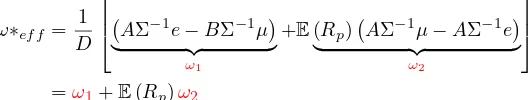
The weights for the efficient portfolio satisfy the the following equation,
ω∗ef f =
1
D
AΣ−1e−BΣ−1µ
| {z }
ω1
+E(Rp) AΣ−1µ−AΣ−1e
| {z }
ω2
[image:16.595.165.431.673.723.2]Which yields,
ω1= 5.316∗10−3
8.77 0.57 0.25 1.36 3.16 0.57 6.59 1.72 2.57 0.47 0.25 1.72 6.04 3.55 1.70 1.36 2.57 3.55 11.63 0.88 3.16 0.47 1.70 0.88 4.88
−1
5.316×
1 1 1 1 1
−0.15451×
1.64% 2.78% 0.05% 0.77% 0.96%
(57) and,
ω2=E(Rp) 5.316∗10−3
8.77 0.57 0.25 1.36 3.16 0.57 6.59 1.72 2.57 0.47 0.25 1.72 6.04 3.55 1.70 1.36 2.57 3.55 11.63 0.88 3.16 0.47 1.70 0.88 4.88
−1
394.79×
1 1 1 1 1
−0.154×
1.64% 2.78% 0.05% 0.77% 0.96%
(58) Hence the efficient frontier can be mapped as follows
ω∗
ef f =
0.08187 (0.21544)
0.66051 0.10715 0.36592
+E(Rp)
4.5709 36.2866 (32.9226)
(4.2105) (3.7244)
(59)
From the efficient set we derive the portfolio variance,
σp2= 1
32.7419 Cµ
2
p−2Bµp+A= 394.7973×µ2p−2×5.3160 + 0.1545
(60)
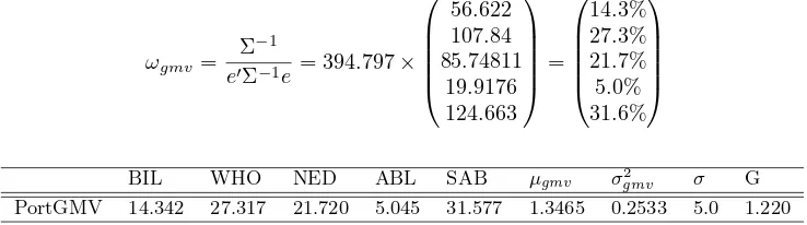
BIL WBO NED ABL SAB E[R] V[R] S[R] Growth
[image:17.595.72.525.90.356.2]Portfolio1 8.2 -21.5 66.1 10.7 36.6 0.0 0.5 6.9 -0.2 Portfolio2 10.5 -3.4 49.6 8.6 34.7 0.5 0.3 5.8 0.3 Portfolio3 12.8 14.7 33.1 6.5 32.9 1.0 0.3 5.2 0.9 Portfolio4 15.0 32.9 16.7 4.4 31.0 1.5 0.3 5.1 1.4 Portfolio5 17.3 51.0 0.2 2.3 29.1 2.0 0.3 5.5 1.8 Portfolio6 19.6 69.2 -16.3 0.2 27.3 2.5 0.4 6.4 2.3 Portfolio7 21.9 87.3 -32.7 -1.9 25.4 3.0 0.6 7.6 2.7 Portfolio8 24.2 105.5 -49.2 -4.0 23.6 3.5 0.8 9.0 3.1 Portfolio9 26.5 123.6 -65.6 -6.1 21.7 4.0 1.1 10.5 3.4 Portfolio10 28.8 141.7 -82.1 -8.2 19.8 4.5 1.5 12.1 3.8
Table 3: A Combination of 20 Portfolios
By varying the portfolio desired return E(Rp), we can trace out the efficient frontier and this is
depicted by the continuous line in figure 1. This demonstrates the diversification benefit of the growth portfolio and the mean variance optimization.
The notable properties of the efficient set is that there exist a portfolio on the frontier which has the minimum variance known as the global minimum variance portfolio and the mean, variance and standard deviation are as follows;
µgmv=
µ′Σ−1e
e′Σ−1e =
5.316045
394.79733 = 1.3465 (61)
σ2
gmv=
1
e′Σ−1e =
1
394.7973 = 0.2533 (62)
Ϯ͘ϬϬй ϯ͘ϬϬй ϰ͘ϬϬй ϱ͘ϬϬй ϲ͘ϬϬй ϲ͘ϬϬй ϴ͘ϬϬй ϭϬ͘ϬϬй ϭϮ͘ϬϬй ϭϰ͘ϬϬй ĨĨŝĐŝĞŶƚ&ƌŽŶƚŝĞƌ w w w G= 'µ−0.5'Σ
>ŽŐŽƉƚŝŵĂůƉŽƌƚĨŽůŝŽ ' ʅ Ϭ͘ϬϬй ϭ͘ϬϬй Ϯ͘ϬϬй
Ϭй ϱй ϭϬй ϭϱй ϮϬй Ϯϱй ϯϬй ϯϱй ϰϬй ϰϱй Ϭ͘ϬϬй
Ϯ͘ϬϬй ϰ͘ϬϬй
Ds Ds& KZW 'KW >K'W
'ůŽďĂůŵŝŶŝŵƵŵ ǀĂƌŝĂŶĐĞƉŽƌƚĨŽůŝŽ ʍ e e e w 1 1 '− − Σ Σ = e e' 1
[image:18.595.187.405.80.228.2]1 − Σ e e e 1 1 ' ' − − Σ Σ µ
Figure 1: Feasible Region MVO and LOGP
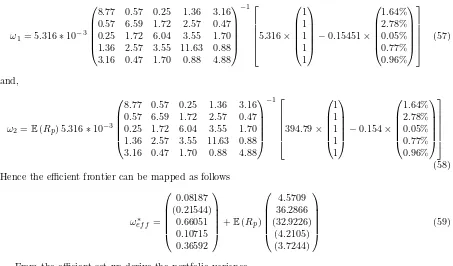
The portfolio weights for the global minimum variance portfolio is therefore;
ωgmv =
Σ−1
e′Σ−1e = 394.797×
56.622 107.84 85.74811
19.9176 124.663
=
14.3% 27.3% 21.7% 5.0% 31.6%
(64)
BIL WHO NED ABL SAB µgmv σgmv2 σ G
PortGMV 14.342 27.317 21.720 5.045 31.577 1.3465 0.2533 5.0 1.220
Table 4: Global minimum Variance Portfolio
4.1.1 LOG-Optimal Portfolio
In case of the log optimal portfolio we can represent the the path followed by each asset as follows,
dS1
S1 = 0.016dt+ 0.094dw1
dS2
S2 = 0.028dt+ 0.081dw2
dS3
S3 = 0.0005dt+ 0.078dw3
dS4
S4 = 0.008dt+ 0.108dw4
dS5
S5 = 0.010dt+ 0.07dw5
(65)
Assuming that the assets are correlated through the wiener term, then the solution to equation [36] is exactly equal to the solution of equation [42]. The feasible region of the growth optimal portfolio and mean variance portfolio
4.2
Calculations2:Efficient Portfolios with a Riskless Asset
With the inclusion of a risky asset and usingµf = 2%
(µ−eµf) =
1.64 2.78 0.05 0.77 0.96
−2.00%
1 1 1 1 1 =
−0.004 0.008
−0.020
−0.012
−0.010
[image:18.595.112.481.295.398.2]Σ−1(µ−eµf) =
0.0088 0.0006 0.0003 0.0014 0.0032 0.0006 0.0066 0.0017 0.0026 0.0005 0.0003 0.0017 0.0060 0.0035 0.0017 0.0014 0.0026 0.0035 0.0116 0.0009 0.0032 0.0005 0.0017 0.0009 0.0049
−1
−0.004 0.008
−0.020
−0.012
−0.010
=
0.0091 2.3046
−3.2907
−0.4793
−1.1235
(67)
H=Cµ2f−2×µf+A= 394.7973×2.002−2×0.15451×2.00 + 5.3160 (68)
= 9.9792 (69)
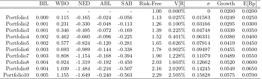
(70) The portfolio weights given a desired level of portfolio return E(Rp)
ω∗=
0.0091 2.3046
−3.2907
−0.4793
−1.1235
×E(Rp)H−2.00 (71)
The optimal portfolio mean,
ω′µ+ (1−ω′e)µf =
0.0091 2.3046
−3.2907
−0.4793
−1.1235
1.64 2.78 0.05 0.77 0.96
= 0.1198 (72)
and the optimal portfolio variance,
ω′Σ−1ω=
0.0091 2.3046
−3.2907
−0.4793
−1.1235
′
0.0088 0.0006 0.0003 0.0014 0.0032 0.0006 0.0066 0.0017 0.0026 0.0005 0.0003 0.0017 0.0060 0.0035 0.0017 0.0014 0.0026 0.0035 0.0116 0.0009 0.0032 0.0005 0.0017 0.0009 0.0049
−1
0.0091 2.3046
−3.2907
−0.4793
−1.1235
= 9.98% (73)
A mapping of different portfolios is therefore tabulated below in table 5 and the graphical representation is shown in
BIL WBO NED ABL SAB Risk-Free V[R] σ Growth E[Rp]
[image:19.595.74.521.536.672.2]- - - - 1.00 0.000% 0 0.0200 0.0200 Portfolio1 0.000 0.115 -0.165 -0.024 -0.056 1.13 0.025% 0.01583 0.0249 0.0250 Portfolio2 0.001 0.231 -0.330 -0.048 -0.113 1.26 0.100% 0.03166 0.0295 0.0300 Portfolio3 0.001 0.346 -0.495 -0.072 -0.169 1.39 0.225% 0.04748 0.0339 0.0350 Portfolio4 0.002 0.462 -0.660 -0.096 -0.225 1.52 0.401% 0.06331 0.0380 0.0400 Portfolio5 0.002 0.577 -0.824 -0.120 -0.281 1.65 0.626% 0.07914 0.0419 0.0450 Portfolio6 0.003 0.693 -0.989 -0.144 -0.338 1.78 0.902% 0.09497 0.0455 0.0500 Portfolio7 0.003 0.808 -1.154 -0.168 -0.394 1.90 1.228% 0.11079 0.0489 0.0550 Portfolio8 0.004 0.924 -1.319 -0.192 -0.450 2.03 1.603% 0.12662 0.0520 0.0600 Portfolio9 0.004 1.039 -1.484 -0.216 -0.507 2.16 2.029% 0.14245 0.0549 0.0650 Portfolio10 0.005 1.155 -1.649 -0.240 -0.563 2.29 2.505% 0.15828 0.0575 0.0700
ϰ͘Ϭй ϱ͘Ϭй ϲ͘Ϭй ϳ͘Ϭй
ϴ͘Ϭй >ŽŐͲŽƉƚŝŵĂůWŽƌƚĨŽůŝŽ
Ő
/>͕ϭ͘ϮϬй tK͕Ϯ͘ϰϱй
E͕ͲϬ͘Ϯϲй >͕Ϭ͘ϭϵй ^͕Ϭ͘ϳϮй
Ͳϭ͘Ϭй Ϭ͘Ϭй ϭ͘Ϭй Ϯ͘Ϭй ϯ͘Ϭй
Ϭй ϭϬй ϮϬй ϯϬй ϰϬй ϱϬй ϲϬй ϳϬй
DŝŶŝŵƵŵ>ŽŐͲsĂƌŝĂŶĐĞ WŽƌƚĨŽůŝŽ
[image:20.595.164.424.86.247.2]ʍ
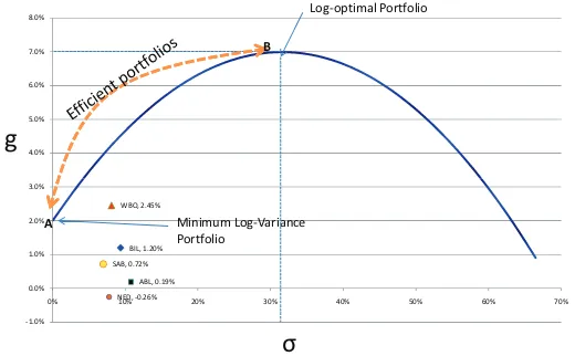
Figure 2: Log Optimal Growth Portfolio
5
Conclusions
In portfolio theory, optimization models play a critical role in determining portfolio investment strategies for investors. Any investment strategy that maximizes portfolio growth has an intuitive appeal for both the professional and non-professional investor. In Markowizt framework one works on diversifying investment assets in order to minimize risk for a given level of return. In this paper we have looked at another portfolio characteristic which is equally important in investment decision process that maximizes the portfolio long term growth rate over a specified time period-the log optimal growth portfolio. We applied our model to five randomly selected JSE stocks. While the Markowizt mean variance strategy is static one period strategy(buy and hold) and a has a fixed time horizon, the log–optimal strategy is dynamic and can be applied to any rebalancing period such as a year, a month a week or a day. The model assumes that stock prices follow a geometric Brownian process and utilizes a stochastic differential equation to quantify the distribution of asset returns. The stochastic process describe the probabilistic evolution of the asset returns through the passage of time. Our model further assumes that asset prices follow a log normal distribution. The solution to the differential equation leads us to conclude that continuously compounded asset return r0,T = T1 ln(SST0) are normally distributed N ∼ (µ−
1 2σ2,σ
2
T ).
This further implies that the future asset priceST is log normally distributed withE(ST) =eµt. This is
a realistic approach to modeling asset prices since a variable that is normally distributed can on negative values something that most financial prices can never do. The distribution of asset returns yields an expected return ofµ−1
2σ2rather thanµhence the log optimal aims at maximizing this geometric mean
representing the long term growth rateG=µ−1
2σ2. There is however a subtle difference between the
two expected value of assets returns7. In our case the portfolio has been formulated in a continuous time framework.If an investor strategy is to maximize long term capital growth then adopting a strategy that maximizes the expected logarithm of returns is considered to be an optimal strategy.
References
Bachelier, L. (1900), ‘The theory of speculation, (published 1900).’,Unpublisedxx, xx.
Benoulli, D. (1954), ‘Exposition of a new theory on the investment of risk.’,Econometrica.22(1), 23–36. Black, F. (1993), ‘Estimating expected return’,Financial Analysts Journal,49, 36–38.
Black, F. & Scholes, M. (1973), ‘The pricing of options and corporate liabilities’, Journal of Political Economy81, 637–659.
Breiman, L. (1961), ‘Optimal gambling systems for favorable games’, Preoceedings of the 4th berkerly Symposium on mathematical Statistics and Probability.1, 65–78.
Campbell, J. Y., Lo, A. W. & MacKinlay, A. C. (1997), The Econometrics of Finanacial Markets, Princenton Univesity Press, United Kingdom.
Christensen, C. M. (2005), ‘On the history of the growth optimal portfolio’,Unpublished.pp. 1–65. Cremers, Jan-Hein, K. M. & Page, S. (2005), ‘Optimal hedge fund allocations: Do higher moments
matter?’,The Journal of Portfolio Management.5, 1–5.
Elton, E. J. & Gruber, M. J. (1974a), ‘On the optimality of some multi-period selection criteria’,Journal of Business47, 231–243.
Elton, E. J. & Gruber, M. J. (1974b), ‘On the maximization of the geometric mean with lognormal return distribution’,Management Science21, 483–488.
Elton, E. J., Gruber, M. J., Brown, S. J. & Goetmann, W. N. (2003), Modern portfolio Theory and Investment Analysis, John Wiley and Sons, New York.
Estrada, J. (2010), ‘Geometric mean maximization:an overlooked portfolio approach’,Unpublished:IESE Business School.pp. 1–31.
Fernholz, R. & Shay, B. (1982), ‘Stochastic portfolio theory and stock market equilibrium’, Journal of Finance27, 615–624.
Hakansson, N. H. (1971), ‘Multiperiod mean-variance analysis: Towards a general theory of portfolio choice’,Journal of Finance.26, 857–884.
Hakansson, N. & Ziemba, W. (1995), Capital Growth Theory:Handbooks in Operations Research and Management Science, Oxford University Press, New York.
Hunt, B. F. (2000), ‘Growth optimal portfolios: their structure and nature’,Unpublished University of Technology Sydney.pp. 1–24.
Hunt, B. F. (2002), ‘Growth optimal investment strategy efficacy: An application on long run australian equity data’,Unpublished:University of Technology Sydney.pp. 1–20.
Hunt, B. F. (2005b), ‘Feasible high growth investment strategy’,Journal of Asset Management. 6, 141– 157.
Kelly, J. (1956), ‘A new interpretation of information rate’,Bell System Techn. Journal 3.35, 917–926. Latane, H. A. (1959), ‘Criteria for choice among risky ventures.’,Journal of Political Economy.52, 75–81. Laten, H. (1959), ‘Criteria for choice among risky ventures’,The Journal of political Economy.38, 145–
55.
Le, T. & Platen, E. (2006), ‘Approximating the growth optimal portfolio with a diversified world stock index’,Journal of Risk Finance.7, 559–574.
Lintner, J. (1965), ‘The valuation of risk assets and selection of risky investments in stock portfolios and capital budgets’,Review of Economics and Statistics.47, 13–37.
Long, J. (1990), ‘The numerarie portfolio’,The Journal of Financial Economics.26, 29–69. Luenberger, D. (1998),Investment Science, Oxford University Press, New York.
Markowitz, H. (1952), ‘Mean-variance analysis in portfolio choice and capital markets’, Journal of Fi-nance.7(1), 77–91.
Markowitz, H. (1976), ‘Investment for the long run:new evidence for an old rule’,Journal of Finance.
XXXI, 1279–86.
Merton, R. (1980), ‘On estimating the expected return on the market’,The Journal financial Economics.
8, 323–361.
Mossin, J. (1966), ‘Equilibrium in capital markets’,Econometrica.35, 768–783.
Norstad, J. (2005), ‘Portfolio optimization unconstrained portfolios’,UnpublishedPart1. Osborne, M. (1959), ‘Brownian motion in stock market’,Operations Research7, 145–73.
Palczewski, A. (2005), ‘Portfolio optimization a practical approach unconstrained portfolios’, Unpub-lished: Institute of applied Mathematics Warsaw UniversityPart1.
Platen, E. (2005), ‘On the role of the growth optimal portfolio in finance.’,Australian Economic Papers.
44, 365–388.
Roll, R. (1973), ‘Evidence on the growth optimum model’,Journal of ScienceXXVIII, 551–566. Samuelson, P. A. (1971), ‘The fallacy of maximizing the geometric mean in long sequences of investing
or gambling’,Procedings National Acad. Sciences USA68, 2493–2496.
Sharpe, W. F. (1964), ‘Capital assets prices:a theory of market equilibrium under conditions’,Journal of Finance.19,, 425–442.
Tim, A. & Kritzman, M. (2007), ‘Mean-variance versus full-scale optimization’, The Journal of Asset Management.7, 1–5.
Tobin, J. (1958), ‘Liquidity preference as behavior towards risk’,Reviewof Economic Studies.25), 65–86. Weide, J., Peterson, D. & Maier, S. (1977), ‘A strategy which maximizes the geometric mean return on
portfolio investments’,Management Science21.
William, J. B. (1936), ‘Speculation and the carryover.’, The Quarterly Journal of Economics.50, 436– 455.
Wilmott, P. (2001),Introduction Quantitative Finance, John Wiley Sons Ltd, New York.
6
Appendix
A
Example
Lets define a simple asset returns asRt= St−St−
1
St−1 whereRt∼N
µ, σ2. Since asset prices are greater
than zero, we haveSt≥0. By implication then:
1 +Rt=
St
St−1 ≥
0, this implies that Rt≥ −1
Then since Rt is assumed to be normally distributed, by symmetry, the probability of Rt ≤ −1 given
thatµ= 0.5 andσ= 0.6 is;
P
R
t−µ
σ
=P(−1.75) = 4.00%