Munich Personal RePEc Archive
Regional disparities and investment-cash
flow sensitivity: Evidence from Chinese
listed firms
Sun, Jianjun and Yamori, Nobuyoshi
Hainan University, Nagoya University
25 April 2009
Online at
https://mpra.ub.uni-muenchen.de/14858/
Regional disparities and investment-cash flow sensitivity:
Evidence from Chinese listed firms
∗Jianjun Sun a and Nobuyoshi Yamori b † a
School of Economics, Hainan University, China
Tel.: +86 898 662 78783; Fax: +86 898 662 81196; E-mail: jianjunsun@hainu.edu.cn
b
Graduate School of Economics, Nagoya University, Japan
Tel.:+81-52-789-4935; Fax: +81-52-789-4924; E-mail: yamori@soec.nagoya-u.ac.jp
Last revised: April 25, 2009
Abstract
In China, regional disparities are important. We examine the difference in the sensitivity of
investment to cash flow between firms in inland regions and those in coastal regions. By using the
financial data of Chinese listed firms, we found that firms in inland regions rely more on their
internal funds in terms of their investment activities than those in coastal regions and that the
sensitivity gap between inland and coastal firms widened in the recent contractionary monetary
policy period. This suggests that firms in inland regions are harder to obtain outside funds due to
unfavorable social and economic environments for inland firms. Our findings suggest that capital
markets in China respond rationally to the potential impact of regional disparities on a firm’s
performance.
JEL Classification O16; G14; G31
Key words: sensitivity of investment to cash flow; sensitivity gap; regional disparities;
Chinese economy
∗
We are grateful to Kei Tomimura and Li Jie for their help. All remaining errors are the responsibility of the
authors. Yamori’s research was financially supported by a Grant-in-Aid for Scientific Research (KAKENHI) from
the Japanese Government.
Regional disparities and investment-cash flow sensitivity:
Evidence from Chinese listed firms
1. Introduction
Listed firms in China are embedded in conspicuous regional disparities.1 In China, the
regional disparities have an impact on the earnings of listed firms through the following three
major channels. First, in the context of a political centralized system, firms in West and central
regions (hereafter, inland regions) carry heavier social burdens than those in the East and coastal
regions (hereafter, coastal regions).2 Second, under the arrangement of fiscal decentralization,
listed firms in inland regions bear directly or indirectly more extra charges than those in coastal
regions.3 Finally, high-quality labor continues to be absorbed by firms in coastal regions and has
boosted these firms to grow more quickly, but the firms in inland regions have been thwarted by
the low level of human capital. Consequently, the three foregoing differences might translate into
performance gaps of a firm, and listed firms in coastal regions tend to perform better than their
inland counterparts.
Based on the above, a reasonable deduction is presented as follows. After a capital market
incorporates the information, firms in inland regions, which have larger uncertainty than those in
1
A long-term unbalanced development strategy (i.e., giving priority to the development of the East and coastal
regions) has resulted in conspicuous regional disparities, (i.e., rich East and coastal regions and poor West and
central regions).
2 For example, there are fewer job opportunities in inland regions, and the State considers employment and social
stability to be important performance measures used by local officials. Therefore, due to the pressure from local
officials who are appointed and dismissed by upper level governments, the listed firms in inland regions have to
hire more redundant workers than those in coastal regions.
3
The reason is that, in comparison to governments in coastal regions, it is difficult for inland governments to
coastal areas, tend to face tighter external financing constraints than those in coastal regions in
terms of their investment decisions. In other words, firms in inland regions might rely more on
their internal funds in their investment decisions than their coastal counterparts. “Unfortunately,
the extant research lacks empirical analyses, which are necessary for addressing the deduction
within the framework of conspicuous regional disparities. We attempt to do this by using the
Chinese stock market and the financial data of listed firms.
A number of studies initialed by Fazzari et al. (1988) argue that firms that face tighter
financing constraints have to rely more on internal funds for making investments.4 However,
Kaplan and Zingales (1997) and Cleary (1999) diverge from these studies by showing that
investment is more sensitive to cash flow for the least financially constrained firms. Allayannis
and Mozumdar (2004) report that Cleary’s findings can be explained by negative cash flow
observations, and Kaplan and Zingales’ results are driven by a few outlying observations in a
small sample. Erickson and Whited (2000) and Alti (2003) argue that the measurement error in
Tobin’s Q affects the estimated investment-cash flow sensitivity. The authors of other recent
papers (Boyle and Guthrie (2003), Moyen (2004), Cleary et al. (2007), and Lyandres (2007))
develop a different theoretical model and offer some explanations for the previously different
empirical findings. In addition, Ağca and Mozumdar (2008) find that there is a decline in
investment-cash flow sensitivity through time and test whether investment-cash flow sensitivity
should decrease with factors that reduce capital market imperfections.
The remainder of the paper is structured as follows. In the next section, we present data and
empirical specifications. In Section 3, we provide the empirical results and discuss their robustness.
4
The last section is the conclusion.
2. Methodology
2.1 Empirical specifications
Following previous studies (Cleary et al. (2007), Lyandres (2007), and Ağca and Mozumdar
(2008)), we use a classical cash flow model to explore the impacts of regional disparities on
investment-cash flow sensitivity. To control for possible heteroskedasticity due to differences in
firm size, we divide both the investment and the cash flow by the net fixed assets (NFA) of the
previous time period. Specifically, the model is as follows.
, 0 1 , 2 , 3 , 1
i t i t i t i t i i t
I
=
α
+
α
CF
+
α
dummyCF
+
α
Q
−+ +
λ
ε
, ⑴Here, Ii, t is defined as the gross investment of firm i for the current year (GIi, t) divided by the
net fixed assets of the previous time period (=GIi, t / NFAi,t-1). CFi,t is the ratio of firm i’s
depreciation plus profits after tax for the current year (DPATi,t) to the net fixed assets of the
previous time period (=DPATi, t / NFAi,t-1). Dummy denotes the regional dummy variable, which
equals 1 if listed firm i locates in coastal regions and 0 otherwise. Therefore, the coefficient of
dummyCF (a cross term of CF and regional dummy) indicates the difference of investment-cash
flow sensitivity between coastal and inland firms. Qt-1 is the lagged one time period Tobin’s Q for
firm i. Due to the measurement difficulty of the marginal Tobin’s Q, empirical studies usually use
the average Q. We follow Kaplan and Zingales (1997), Cleary (1999), and Cleary et al. (2008) and
employ the market-to-book ratio as a proxy for the average Q. Specifically, we calculate the
Chinese Tobin’s Q as follows (Firth et al. (2008)).
Tobin’s Q=(MVCS+BVPS+BVLTD+BVINV+BVCL-BVCA)/BVTA,
firm’s preferred stock, BVLTD is the book value of firm’s long-term debt, BVINV is the book
value of the firm’s inventories, BVCL is the book value of the firm’s current liabilities, BVCA is
the book value of the firm’s current assets, and BVTA is the book value of the firm’s total assets.
Listed firms in China do not issue preferred stocks. Because, until the recent share reform, listed
firms issued both tradable and non-tradable shares, we adjust the measurement of Tobin’s Q.
Specifically, in order to obtain the value of equity in the above formula, we multiply the amount of
tradable shares by the market price and the amount of non-tradable shares by 30% of the market
price (Chen and Xiong (2002) and Firth et al. (2008)).
Based on the fact that ignoring the unobservable factors probably creates an endogenous
problem and a bias in the estimation results, almost all the previous studies in this field (e.g.,
Fazzari et al. (1988), Kaplan and Zingales (1997), Allayannis and Mozumdar (2004), and Ağca
and Mozumdar (2008)) use the firm fixed effects panel regression. We follow them and use the
fixed-effect (demeaned estimation) panel regression.
λ
i andε
i t, refer to an individual firmfixed effect and error term, respectively.
Previous studies (Allen et al. (2005) and Firth et al. (2008)) also suggest that stock returns in
China are less informative of firm performance than those in developed economies because they
tend to reflect market-level information rather than firm-specific information. Consequently,
attention should be given to the potential question of measurement error in Tobin’s Q. Following
Cleary et al. (2008) and Firth et al. (2008), we employ sales growth (SGi,t) as an alternative proxy
of firm performance. Here, SGi,t is defined as the ratio of the difference between firm i’s net sales
in the current year and that in the previous one year to the net sales in the previous one year to
the performance of measure, the model is as follows.
, 0 1 , 2 , 3 , 1
i t i t i t i t i i t
I
=
β
+
β
CF
+
β
dummyCF
+
β
SG
−+ +
γ
μ
,
⑵
2.2 Data and sample description
We use the sample consisting of 1,412 firms that issue only A shares and are listed on the
Shanghai Stock Exchange or the Shenzhen Stock Exchange in China.5 Our data are from the
China Stock Market and the Accounting Research Database (CSMAR). In China, relatively
standardized and internationalized financial regulations were introduced and rigorously enforced
in 1997. Therefore, we construct our data set over the 1998 to 2007 period. To make the sample
more homogenous, the firms in financial industries are eliminated. Firm-year observations are
deleted if the value for net fixed assets or sales is zero or if there are missing values for any of the
five key variables. To avoid distortions arising from mergers and acquisitions, observations with
sales growth exceeding 100% are eliminated (Cleary et al. (2008)). Extreme values of Tobin’s Q
exceeding 20 are also deleted. After that, 9,147 firm-year observations are left. We work with an
unbalanced panel, and our data set covers firms of different sizes and ages from a variety of
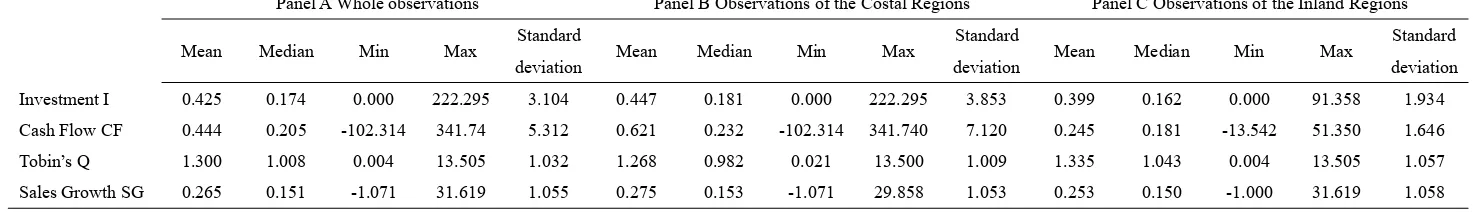
industries. A summary of the statistics of the key variables is presented in Table 1.
Insert Table 1 here.
As is evident from Table 1, the mean investment scaled by the net fixed assets of the overall
sample, the coastal region sub-sample, and the inland region sub-sample are 0.425, 0.447, and
5
A small proportion of the shares of Chinese listed firms are traded at the same time in mainland China, Hong
Kong, and the U.S., and a firm has different stock prices simultaneously inside and outside the mainland because
of capital regulation policies in China. To avoid the measurement question of Tobin’s Q, we exclude these firms. In
addition, because Hainan province and the Guangxi autonomous region have been lagging far behind other coastal
0.399, respectively, which indicates that there is a high investment ratio for Chinese listed firms
and the mean of the investment ratio of firms in coastal regions is slightly higher than that in
inland regions. The sample average cash flow divided by net fixed assets of firms in coastal
regions and in inland regions is 0.621 and 0.245, respectively, which demonstrates that the mean
of the cash flow ratio in coastal firms is much higher than that in inland regions. Based on the
definition of cash flow, this shows that the performance of coastal firms is probably higher than
that of firms in inland regions. From the mean and median of the sales growth rate, firms in both
coastal and inland regions indicated relatively strong growth opportunities during our sample
period.
3. Empirical results
3.1 Tests of regional disparities and investment-cash flow sensitivity
The results of our empirical models based on fixed effects are presented in Table 2. As is
evident form Equation (1) of Table 1, the coefficient on the cash flow is positive and statistically
significant at the 1% level after controlling for investment opportunities. The table shows that
inland firm investment is significantly correlated with proxies for changes in internal funds. The
coefficient of interest is related to the dummyCF (the cross term of regional dummy and cash flow
variables), which allows us to explore whether the regional disparities affect the investment-cash
flow sensitivity of a firm. The coefficient on dummyCF is -0.572 and is statistically significant at
the 1% level, which shows that ①, the coefficient on the cash flow of coastal firms is 0.085, and
their investment is also significantly correlated with cash flow, and ②, there is a significant
sensitivity gap between the inland and the coastal firms. The proxy Tobin’s Q for investment
Equation (1). However, the coefficient on Sales Growth SG, another proxy for investment
opportunities, is negative and insignificant, which indicates, over our sample period, that Tobin’s
Q is probably a better proxy than Sales Growth. The above findings show that the inland firms
rely more on internal funds than those in coastal regions and that inland firms face tighter external
financing constraints than their counterparts in coastal regions.
Insert Table 2 here.
3.2 Time series pattern of the sensitivity of investment to cash flow
Next, we investigate the time series pattern of the sensitivity of investment to cash flow by
running rolling regressions of Equations (1) and (2) for overlapping periods of five years during
our sample period. Our first regression is for the period 1998-2002, the second one, for the period
1999-2003, and so on. We report the results based on the fixed effects model in Table 3. To clearly
view the time series pattern of the sensitivities, we plot the sensitivity of inland firms, the
sensitivity of coastal firms, and the sensitivity gap between the two types of firms. Figure 1
presents the changes of the sensitivities over time.
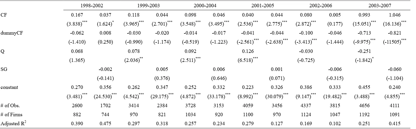
As is evident in Table 3, for six rolling equations of the Q performance, all the coefficients on
CF in six regressions are positive and statistically strongly significant at the 1% level. The results
show that, after controlling for investment opportunities, the internal funds of a Chinese firm in
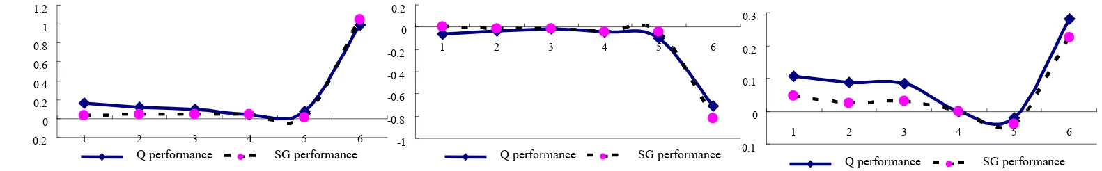
inland regions play an important role in investment decisions. The solid curve in Fig. 1-A depicts
the six coefficients’ time series pattern. The curve indicates that inland firm sensitivity of
investment to cash flow falls slowly for a long time before ascending steeply.
All six coefficients on the dummyCF are negative, which is consistent with our expectations.
financing constraints over the sample period. The first three coefficients are insignificant, but the
last three are significant at the 1% level. The six coefficients on dummyCF, which capture the
sensitivity gap between the inland and coastal firms, are plotted in Fig. 1-B. The solid curve of the
sensitivity gap has two components. The first is nearly a horizontal segment up to the last rolling
period. In this range, the two types of firms maintain a steady sensitivity gap. The second is
steeply downright-sloping, which indicates that, in comparison to coastal firms, firms in inland
regions are forced to rely heavily on internal funds during the last rolling period. The solid curve
of Fig. 1-C tells us that the sensitivity of investment to cash flow in coastal firms depicts the same
time pattern as that in the inland regions in Fig. 1-A. The last sensitivity estimates of inland firms
and coastal firms are 0.993 and 0.280, respectively, which results in a wider difference between
them, reflected by the sharp drop in the gap curve in the figure.
Insert Table 3 here.
Insert Fig. 1 here.
We will now examine the reasons for the results above. Although capital markets in China are
still nascent, they have been growing quickly. During this process of growth, more financial
instruments continued to be introduced, and the informational imperfections in the capital markets
continued being reduced.” This has lowered the external financing constraints and mitigated the
reliance of firms on internal funds. Therefore, the sensitivities of investment to cash flow in both
inland and coastal firms tended to fall gradually, as described by the slowly downright-sloping
segment of the sensitivity curves in Fig. 1-A and C. The result is consistent with that in Ağca and
flow sensitivity decreases with five factors that reduce capital-market imperfections.6
The reasons that the sensitivity curves in Fig. 1-A and C rise steeply during the last rolling
period are as follows. To suppress speculative activities in the real estate market since 2004,
China’s central bank (PBOC) raised the required reserve deposit ratio 14 times from 7% in April
2004 to 14.5% in December 2007.7 The banking sector, which has undergone management
reforms pursuing a value-maximizing target, has to make it difficult for both inland and coastal
firms to obtain external loans.8 In addition, the Chinese financial system has been dominated by a
large state-own banking sector (Allen et al. (2008)), and there is significant reliance on bank loan
finance by Chinese listed firms (Firth et al. (2008)). Hence, we observe a recent steeply rising
segment in the sensitivity curves in Fig. 1-A and C.
Figure 1-B captures the sensitivity gap between both coastal and inland firms. After capital
markets acquire the information that the performance of firms in coastal regions is probably better
than that of those in inland regions, they prefer to offer help to coastal firms that are short of funds
rather than to those in inland regions. The disparity of external financial costs begins to widen. As
compared to firms in coastal regions, firms in inland regions have to rely more on their internal
funds regarding their investment decisions, and, therefore, their sensitivity of investment to cash
6
These five factors are increasing fund flows, institutional ownership, analyst following, antitakeover
amendments, and the existence of bond rating.
7
Specifically, these increases were from 7.0% to 7.5% in April 2004, 7.5% to 9.0% (0.5% every time) in 2006,
and 9.0% to 14.5% (0.5% every time) in 2007.
8
After China’s entry into the WTO in December 2001, the banking sector continued to face increasing pressure
from the competition of foreign financial institutions and to experience many important reforms. In 2005 and 2006,
three of the Big Four banks (BOC, PCBC, and ICBC) successfully partially privatized, accepted investment from
foreign financial organizations, which were subject to the 25% restriction of foreign ownership, and issued IPOs
flow is higher than it is for firms in coastal regions. Interestingly, the sensitivity gap remains
nearly constant until the last rolling sample period. During the last rolling sample of continuously
and strictly contractionary monetary policy, banks experiencing continuous management reforms
have to give priority to allocating scarce credit funds to firms in coastal regions. Although both
types of firms face more external financial constraints over the last rolling period, the
investment-cash flow sensitivity of firms in inland regions rises more quickly than it does for the
coastal firms.
3.3 Robustness tests
Because of the potential question of a measurement error in Tobin’s Q, we substitute another
financial variable (sales growth) for Tobin’s Q as a proxy for investment opportunities. The results
of sales growth measurement are consistent with those of Tobin’s Q measurement. In addition, our
previous results were based on a rolling regression for an overlapping period of five years.
Moreover, when we change the overlapping period (6 years, 7 years and 8 years),9 the previous
results remain unchanged.10 This indicates that our results are robust.
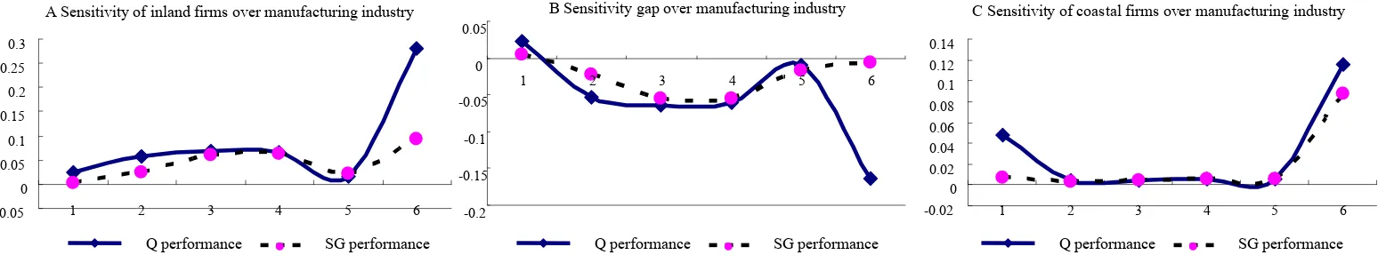
In order to test our findings of robustness further, we choose a typical industry, such as
manufacturing, and use that data from our sample. The empirical results and the time series pattern
of sensitivities are provided in Tables 4 and 5 and Fig. 2.
Insert Table 4 here.
Insert Table 5 here.
9
The definition of sales growth SGt-1 and Equation (2) decide our whole adjusted sample of 8 years, i.e., 2000 to
2007.
10
For space reasons, we do not report the tables for other overlapping periods. These tables are available on
Insert Fig. 2 here.
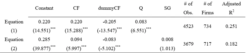
As is evident from Table 4, the investment of both firms in inland and coastal areas is
significantly correlated with their cash flow at the 1% level, and there is still a significant
sensitivity gap at the 1% level. In addition, although the coefficients of Tobin’s Q and sales growth
SG are positive, the former is significant at the 1% level, but the latter is insignificant, which
indicates, for the manufacturing industry, that Tobin’s Q is probably a better proxy for investment
opportunities than sales growth. Figures 2-A and C show the same time series pattern of sensitivity
as that in Fig. 1-A and C. The patterns of the sensitivity gap in Fig. 2-B are not fully consistent, as
a sharp increase of the gap is not found when SG is used. However, as the other results remain
qualitatively unchanged, our findings are robust with regard to the manufacturing industry.
4. Conclusions
To our knowledge, there is no extant research on the impact of conspicuous regional
disparities on investment-cash flow sensitivity. The main goal of our paper is to try to help fill the
gap in the literature by addressing the issue of investment-cash flow sensitivity using Chinese
financial data of listed firms. Our empirical results suggest that firms in inland regions rely more
on their internal funds in their investment activities than those in coastal regions and that the
sensitivity gap between inland firms and coastal firms becomes wider under contractionary
monetary policy. This suggests that regional disparities have a statistically significant impact on
investment-cash flow sensitivity and that it is more difficult for firms in inland regions to obtain
outside funds, such as those from capital markets. Our findings indicate that capital markets in
References
Ağca, Ş., Mozumdar, A., 2008. The impact of capital market imperfections on
investment-cash flow sensitivity. Journal of Banking and Finance 32, 207-216.
Aivazian, V., Ge, Y., Qiu, J., 2005. The impact of leverage on firm investment: Canadian
evidence. Journal of Corporate Finance 11, 277-291.
Allayannis, G., Mozumdar, A., 2004. The impact of negative cash flow and influential
observations on investment–cash flow sensitivity estimates. Journal of Banking and Finance 28,
901-930.
Allen, F., Qian, J., Qian, M., 2005. Law, finance, and economic growth in China. Journal of
Financial Economics 77, 57-116.
Allen, F., Qian, J., Qian, M., Zhao, M., 2008. A review of China’s financial system and
initiatives for the future. Working paper, the Wharton School, University of Pennsylvania.
Alti, A., 2003. How sensitive is investment to cash flow when financing is frictionless?
Journal of Finance 58, 707-722.
Boyle, G., Guthrie, G., 2003. Investment, uncertainty, and liquidity. Journal of Finance 58,
2143-2166.
Chen, Z., Xiong, P., 2002. The illiquidity discount in China. Working paper, International
Center for Financial Research, Yale University.
Cleary, S., 1999. The relationship between firm investment and financial status. Journal of
Finance 54, 673-692.
Cleary, S., Povel, P., Raith, M., 2007. The U-shaped investment curve: Theory and evidence.
Erickson, T., Whited, T., 2000. Measurement Error and the Relationship between Investment
and q. Journal of Political Economy 108, 1027-1057.
Fazzari, S., Hubbard, R., Petersen, B., 1988. Financing constraints and corporate investment.
Brookings Papers Economic Activity 1, 141-195.
Firth, M., Chen, L., Wong, S., 2008. Leverage and investment under a state-owned bank
lending environment: Evidence from China. Journal of Corporate Finance, in press.
Kaplan, S., Zingales, L., 1997. Do investment–cash flow sensitivities provide useful
measures of financing constraints? Quarterly Journal of Economics 112, 169-215.
Lyandres, E., 2007. Costly external financing, investment timing, and investment-cash flow
sensitivity. Journal of Corporate Finance 13, 959-980.
Moyen, N., 2004. Investment-cash Flow Sensitivities: Constrained versus Unconstrained
Table 1
Summary statistics
Panel A Whole observations Panel B Observations of the Costal Regions Panel C Observations of the Inland Regions
Mean Median Min Max Standard
deviation Mean Median Min Max
Standard
Table 2
Empirical results for Equations (1) and (2) over the whole sample period
Constant CF dummyCF Q SG # of Obs. # of Firms Adjusted R2 Equation (1) 0.297 (4.277)*** 0.657 (17.070)*** -0.572 (-14.621)*** 0.022
(0.398) 7256 1240 0.279 Equation (2) 0.301 (8.821)*** 0.652 (15.733)*** -0.543 (-12.237)*** -0.028
(-0.850) 5813 1148 0.432 The values reported herein are the estimates obtained from the firm fixed effect models of (1) and (2) over the whole sample period. Investment normalized by the net fixed assets of a previous time period is the dependent variable. The explanatory variables are the cash flow normalized by the net fixed assets of a previous time period, dummyCF, and either Tobin’s Q (in Equation (1)) or Sales growth SG (in Equation (2)).
t-statistics in brackets. ***, **, and *: significance levels at 1%, 5%, and 10%, respectively.
Table 4
Empirical results for Equations (1) and (2) for the manufacturing industry during the whole sample period
Constant CF dummyCF Q SG # of Obs. # of Firms Adjusted R2 Equation (1) 0.220 (14.551)*** 0.220 (15.288)*** -0.205 (-13.547)*** 0.083
(6.551)*** 4523 734 0.251 Equation (2) 0.285 (39.877)*** 0.094 (5.997)*** -0.083 (-5.102)*** 0.008
(1.013) 3679 717 0.182 The values reported herein are the estimates obtained from the firm fixed effect models of (1) and (2) for the manufacturing industry during the whole sample period. Investment normalized by the net fixed assets of a previous time period is the dependent variable. The explanatory variables are the cash flow normalized by the net fixed assets of a previous time period, dummyCF, and either Tobin’s Q (in Equation (1)) or Sales growth SG (in Equation (2)).
[image:17.595.85.512.481.574.2]Table 3
Empirical results for Equations (1) and (2) over the five-year rolling sample period
1998-2002 1999-2003 2000-2004 2001-2005 2002-2006 2003-2007
CF 0.167 (3.838)*** 0.037 (1.624)* 0.118 (3.965)*** 0.044 (2.701)*** 0.098 (3.548)*** 0.046 (3.495)*** 0.040 (2.536)*** 0.044 (2.775)*** 0.080 (2.872)*** 0.005 (0.177) 0.993 (15.051)*** 1.046 (16.136)*** dummyCF -0.062 (-1.410) 0.008 (0.250) -0.030 (-0.990) -0.020 (-1.174) -0.014 (-0.519) -0.017 (-1.223) -0.041 (-2.561)*** -0.044 (-2.638)*** -0.100 (-3.413)*** -0.046 (-1.444) -0.713 (-9.975)*** -0.821 (-11505)*** Q 0.068 (1.365) 0.078 (2.036)** 0.092 (2.511)*** 0.126 (6.518)*** -0.030 (-0.725) -0.251 (-1.842)* SG -0.002 (-0.141) 0.005 (0.376) 0.006 (0.646) 0.001 (0.071) -0.006 (-0.315) -0.060 (-1.104) constant 0.270 (3.481)*** 0.356 (24.530)*** 0.262 (4.542)*** 0.347 (29.175)*** 0.252 (4.872)*** 0.332 (33.178)*** 0.223 (8.992)*** 0.326 (30.079)*** 0.386 (9.147)*** 0.333 (19.482)*** 0.455 (3.488)*** 0.240 (4.855)*** # of Obs. 2600 1702 3414 2384 3728 3153 4059 3456 4337 3815 4656 4111 # of Firms 882 744 970 821 1034 920 1100 970 1124 1047 1192 1091 Adjusted R2 0.390 0.475 0.297 0.318 0.257 0.234 0.279 0.127 0.169 0.102 0.251 0.415
The values reported herein are the estimates obtained from the firm fixed effect models of (1) and (2) over the five-year rolling sample period. Investment normalized by the net fixed assets of a previous time period is the dependent variable. The explanatory variables are the cash flow normalized by the net fixed assets of a previous time period, dummyCF, and either Tobin’s Q (in Equation (1)) or Sales growth SG (in Equation (2)).
A Sensitivity of inland firms over the entire sample
-0.2 0 0.2 0.4 0.6 0.8 1 1.2
1 2 3 4 5 6
B Sensitivity gap over the entire sample
-1 -0.8 -0.6 -0.4 -0.2 0 0.2
1 2 3 4 5 6
Q performance SG performance
C Sensitivity of coastal firms over the entire sample
-0.1 0 0.1 0.2 0.3
1 2 3 4 5 6
Q performance SG performance
[image:19.842.28.819.182.305.2]Q performance SG performance
Fig. 1 Time series pattern of the sensitivity of investment-cash flow for the entire sample
C Sensitivity of coastal firms over manufacturing industry
-0.02 0 0.02 0.04 0.06 0.08 0.1 0.12 0.14
1 2 3 4 5 6
Q performance SG performance A Sensitivity of inland firms over manufacturing industry
-0.05 0 0.05 0.1 0.15 0.2 0.25 0.3
1 2 3 4 5 6
Q performance SG performance
B Sensitivity gap over manufacturing industry
5 5
1 2 3 4 5 6
-0.2 -0.1
-0.1 -0.0
0 0.05
[image:20.842.30.804.162.319.2]SG performance Q performance
Fig. 2 Time series pattern of the sensitivity of investment-cash flow for the manufacturing industry
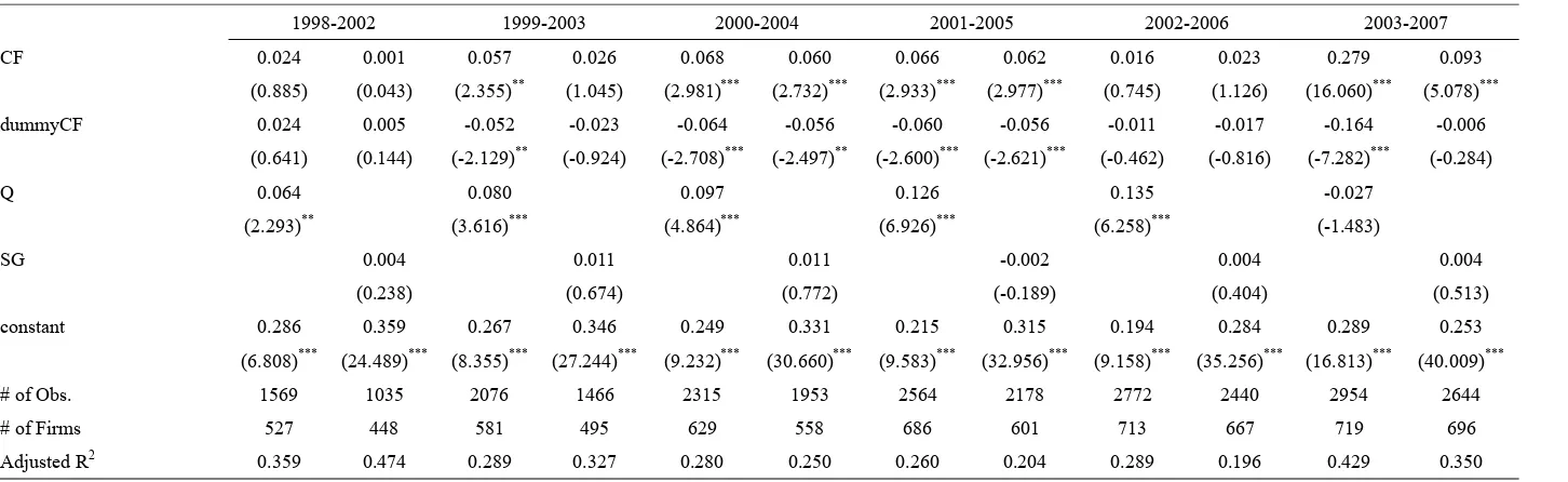
Table 5
Empirical results for Equations (1) and (2) for the manufacturing industry during the five-year rolling sample period
1998-2002 1999-2003 2000-2004 2001-2005 2002-2006 2003-2007
CF 0.024 (0.885) 0.001 (0.043) 0.057 (2.355)** 0.026 (1.045) 0.068 (2.981)*** 0.060 (2.732)*** 0.066 (2.933)*** 0.062 (2.977)*** 0.016 (0.745) 0.023 (1.126) 0.279 (16.060)*** 0.093 (5.078)*** dummyCF 0.024 (0.641) 0.005 (0.144) -0.052 (-2.129)** -0.023 (-0.924) -0.064 (-2.708)*** -0.056 (-2.497)** -0.060 (-2.600)*** -0.056 (-2.621)*** -0.011 (-0.462) -0.017 (-0.816) -0.164 (-7.282)*** -0.006 (-0.284) Q 0.064 (2.293)** 0.080 (3.616)*** 0.097 (4.864)*** 0.126 (6.926)*** 0.135 (6.258)*** -0.027 (-1.483) SG 0.004 (0.238) 0.011 (0.674) 0.011 (0.772) -0.002 (-0.189) 0.004 (0.404) 0.004 (0.513) constant 0.286 (6.808)*** 0.359 (24.489)*** 0.267 (8.355)*** 0.346 (27.244)*** 0.249 (9.232)*** 0.331 (30.660)*** 0.215 (9.583)*** 0.315 (32.956)*** 0.194 (9.158)*** 0.284 (35.256)*** 0.289 (16.813)*** 0.253 (40.009)*** # of Obs. 1569 1035 2076 1466 2315 1953 2564 2178 2772 2440 2954 2644 # of Firms 527 448 581 495 629 558 686 601 713 667 719 696 Adjusted R2 0.359 0.474 0.289 0.327 0.280 0.250 0.260 0.204 0.289 0.196 0.429 0.350
The values reported herein are the estimates obtained from the firm fixed effect models of (1) and (2) for the manufacturing industry during the five-year rolling sample period. Investment normalized by the net fixed assets of a previous time period is the dependent variable. The explanatory variables are the cash flow normalized by the net fixed assets of a previous time period, dummyCF, and either Tobin’s Q (in Equation (1)) or Sales growth SG (in Equation (2)).