Growth, Fiscal Policy and the Informal Sector in a Small Open Economy

Munich Personal RePEc Archive

Growth, Fiscal Policy and the Informal

Sector in a Small Open Economy

Pedro, de Mendonça

Centre for Complexity Science, University of Warwick

5 February 2009

Online at

https://mpra.ub.uni-muenchen.de/13493/

Growth, Fiscal Policy and the Informal Sector in a Small Open

Economy

Gui Pedro de Mendonça

1,2

Abstract: We discuss the implications of informality on growth and fiscal

policy by considering an informal sector based on low tech firms, in an open

economy model of endogenous growth, where labour supply is elastic and

increasing returns arise from public spending. We allow for both labour and

capital to allocate between sectors and examine the dynamic and policy

issues that arise in an economy, where long run outcomes are still dominated

by formal activities, but long macroeconomic transitions arise as a result of

informal microeconomic activities, which take advantage of both government

taxation and limited fiscalization.

International Conference- The Macroeconomic and Policy Implications of Underground

Economy and Tax Evasion, February 5 and 6, 2009 at Bocconi University, Milan, Italy

JEL Classification: C61; E62; F43; O17; O41

Keywords: Endogenous Growth Theory; Optimal Fiscal Policy; Informal Sector; Public Capital.

1_{This research paper was based on one of the chapters from my Master’s dissertation in Economics at} the School of Economics and Management (ISEG), Technical University of Lisbon (UTL), under the supervision of Professor Miguel St. Aubyn (ISEG/UTL). This proposal was devised while waiting for a final decision on my dissertation and benefited from both insightful comments and suggestions by Miguel St. Aubyn. Miguel St. Aubyn is a researcher at the Research Unity on Complexity and Economics (UECE/ISEG/UTL). Original draft from March 2008, this revised version prepared for presentation at the above mentioned conference.

1. Introduction

Ever since the introduction of endogenous growth theory and the increasing returns hypothesis, in the notable Romer (1986) article, theoretical growth economics has debated on the sources of increasing returns and the policy implications of endogenous growth. Earlier contributions by Lucas (1990), Barro (1990), Rebelo (1991), Barro and Sala-i-Martin (1992), Saint-Paul (1992) and Jones, Manuelli and Rossi (1993), suggested that government spending and taxing policies should have an important role on long run growth outcomes. We follow closely this set of proposals and develop a multiple instruments fiscal policy model, based on the Turnovsky (1999) proposal, of an open economy model with an elastic labour supply, where increasing returns arise from productive public spending, to discuss the implications of informality in the outcomes of long run growth and government fiscal policy.

Other recent extensions on the subject of government policy and endogenous growth, which follow similar modelling assumptions as ours, include fiscal policy models, where government spending is used, not only to provide public services, but also to invest in human capital formation, such as Ortigueira (1998) and Agénor (2005). Park and Philippopoulos (2003) discuss optimal fiscal policy and dynamic determinacy in a continuous deterministic endogenous growth model with increasing returns, generated by public infrastructure and additional non productive public spending, specifically public consumption services and redistributive transfers. Still, there is a large scope for discussing policy implications in endogenous growth theory. Our proposal serves this purpose by extending fiscal policy implications when tradeoffs arise from informality, in both capital and labour markets.

The work of Jones and Manuelli (1990) on convex models of endogenous growth provided a framework for introducing long transitions in endogenous growth models. Their proposal consisted in assuming that production was given separately, by two economic sectors with different production technologies, during transitions to the long run. One of the sectors produced macro outcomes with increasing returns, while the other followed neoclassical assumptions. The dynamic outcome of the original hypothesis consisted on a long run growth equilibrium determined by the increasing returns sector and saddle path transitions influenced by the neoclassical sector dynamical decay. Despite providing a simple framework for tackling both, two sector models of endogenous growth and introducing transitional dynamics, this proposal was somehow undermined by the long, rigid transitions arising both from convergence and comparative dynamic analysis. Industrial change and structural adjustment was not as persistent and long as this proposal suggested and, therefore, the Jones and Manuelli (1990) framework was dismissed as a reasonable approach to tackle these

issues. Still, the potential to tackle persistent low tech industrial phenomena, subject to long adjustment periods was there and matched the observed outcomes of informality in developed countries. In Mendonça (2007) 3_{, we propose that the formal vs. informal outcomes for growth}

in a developed open economy may be portrayed in the Jones and Manuelli (1990) fashion. This hypothesis departs from some specific micro and macro assumptions. First, opportunities arise for entrepreneurial informal activities at the micro level, due to government lack of regulation and fiscalization, which can be shown to be consistent with long transitions at the macro level. Second, if we consider the informal sector of the economy to be accountable for long transitions towards long run growth optimal equilibrium, then matching continuous persistence of low tech informal activities can be shown to arise when innovations are considered during transitions. In this framework, informal activities would persist in a sub-optimal continuous adjustment process, where long run outcomes are not be given by a stable steady-state equilibrium, but are a sum of short to medium run periods of transitions.

2. Overview

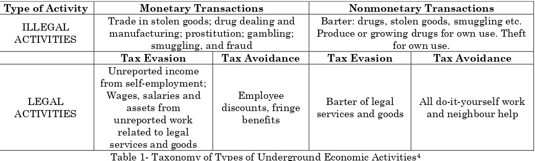
Why is informality both important for growth and policy even in developed countries? Although, this is a current and important topic of development economics research, it has not been considered as a relevant topic in growth theory. This paradigm is based on a stylized fact, which considers that only the large dominant informal sectors of developing countries can be accounted to have both growth and policy implications. Where, in industrialized economies the relevance of this activity is limited and thus negligible. This stylized assumption may have been true for some advanced economies during the post war period, but is certainly not true nowadays. We start defying this assumption by reproducing bellow a table that briefly summarizes informal activities into straightforward categories:

Type of Activity Monetary Transactions Nonmonetary Transactions ILLEGAL

ACTIVITIES

Trade in stolen goods; drug dealing and manufacturing; prostitution; gambling;

smuggling, and fraud

Barter: drugs, stolen goods, smuggling etc. Produce or growing drugs for own use. Theft

for own use.

Tax Evasion Tax Avoidance Tax Evasion Tax Avoidance

LEGAL ACTIVITIES

Unreported income from self-employment;

Wages, salaries and assets from unreported work

related to legal services and goods

Employee discounts, fringe

benefits

Barter of legal services and goods

[image:4.595.38.561.553.711.2]

All do-it-yourself work and neighbour help

Table 1- Taxonomy of Types of Underground Economic Activities4

3_{The basic framework for this model was first introduced in one of the chapters from master} dissertation at ISEG/UTL. This paper extends both the analytical and numerical proposals for the specific case without investment adjustment costs.

4_{Reproduced from Schneider and Enste (2000).}

From all definitions portrayed in table 1, there exists one important characteristic, which is common between all these specific classifications for informality. Each one of us, residents of industrialized countries, has already been, at least, partially exposed to these shadow activities and was given descriptions of these schemes, through third party information, ranging from informal talks to mass media coverage of this phenomenon. The straightforward conclusion for this widespread individual exposition to information on these activities is that they are relevant, persistent and widespread in social economic systems. The differences in both economic scale and diversity of these categories are also evidence that opportunities for profiteering from informality are diverse and not restricted to specific social and economic conditions. They are in fact an emergent macro outcome of social economic systems, arising from agent’s behaviour and microeconomic market conditions. One straightforward conclusion to be drawn is that underground activities, which exhibit characteristics such as persistency, scale and diversity, must have both implications for growth and policy, even in developed economies.

The second hypothesis supporting the stylized assumptions about the implications of informality in industrialized nations, consists on the perceived correlation between informal business scale and economic relevance. The paradigm suggests that if the informal sector is small, then its impact must also be small, even if it persists in the long run. Research on the size and causes of informality contradicts this view for industrialized economies and provides evidence that this phenomenon is not only persistent in developed economies, but has also increased in dimension, during the past two decades, when compared to the relative formal sector dimension on total output share. Schneider (2005) reports an average size for the informal sector relative to GDP of 13,2% in 21 OECD economies, for the years 1989/90, using the currency demand and DYMIMIC method5_{. These values increase to an average size of}

16,4% for the years 2002/03, representing an increase on total output share of about 24% for informal activities, during this recent thirteen years time frame, which represents an average annual growth of about 1,6% for the output share of informal activities. If we extend our time frame some decades to the past, using Frey and Schneider (2001) results, we can emphasize the increasing role of informality in developed economies. They report that Nordic economies, except for Finland, had an average informal sector size of less than 5% relative to GNP in 1960, according to the currency demand method. This output share increases to values of about 15% to 20%, when we consider the year 1995. The growth of output share for informal activities in industrialized economies varies according to the countries we consider, but we can

5_{Dynamic multiple-indicators multiple-causes method. Refer to Schneider (2005) for further details in} this recent modelling technique.

state, with some degree of confidence, that an increasing share of output has been located in the informal sectors of industrialized economies during the past two decades. Moreover, we can also state that this specific sector is no longer residual and in some cases, as in south European countries, it represents between one fifth to almost one third of total output share. What are the causes for this clear trend in developed economies and what are the consequences of this increasing output share for policy outcomes? There are two key causes that may explain this evidence and at the same time are able to capture this trend, even if we consider the specific socio-cultural and political backgrounds of different developed economies. These causes are increasing government spending and bureaucracy, in industrialized countries, during the past four decades. Both these causes are widely accepted for explaining this trend, because they match basic industrial economics theory. Increasing bureaucracy and taxes augment both fixed and marginal costs, distort market prices, consequently, creating legal and economic barriers to entry in the formal sector, decreasing present and future profits for formal sector firms and widening the range of opportunities for illegal activities. We try to tackle these two issues in an endogenous framework for a small developed economy, where informal activities arise during transitions, taking advantage of these arbitrage conditions at the micro level. Peñalosa and Turnovsky (2004) explore these same sources of opportunities for informal activities in a developing economy, considering a CES production function and increasing returns arising from the usual aggregate capital hypothesis. Although, our framework has many similarities with the hypotheses proposed in Peñalosa and Turnovsky (2004), the main scope of their article are the second optimal policies that arise in the presence of a government that lacks revenues and only has access to a limited formal sector for taxation. Other examples of articles that follow similar hypotheses for developing economies in an endogenous growth framework are Braun and Loayza (1994) and Sarte (1999), which tackle the issue of rent-seeking bureaucracies acting through excessive regulation and taxation. Amaral and Quentin (2006) tackle informality in a neoclassical competitive growth framework, where informal managers exchange physical capital for low-skilled labour, in order to cope with limited access to outside investment and financing. The consequences of a growing informal sector are thus evident for both macroeconomic and microeconomic government policy and embody a loss of effectiveness by public authorities to enforce their policies, when facing competition from a sector that acts as a substitute to government regulation, in order to be competitive in a market framework.

background on the Turnovsky (1999) modelling proposal of endogenous growth in small open economy fiscal policy model, refer to Turnovsky (1996a, 1996b). For a detailed overview on the specific dynamics arising in endogenous growth models of open economies, following this basic framework, refer to Turnovsky (2002). For a complete overview and additional proposals on this class of models, considering both an elastic labour supply and adjustment costs, refer to Mendonça (2007).

3. The Model

6

This economy will consist of

N

identical households and firms. Aggregate conditions are given by equation (A1) and households can allocate their time between labour,

(

, and leisure, l, which are set endogenously by model dynamics.

)

1−l

1

,

,

1,2

n

i i i

i

X

x N

X

X

i

=

=

=

∑

=

(A1)

The representative agent’s welfare is given by the following intertemporal isoelastic utility function, as in Turnovsky (1999). Equations (A2) and (A3) define the individual’s utility and the aggregate utility for this economy, respectively:

( )

0

1

t

U

cl

θ γ

e

ρ

γ

∞ ₋

=

_∫

dt

(A2)

(

)

0

1

/

t

U

C

N l

θ γ

e

ρ

γ

∞ ₋

⎡

⎤

=

_∫

_⎢

_⎣

_⎥

_⎦

dt

γθ

(A3)

(

)

0 ; - 1 ; 1 1 ; 1

θ> ∞ < <γ >γ +θ >

As usual C stands for aggregate private consumption, c is the household consumption, and parameters and , are related with the intertemporal elasticity of substitution and the impact of leisure on the utility of the representative agent, respectively. The constraints imposed on the parameters are necessary to ensure that the utility function is concave in c

and l.

γ θ

In this economy positive externalities are the result of public productive capital. Output for the individual formal firm is determined by a Samuelson type production function with non-excludable and non-rival public goods. Our proposal follows closely the well known hypotheses defined in Barro (1990) and Barro and Sala-I-Martin (1992). The formulation followed here is a variation to assume an elastic labour supply, as described in Turnovsky (1999):

6_{For reasons of simplification, we discard the use of the time subscript in the time varying variables of} our model. The meaningful variables are consumption, investment, domestic capital accumulation and foreign debt accumulation. Leisure, labour allocation and government spending are given endogenously and are also subject to transitions.

(

)

1

1 1 1

y =AGβ ⎡_⎢⎣ −l ⎤_⎥⎦φk₁ −β (A4)

(

) (

)

1 / 1 1 1

y =A G k β _⎣⎢⎡ −l ⎤_⎥⎦φk₁ (A5)

1

0

1

G

=

gY

< <

g

(A6)

( )

(

)

1

1 ₁

1 1 1 1

Y K A gN l K

φ

β −β _−β

⎛ _{⎡ ⎤ ⎟}⎞ _{⎡ ⎤} ⎜

=_{⎜⎝ ⎢⎣ ⎥⎦ ⎟⎟⎠ ⎢⎣} − _{⎥⎦ 1}

β

)

1

(A7) 0< <β 1, 0< <φ 1, φ<β, 0< <α 1

Output for the individual formal firm, , is given by the usual neoclassical Cobb-Douglas production function, (A4). The endogenous variable defines the percentage of time devoted to working in the formal sector by our representative agent. This endogenous variable is included to ensure the normalization of the labour input to one is maintained and because it gives a straightforward option for taking an optimal control rule for labour allocation between sectors. As it is our intention to maintain the labour input normalized to one, will vary between zero and one, and labour allocation in the informal sector will be just

1

. As usual in economic growth formalizations, denotes the individual firm capital stock and the aggregate capital stock. G represents aggregate public spending and g the share the government share of formal output. Parameters A, , and φ stand for the formal exogenous technology and the elasticities of government spending and labour, respectively.

1

y

1

β

1

1

−

i

k

K

_i

In order to obtain an AK technology in the aggregate framework it is convenient to tie government expenditure, G, to aggregate formal output, , where g acts as an endogenously determined fraction of government expenditure relative to aggregate output. Applying aggregate conditions to the representative firm production, (A4), we obtain the aggregate formal output for this economy, as expressed in (A7). Parameter restrictions are given above and a restriction to guarantee that labour productivity is diminishing in the aggregate,

, is additionally considered.

1

Y

1

φ< −

The government sector of this economy can only observe and tax activities that occur in the formal sector. We consider, for reasons of simplification, that the public sector must always manage a balanced budget with no possibility of issuing public debt bonds. As public spending has been tied up to aggregate output, it follows that the balanced government budget constraint is given by:

(A8)

(

1

1

(1

)

1 1 1

c

C

w

w

l

N

k k

r K

T

gY K

τ

+

τ

−

+

τ

+ =

Where, , represent taxes on wage income for formal sector labour allocation, , capital income taxes on revenues from entrepreneurial formal activities, , consumption taxes and finally a lump sum tax given by

w

τ

τ

_k

c

τ

T N

τ

=

. Taxes on foreign bonds, , are a possibility considered in Turnovsky (1999) that we relax in our framework. This excludes the possibility of subsidies on foreign debt accumulation, without imposing an additional parameter restriction, and has no relevant implications on the dynamic behaviour of this economy.

b

τ

The representative firm in the informal sector will also have its output given by a Cobb-Douglas production function, following the same structure of (A4), where all productive factor intensities, including the elasticity of the government input, are lower than the ones considered for the formal sector production function. These hypotheses are necessary in order to obtain static equilibrium conditions for capital and labour decisions between sectors. They are also reasonable if we consider that informality arises, in order to take advantage of the absence of government regulation and taxation. Therefore, in spite of using a worst technology, they are still able to participate with success in a competitive market framework. Following this short intuition, the production function for the representative firm in the informal sector comes:

(

)(

)

2 1 1 1

y =DGβ −μ _⎣⎢⎡ − −l ⎤_⎥⎦ξk₂η (A9)

( ) (

)(

)

1

2 1 1 1 1 2

Y =D gY β μ− _⎣⎢⎡ − −l _⎦⎥⎤ξK Nη −η (A10)

(

)

( )

1 ( ) ( )(11 1 ) (1 )

(

) ( )

( 1) (1 )

2 1, 2 1 1 1 1 - 1 2

Y K K D Ag N l Kβ μK

β β μ η β φ β μ φ β μ ξ β

β μ _ξ

η

β β

β β −

− + − − − − + −

−

− −

− −

= − (A11)

0≺ ≺μ 1 , β μ , 0≺ ≺ξ 1 , φ ξ , 0≺ ≺η 1 , 1−β η,A D

Where D, represents the usual exogenous technological infrastructure, which is smaller than the one of the formal sector, A. The elasticities for the capital and labour inputs are different and restricted to be smaller than the ones in the formal sector. Labour allocation by the representative agent is given by expression

(

)

1

1− . Informal sector firms are still able to benefit from public goods and services, but face fiscalization of its use by the authorities, which diminishes the factor intensity for public services to be just, β . Parameter μ can therefore be used to determine the impact of fiscalization by authorities. This specification could be extended to other productive factors, where one could distinguish between factor fiscalization. In this framework, for reasons of simplification, only the dimension described above will be considered.

μ

−

It is straightforward to observe that output in the informal sector will depend on output from the formal sector, due to the capacity of using public capital, though restricted by government fiscalization. As all productive factor intensities of the informal individual firm technology are lower than the ones from firms in the formal sector, investment and labour decisions in this economy will only occur if the net factor payments are equal between the two sectors. These conditions come as follows:

(

)

,

,

1

i

k i i

i

dy

dy

r

w

dk

d

l

=

=

−

i _(A12)

(

1

−

τ

w

)

w

1

=

w

2

,

(

1

−

τ

k

)

r

k₁

=

r

k₂

2

y

(A13) Applying the usual marginal productivity conditions described in (A12) to the equilibrium

conditions described in (A13), we obtain the labour and capital market equilibrium conditions for this economy:

(A14)

(

1−τ φw

)

y1 =ξ

(

)(

)

1

1 2

1

_k

1

y

k

k

τ

β

η

−

−

=

y

2 _(A15)

Solving (A14) for and then substituting it in (A15), we obtain static relation condition for capital between the two sectors:

1

y

(

)

(

)(

)

2 1 1 1

1

,

1

1

w

k

k

k

η

τ φ

τ

β

−

= Θ

Θ =

−

−

ξ

(A16)

Substituting (A8) in equation (A4), output of the representative firm and aggregate production for the informal sector are obtained as follows:

( )

(

)(

)

2 1 1 1 1 1 1

y k =DGβ−μ_⎣⎢⎡ − −l ⎤_⎥⎦ξΘηk η (A17)

( )

(

)(

)

1

2 1 1 1 1 1 1 1

Y K =Dgβ−μ _⎣⎢⎡ − −l ⎤_⎥⎦ξΘηYβ μ− K Nη −η (A18) Substituting in expression (A18) and rearranging the terms, aggregate output for the

informal sector is now given by the model parameters, formal sector aggregate capital and the endogenous variables governed by the model:

1

Y

(A19)

( )

2 1 1 1

Y K

= ΩΘ

D

η

K

β +η−μ

Where parameter Ω is equal to:

( )

₁ ( ) ( )(11 1 ) (1 )

(

) ( )

( ₁) (1 )

1 1 1 1

-Ag N l

β β μ η β φ β μ φ β μ ξ β

β μ _ξ

β β

β β

− + − − − − + −

−

− −

− −

Ω = − (A20)

The following parameter restrictions must now be imposed in order to assure that capital and labour are diminishing in the aggregate:

(

) (

)

1 , 1 1

β + −η μ≺ φ β−μ +ξ −β ≺ −β

)

ξ

(A21) Applying the static market equilibrium conditions necessary for the existence of these two

sectors in a competitive economy, has produced two technologies that depend only on the parameters, exogenous population employed in both sectors and capital employed in the formal sector. This style of formalization provides a clear strategy for modelling an economy, where decisions, such as capital accumulation and investment, are based solely on the formal sector variables. Informal sector capital inputs enter this economy through the static equilibrium condition given by (A16). We will consider that formal aggregate capital employed in production is always bigger than aggregate informal capital. This restriction is consistent with data and research on the informal sector size of developed economies. Recalling the market clearing condition for individual firm capital between sectors, (A16), we will just impose that , in order to guarantee that this empirical evidence is always satisfied.

(

1 _w

)

(

1 _k

)(

1

η −τ φ < −τ −β

Following this strategy of modelling will allow us to develop a two sector continuous time dynamic model, without having to tackle with the difficulties that arise when dealing with a two sector economy maximum problem7_{. Considering a neoclassical production function for}

the informal sector that depends exclusively on formal capital, will also be consistent with the existence of transitional dynamics, since total output for this economy is given separately8_{. We}

will deal with this subject later on, when deriving an analytical solution for the transitions dynamics of this economy, however, this subject can be described intuitively by a simple analysis of the aggregate marginal productivity of capital. Taking a partial derivative of on

, we obtain:

1

Y

1

K

( )

₍

1 1

1 1 '

2, 1 1

K

Y K

Y

Y

K

=

+

'

)

K

K

, it is clear that this expression still depends on formal sector capital, which in turn depends on time.

Considering the usual endogenous growth hypotheses, where capital grows at a constant growth rate, we can obtain a simple asymptotic rule guarantying that long run output will depend only on formal sector activities:

7_{The formalization of the two sector economy optimal control problem is reproduced in the appendix.} 8_{Barro and Sala-i-Martin(1999) discuss both this strategy and the CES production function formulation,} in pages 161 to 167 of their book.

( )

1 1

1 1 '

1

lim

_K k

Y K

Y

K

→∞

=

, this result is consistent to restrictions imposed on parameters on equation

(A19), which imply that the marginal productivity of aggregate informal capital will decline asymptotically, until it becomes negligible on the long run.

Assuming that capital depreciates at the constant rate equal to δ, the representative firm intertemporal capital accumulation constraint is given as usual by:

(A22)

-

,

1,2

i i i

k

=

i

δ

k i

=

In a small open economy framework, it is standard to assume that individuals and firms have full access to international capital markets and can accumulate debt (or foreign bonds) at an exogenously given world interest rate. As a result, the intertemporal budget constraint facing the representative agent in this economy will be equal to individual consumption, c, plus investment, , and debt interest payments, rb, minus capital and labour incomes, and

i

i

r k

_{k i}

(

1

)

i

w −l

2

1

r k

_k

0

0

, assuming that the representative agent is a net borrower9_{. To obtain this specific}

constraint according to the assumptions described in previous chapters, we only need to consider the additional government revenue implications, as defined in equation (A8).

(

1

c

)

1 2

(

1

w

) (

1

1

)

1

(

1

k

)

k₁ 1 2

(

1

)(

1

)

₂

b

=

+

τ

c

+ + +

i

i

rb

+ − −

τ

τ

w

−

l

− −

τ

r k

−

w

−

l

−

−

(A23)

3.1. Dynamic general equilibrium conditions for labour allocation and leisure

Substituting the functional form for the representative agent utility in the optimality conditions, (A70) and (A71), for consumption and leisure, we obtain the representative agents intertemporal conditions for consumption and labour/leisure decisions:

(A24)

(

)

1

1 _c

cγ−lθγ +λ +τ =

(

)

(

)

1

1 1 2 1

1

_w

1

c l

γ θγ

w

w

θ

−

₊

λ

⎡

₋

τ

₊

₋

⎤

₌

⎢

⎥

⎣

⎦

(A25)

(

1

w

) (

w

1

1

l

)

w

2

(

1

l

)

λ

⎡− −

_⎢⎣

τ

− +

−

⎤

_⎥⎦

=

0

(A26) Applying market clearing and aggregate conditions to expressions (A24) and (A25),

substituting then the optimal control for aggregate consumption obtained from (A24), in the macroeconomic labour/leisure condition obtained from (A25), and rearranging in an intuitive form, we obtain the dynamics for labour and leisure in this economy:

9_{This type of intertemporal budget constraints leaves the possibility of analyzing agents and economies} that act as net lenders also.

(

)

(

) ( )

1 1

(

1

)

2

(

1 2

)(

1

)

1

1

1

,

1

c

w

C

l

l

Y K

Y K K

θ

τ

τ φ

ξ

+

=

−

−

+

−

(A27)

(

)

(

(

) ( )

1

)

1 1

1

lim

1

1

c t

w

C

l

l

Y

θ

τ

τ φ

→∞

+

=

−

−

K

(A28)

Following the same strategy for optimal labour allocation, we obtain from (A26), the expressions that determine the dynamics of labour allocation during transitions and in the long run:

(

1−τ φw

) ( )

Y K1 1 =ξY K2

( )

1 (A29)

(

)

(

)(

(

) ( )

)

1 2 1 2

1 1 1 1

1

,

1

_w

Y K K

Y K

ξ

τ φ

−

−

=

−

1

1

(A30) This implies that in the long run

(

)

.

1 1

lim 1

0

lim

1

t→∞

−

= ⇒

t→∞

=

This section introduced the issue of informal entrepreneurial activities that are based on the existence of microeconomic assumptions, which do not hold on the aggregate framework. Recall from equation (A26), the optimality condition for labour allocation, where we obtained the same market clearing condition, (A13), that we have proposed initially for labour allocation. However equations (A29) and (A30) clearly show that at the macro level, long run equilibrium will be defined solely by formal activities and informal activities have their existence limited to transitions to the long run outcome. This concept is also observed in the behaviour of labour/leisure to equilibrium, where the long run equilibrium expression, (A28), follows the optimal condition for this class of utility functions, when and an optimal control problem of endogenous growth with just one state condition is considered.

1

=

1

3.2. Capital market equilibrium assuming no information between sectors

For the moment, we will continue to assume that our optimal control problem is given by the three state conditions described in section 1. of the appendix. The first consequence of this assumption is obtained from the optimality conditions for investment decisions, (A73) and (A74), which state that the shadow prices of foreign and domestic capital must equalize.

(A31)

1 2

q

=

q

= −

λ

Substituting this condition in the co-state conditions, (A76) and (A77), for domestic capital accumulation, we obtain the micro equilibrium condition for domestic capital accumulation that we defined theoretically in (A13). However, as in labour allocation and leisure decisions, this condition does not hold, when the dynamic general equilibrium conditions are considered:

(

)(

) ( )

1 1 2

(

1 2

)

1 2

,

1

_k

1

Y K

Y K K

K

K

τ

β

η

−

−

=

(A32)

Equation (A32) defines a long run equilibrium condition between formal and informal aggregate capital, which is not viable asymptotically, when we consider formal aggregate capital to grow at a constant rate and informal aggregate capital to decay asymptotically after reaching a maximum. In this case, the indifference between accumulating foreign bonds, defined in the Keynes-Ramsey consumption equation (A33), or domestic capital, would reduce to the simpler case with one formal sector of production, where informal activities would only play a role in the aggregate budget equilibrium outcome and no role in consumption decisions.

(

)

(

1

)

r

C

ρ

γ

−

=

−

C

(A33) This assumption is contrary to empirical results on underground activities, which relate the

majority share of its revenues to short and medium run consumption by their holders. This logic is related both to the motivations of agents to participate in these activities and government fiscalization limitations. Most of the participants in this type of activities accept the risk of being caught, in exchange of the possibility to expand their consumption share. On the other hand, fiscalization by authorities reinforce this incentive, due to the obvious limitations to control everyday consumption activities, where it is difficult to assert the origin of this type of revenues, without imposing excessive limitations on commercial transactions.

3.3. Capital market equilibrium assuming asymmetric information in investment decisions

To tackle the problems discussed in the previous two sections, we propose to define possible criterions to obtain an optimal control problem that is consistent with a endogenous growth model with long transitions, following the Jones and Manuelli (1990) proposal. This hypothesis is consistent to consider that the long run is a sum of short and medium run specific periods and that in all of these shorter periods, opportunities for entrepreneurial informal activities arise. As a specification consistent to the Jones and Manuelli (1990) hypothesis produces periods of long transitions to steady-state endogenous growth, it provides an ideal benchmark framework to deal with the issue of informality in a macroeconomic context. First, we know that at the micro level opportunities to engage in informal activities arise from multiple possibilities in developed economies such as excess bureaucracy, unregulated technological innovation 10_{, barriers to entry and our specific proposal of excess}

10_{The Internet history provides a vast set of examples of informal activities that not only took} advantage of existent technology but also introduced innovations, in order to obtain market shares of unregulated activities. In some cases, as the electronic music market, reached the proportions of an industrial phenomenon. In the long run, however, the majority of these operations were driven, by

taxation. Second, we know that in developed economies the formal sector activities are dominant in the long run outcomes of society, which is consistent with the outcome of an endogenous growth model driven by formal sector activities, as our proposal suggests. In order to obtain this outcome, we just need to define a different level of information available to households and firms about the relation between both productive sectors. In this section, we assume that agents have information about the linear relation between capital11_{, (A16), but}

lack information about investment decisions between sectors.

Substituting the relation for capital between sectors, (A16), in the optimization problem described in section 1. of the appendix, we can rewrite both the new representative agent co-state and aggregate conditions for capital accumulation easily:

(A34)

(

)

(

(

)

_{1 2}

1 2 1

1

k k k

q

=

ρ

+ Θ

δ

q

+

λ

−

τ

r

+ Θ

₁

r

)

(

)

(

)(

) ( )

1 1 2

( )

1

1 2 1 1

1 1

1 _k 1 Y K Y K

q q

K K

ρ δ λ⎛⎜⎜ τ β η ⎞⎟⎟

= + Θ + _⎜⎜ − − + Θ _⎟

⎟⎟

⎜⎝ ⎠⎟

(A35)

Where

(

)(

)

(

)

(

)(

)

2 1

1

1

1

1

1

1

k w

k

τ

β ξ

η

τ

τ

β ξ

−

−

+

−

Θ = + Θ =

−

−

φ

.

In this case, we can easily observe that the remaining co-state condition for informal capital has no useful information for our optimal control problem. Therefore, we are still considering a three state optimization problem, which could be reduced to a two state problem had we decided to deal with aggregate capital accumulation instead of specific to sector capital accumulation. The results of this option, however, would produce the same analytical outcome and would not add additional hypothesis to our strategy.

To obtain the aggregate expression that is crucial to guarantee indifference in accumulation between foreign and domestic capital in this economy, we just need to consider the optimal investment condition (A73) and substitute it in the co-state conditions (A75) and (A35). Then, we can either obtain the two possible Keynes-Ramsey rules of consumption or solve the two dimensional endogenous system of co-state variables, to obtain the intertemporal financial rule for indifference in capital accumulation:

(

)(

) ( )

1 1 2

( )

1 1

1 1

1

_k

1

Y K

Y K

r

K

K

τ

β

η

= −

−

+ Θ

− Θ

₂

δ

(A36)

regulation and fiscalization by authorities, and economies of scale from formal sector firms, to adopt legal standards, face closure or reduce their activities to a residual and undetectable dimension.

11_{This assumption will imply that from now on we will consider (A17) to be the individual firm informal} production technology, in substitution of (A9), and informal aggregate output to be defined by (A18) instead of (A11). This assumption is necessary in order to consider just one state condition for capital accumulation and does not alter the dynamic general equilibrium conditions considered in section 3.1..

(

)(

) ( )

1 1 2 1

lim

1

_k

1

t

Y K

r

K

τ

β

→∞

= −

−

− Θ

δ

(A37)

We take the option of not dealing with this hypothesis further and leave just this short introduction to the issue of limited information. This decision is based on the fact that the asymmetric information about investment decisions case is less tractable analytically, than the full information hypothesis of the subsequent sections. In spite of that, the strategy to solve analytically both for the long run and transitional dynamics, will follow closely that from the complete information case, although, much less intuitive. One of the main interests of this hypothesis is discussed in Mendonça (2007), where it is shown that the existence of a set of endogenous rules for the existence of an optimal fiscal policy 12_{, as described in Turnovsky}

(1999), is no longer available and public choice outcomes must arise, when a full information central planner is considered.

3.4. Capital market equilibrium assuming complete information about investment decisions

It is straightforward to obtain a linear relation for investment decisions between sectors using the linear relation for capital, already defined in (A16), and both the capital accumulation differential equations, defined by (A22). Extending the informal sector accumulation condition as a function of formal capital, following (A16), we obtain the following linear endogenous solution for investment decisions.

(

)

(

)(

)

2

1

1

1

w

k

i

η

τ φ

τ

β ξ

−

=

−

−

i

1

(A38) This simplifying assumption is necessary to fully internalize the information about informal

activities, as a function of formal sector variables, and is consistent with the existence of a balanced growth path governing capital accumulation and no non-linear assumptions about investment decisions. Discarding capital accumulation in the informal sector and substituting the linear relation for investment in the households intertemporal open economy budget

β

12_{In our multiple fiscal policy framework with just a formal productive sector, optimal fiscal policy is} defined by a set of endogenous linked fiscal rules that can be defined to be consistent to the neoclassical assumptions on growth maximization, no taxes on productive factors and a government size consistent with its input elasticity ( ), guarantee that the Ramsey (1927) optimal taxation principle is achievable and endogenously given. In our specific choice of households utility, the rule that guarantees a fiscal policy that minimizes the decrement of utility, in order to minimize the economic distortion of taxation (excess burden), not taking into account the equity and redistributive aspects that may arise from fiscal policy, is given by

0

k

g

τ

= ⇒ =

w c

τ

τ

−

=

. This rule defines a framework where taxes on leisure are obtained by subsidizing labour, so that both consumption and leisure, the two utility enhancing activities, are taxed uniformly resulting in a dynamic application of the Ramsey optimal taxation principle. This short description resumes the findings of Turnovsky (1999) for this class of fiscal policy endogenous growth models and builds on its main assumptions.

constraint, our optimal control problem is reduced to a two state optimal control problem with just one optimal control condition for investment decisions.

(A39)

1

q

= − Θ

λ

₂

1

r

(

)

(

)

_{1 2}

1 1

1

k k k

q

=

ρ

+

δ

q

+

λ

⎡

_⎢

−

τ

r

+ Θ

⎤

_⎥

⎣

⎦

(A40)

Applying market clearing and aggregate conditions, we obtain the dynamic general equilibrium co-state condition for formal capital:

(

)

(

)(

) ( )

1 1 2

( )

1

1 1 1

1 1

1 _k 1 Y K Y K

q q

K K

ρ δ λ⎡⎢ τ β η ⎤⎥

= + + _⎢ − − + Θ _⎥

⎢ ⎥

⎣ ⎦

(A41) Substituting the optimal control expression for investment, (A39), in (A41), and then following

the same strategy for obtaining the two possible optimal Keynes-Ramsey consumption rules, we obtain the transitions and long run endogenous expressions for financial equilibrium in this economy:

(

)(

) ( )

1 1 2

( )

1 1

2

1 1

1 _k 1 Y K Y K

r

K K

τ β η

− ⎡⎢ ⎤

= Θ _⎢ − − + Θ −

⎢ ⎥

⎣ 1 ⎦

δ

⎥

⎥ (A42)

(

)(

) ( )

1 1 1

2

1

lim

1

_k

1

t

Y K

r

K

τ

β

−

→∞

= Θ

−

−

−

δ

(A43)

3.5. Long run equilibrium dynamics for the full information economy

Assuming no further hypotheses about non-convexities, the dynamic long run outcome for the complete information economy can be obtained, through solving the simple usual dynamic case of endogenous growth in a small open economy. Substituting the steady state condition, defined by (A42), in the differential equation for consumption, (A33), we obtain the intertemporal Keynes-Ramey consumption rule:

(

)(

) ( )

1 1 2

( )

1 1 2 1 1 1

1

1

1

k

Y K

Y K

K

K

C

C

ρ

δ

τ

β

η

γ

−

⎛

⎡

_{⎤ ⎟}

⎞

⎜

_⎢

_{⎥ ⎟}

⎜

_{+ − Θ}

₋

₋

_{+ Θ}

_⎟

⎜

⎢

⎥ ⎟

⎜

⎟

⎜

⎢

⎥ ⎟

⎜

⎣

⎦

⎟

⎜

⎟

=

_⎜

_⎟

⎟

⎜

−

_⎟

⎜

_⎟

⎜

_⎟

⎜

⎟

⎜

_⎟⎟

⎜⎝

⎠

(A44)

The intertemporal aggregate budget constraint for the decentralized full information economy comes:

(A45)

(

)

(

)(

)

(

)

1 11

( )

21

(

1

)

1 2

( )

1

1

1

1

1

1

c

k w

B

C

I

rB

T

Y K

Y K

τ

τ

β

φ

τ

ξ

η

=

+

+ Θ +

+ −

⎡

⎤

⎡

−

_⎢

_⎣

−

−

+

−

_⎥

_⎦

−

_⎢

_⎣

−

+ Θ

⎤

_⎥⎦

Substituting again the exogenous international interest rate, by the steady state rule of indifference in accumulation, (A42), investment by the capital accumulation equation and rearranging in the usual form, the net wealth differential equation for this economy comes:

(A46)

2 1 2 1

W

= Θ

K

−

B

⇒

W

= Θ

K

−

B

( ) ( )( ) ( )

( )

₍

₍

₎

₎

₍

₎

1 1 1 2 1 1

2 1 1

1 1 2 2

1

1

1

1

1

1

k w dom

dom c

Y K

W

W

K

Y K

W

C

K

τ

β

φ

τ

ω

δ

η

ξ

ω

τ

−

−

⎡

⎤

⎢

_⎡

_⎤

⎥

=

Θ

_⎢

_⎢

_⎣

−

−

+

−

Θ − Θ

_⎥

_⎦

_⎥

+

⎢

⎥

⎣

⎦

⎡

⎤

⎢

⎥

+

_⎢

Θ +

−

Θ

_⎥

Θ

− +

−

⎢

⎥

⎣

⎦

2 2

T

(A47) Where 1

dom K W

ω = .

We have considered the parameter related to aggregate labour incomes, in order to simplify our system. This parameter has no transitions in the long run, when the growth rates of net wealth and formal capital equalize. We will use it to define the long run endogenous equilibrium and discuss the issue of transitions in the following sections.

dom

ω

We can now describe the long run endogenous equilibrium for this economy by applying the standard asymptotic assumptions, about labour allocation, production and leisure, to the system defined by (A44) and (A47). The long run dynamical system is given by:

(

)(

) ( )

1 1 1 2 1 / 1 1 1 k

l r l r

Y K

K C

ρ δ τ β

γ −

⎛ _⎞⎟

⎜ _⎟

⎜ + − Θ − − ⎟

⎜ _⎟ ⎜ ⎟ ⎜ ⎟ ⎜ ⎟ = ⎜_{⎜ − ⎟⎟} ⎟ ⎜ _⎟ ⎜ _⎟ ⎜ _⎟ ⎜ ⎟ ⎝ ⎠ /

C (A48)

( )

₍

₎₍

₎

₍

₎

₍

₎

1 1 1

/ 2 /

1

1 1 1 1

l r k w dom l r c l r

Y K

W W

K τ β φ τ ω δ τ

−

⎡ ⎤

⎢ _{⎡ ⎤} ⎥

= _{⎢ ⎢⎣}Θ − − + − _⎥⎦− _⎥ − +

⎢ ⎥

⎣ ⎦ /

C −T (A49) Solving for a common growth rate and assuming that lump-sum taxation decays asymptotically to zero in the long run, the endogenous equilibrium expressions are given by:

(

)(

) ( )

1 1 1 2 1 /

1

1

1

k l r

Y K

K

ρ

δ

τ

β

γ

−

+ − Θ

−

−

Ψ =

−

(A50)

( )

₍

₎₍

₎

₍

₎

₍

₎

(

)(

)

1 1 1 2 / 1

/

1

1

1

1

1 1

k w dom

l r

l r c

Y K

c

_K

w

τ

β γ

φ

τ ω

γ

δγ

γ

τ

−

⎡

_Θ

₋

₋

₊

₋

₋

⎤

₋

₋

⎢

⎥

⎣

⎦

=

−

+

ρ

xt Ψ (A51) Where we took trends using the following scaling rule, xt xt .

t t t t x t

X =x eΨ ⇒X =x eΨ + Ψ x e

Linearising the system around equilibrium, we can now describe the long run dynamics of this economy using the varational system:

dc

dc

c

c

c

w

dc

dw

w

dw

dw

w

dc

dw

Ψ Ψ Ψ Ψ

⎡

⎤

⎢

⎥

⎡ ⎤

⎢

⎥

⎡

₋

⎤

⎢ ⎥

₌

⎢

⎥

⎢

⎥

⎢ ⎥

⎢

⎥

⎢

₋

⎥

⎢ ⎥

⎢

⎥

⎢

⎥

⎣ ⎦

_⎢

_⎥

⎣

⎦

⎢

⎥

⎣

⎦

, and

dc

dc

dc

dw

J

dw

dw

dc

dw

Ψ Ψ Ψ Ψ

⎡

⎤

⎢

⎥

⎢

⎥

⎢

⎥

= ⎢

⎥

⎢

⎥

⎢

⎥

⎢

⎥

⎣

⎦

(

)

( )

₍

₎₍

₎

₍

₎

₍

₎

(

)

1 1 1 2 1

0 0

1 1 1 1

1

1

k w dom

c

Y K J

K τ β γ φ τ ω γ δγ

τ γ − ⎡ ⎤ ⎢ ⎥ ⎢ ⎥

⎢ _{⎡Θ − − + − − ⎤− −} ⎥

= ⎢ _{⎢⎣ ⎥⎦} ⎥ ⎢_{− +} ⎥ ⎢ ⎥ ⎢ − ⎥ ⎣ ⎦ ρ Where

( )

₍

₎₍

₎

₍

₎

₍

₎

(

)

1 1 1 2 1

1

1

1

1

det( )

0 , ( )

1

k w dom

Y K

K

J

tr J

τ

β γ

φ

τ ω

γ

δγ

γ

−

=

⎡

_Θ

₋

₋

₊

₋

₋

⎤

₋

₋

⎢

⎥

⎣

⎦

=

−

ρ

and the roots of the characteristic equation are given by and .

1

tr J

( )

λ

=

λ

₂

=

0

Final restrictions for long run endogenous equilibrium in this economy come:

(

)(

) ( )

( )

₍

₎₍

₎

₍

₎

₍

₎

(

)

(

)(

)

( )

(

)(

)

(

)

(

)

1 1 1 / 2 1 1 1 1

/ / 2

1 2 1 1

1 1 2

0

1

1

0

,

0

1

1

1

1

0

1

1

1

1

1

1

l r k

l r l r k w dom

k k w do

Y K

K

Y K

c

w

K

Y K

K

ρ

δ

τ

β

τ

β γ

φ

τ ω

γ

δγ ρ

ρ

δ

_ρ

_δγ

τ

β

β

τ γ

φ

τ ω

γ

−

−

−

⎧⎪⎪

⎪Ψ

⇒ + − Θ

−

−

⎪⎪⎪

_⇔

⎨⎪

⎪

_⎡

_⎤

⎪

⇒

Θ

−

−

+

−

−

−

−

⎪

⎢

_⎣

⎥

_⎦

⎪⎪⎩

+ Θ

₊

⇔

−

−

Θ

−

−

+

−

−

≺

≺

≺

≺

m

The last condition for the consumption and net wealth ratio implies that this is an endogenous system that adjusts discontinuously, following the standard dynamics of linearized systems, where the Jacobian has anull determinant and a positive trace. However, this is only possible when we consider the asymptotic properties of this economy. To tackle the transitions for this system we need to adopt a new strategy for scaling, which is consistent with both the described asymptotic properties and long run equilibrium dynamics.

3.6. Transitional dynamics

economy framework, an additional dimension arises, when we consider the intertemporal budget constraint. This additional state variable defines the international financial situation and introduces further transitional dynamics that can only be tackled analytically in the Jones and Manuelli (1990) fashion, if we assume some simplifying assumptions. To obtain the overall transitions of this system, we originally proposed to define the control like variable, as the consumption to net wealth ratio and the state like variable, as the average product of formal capital. In this section, we will extend our original proposal for the control like variable dynamics and assume the original proposal for a state like variable based on aggregate capital. The base transformations and respective differential equations are presented in equations (A52) and (A53):

1 1

C

C

Z

Z

Z

W

W

=

⇒

=

−

₁

W

W

(A52)

( )

( )

(

1

( )

1 2

( )

1

)

1 1 2 1 1 1

2 2 2

2 1 1 1

d Y K

Y K

Y K

Y K

_K

Y

Z

Z

K

K

dK

− 2

Z

K

⎡

₊

⎤

+

_⎢

_⎥

=

=

⇒

= Θ

⎢

−

⎥

⎢

⎥

Θ

_⎢

_⎥

⎣

⎦

(A53)

The differential equation for the state like variable and the steady-state equilibrium expression are given by:

2

Z

2

Z

(

)

1 1

( )

1 1 1

( )

1

2 2 2 2 2

1 1 1

1 Y K K Y K

Z Z Z

K K K

β η μ ⎡⎢ − ⎤⎥

= + − − _⎢ − Θ _⎥ ⇒ = Θ

⎢ ⎥

⎣ ⎦

1

− _(A54)

Recall that the growth rate expression and its transitions can be obtained as a function of

Z

₂:

( )

( ) ( )( )

(

)

1 1 1

1 2 2 1

1 2 1 1 1 k Y K Z K C Z C

ρ δ η τ β η

γ −

⎡ ⎤

⎢ ⎥

+ − Θ_⎢ + Θ − − − Θ _⎥

⎢ ⎥

⎣ ⎦

Ψ = ⇔ Ψ =

− (A55)

Solving for equilibrium, we obtain the long run growth rate as a function of dynamic equilibrium defined in (A54):

2

Z

( )

(

)(

) ( )

( )

1 1 1 2 1 2 2

1

1

1

k l r

Y K

K

Z

Z

ρ

δ

τ

β

γ

−

+ − Θ

−

−

Ψ

=

⇔ Ψ

= Ψ

−

/ (A56)

As we have not defined any source of transitions for the growth rate of formal capital, we assume from now on that it grows at a constant rate given by:

( )

1 2

K

Z

Ψ = Ψ

= Ψ

_{l r/} (A57)