Munich Personal RePEc Archive
Exploring the effect of countries’
economic prosperity on their biodiversity
performance
Halkos, George and Tzeremes, Nickolaos
University of Thessaly, Department of Economics
2009
Online at
https://mpra.ub.uni-muenchen.de/32102/
Exploring the effect of countries’ economic prosperity on
their biodiversity performance
by
George Emm. Halkos1 and Nickolaos G. Tzeremes
Department of economics, University of Thessaly
Abstract
This paper demonstrates an evaluation of 71 developed and under-developed countries’ biodiversity performance using a methodological framework based to the new advances of Data Envelopment Analysis (DEA). By using conditional DEA, bootstrapping and kernel density estimations, efficiency levels of 71 countries are compared and analyzed. In such a way the paper by modelling and measuring countries’ biodiversity performance analyses whether the countries environmental policies have been used efficiently in order to enhance biodiversity. Our empirical results indicate that there are major inefficiencies among the 71 countries in terms of their biodiversity performances which have been negatively influenced by their higher levels of population and of GDP per capita.
Keywords: Biodiversity; Conditional DEA; Bootstrap techniques; Convexity test; Kernel density estimation
JEL Classification: C63, C69, O13, Q57
1 Corresponding author: Professor George Emm. Halkos, Director, Department of Economics,
1. Introduction
The biological diversity (biodiversity) is a concept entailed in the modern
scientific and political terminology and in daily life with various social and economic
dimensions.
Biodiversity is in danger due mainly to human activities. In the second half of
the 20th century, human population was doubled from 2.5 billion in 1950 to more
than 6 billion in 2000. At the same time the value of economic activity increased by
more than 400% over the second half of last century (Delong 2003). The area of
natural habitat has been reduced for a number of reasons such as conversion of lands
to agriculture, over-harvesting of fish, air and water pollution, climate change, urban
development, increasing sequence of fires in forests, etc. For these reasons the current
rates of species extinction have been dramatically increased.
Threats to the natural habitat are in general lower in the developed countries
compared to the tropical developing countries where much of the biodiversity resides.
One of the main concerns of the environmental social sciences is the deep
understanding of the social and economic forces that change the environment.
Scholars have contributed to global biodiversity loss research by paying attention to
the relevance and context of species in threat to the interdisciplinary community
(Hoffman 2004; Naidoo and Adamowicz 2001). Due to data limitations and reliability
cross national comparisons have tackled basically the loss of land-based species like
birds and mammals. The studies mentioned only partially capture the cumulative
effects of human activity on global diversity.
For the first time this paper by introducing the term ‘biodiversity efficiency’
tries to capture 71 countries’ biodiversity performances by employing the latest
and Simar (2005a; 2005b; 2007). DEA methodology has been used by several authors
in order to measure environmental ‘efficiency’. Kao et al. (1993) (measuring the
efficiency of forest management) and Alsharif et al. (2008) (measuring the efficiency
of supply systems) emphasise the benefits of DEA application on environmental
management. In addition, several authors have been based on DEA methodology in
order to measure environmental performance/ efficiency (Färe et al., 1999; Färe et al.,
2003; Färe et al., 2004; Tyteca, 1996, 1997; Zaim and Taskin, 2000; Taskin and Zaim,
2000; Jung et al., 2001; Halkos and Tzeremes, 2009).
However this paper goes a step further and instead of providing measurement
techniques and applications of environmental performance directly, examines
countries’ biodiversity performances taking into account four external factors which
according to environmental literature seem to influence countries’ biodiversity levels.
These factors are: countries’ population (in thousands), per capita CO2 emissions, per capita Gross Domestic Product and the GINI index of income inequality. In addition,
this paper provides for the first time an illustrative application of how the latest
advances on non parametric techniques can been used in order for the policy makers
to be able to measure biodiversity performance and be able to account and measure
external influences on that performance measures. Moreover, it raises several issues
regarding the ‘proper’ adoption of DEA models in order for the decision maker to
implement DEA modelling regardless the problem facing. For instance ‘scale’ and
‘convexity’ issues have been tackled using the bootstrap technique. In addition, the
estimators have been tested for bias and have been corrected appropriately. However,
as stated, the main argument in efficiency measurement literature is the issue of
environmental (or external) factors which influence the efficiency measurement of the
efficiency, using different smoothing techniques. Hence, by creating new conditional
and unbiased estimators we provide strong evidences of countries’ biodiversity
performance levels conditioned to the factors affecting them the most.
The structure of this study is the following. Section 2 presents the data used,
while section 3 discusses analytically the proposed non parametric techniques. Section
4 refers to the empirical results derived and the last section concludes the paper.
2. Data
One of the most commonly used methods of describing biodiversity of an area
is the count of species that reside in this area. Obviously a complete enumeration of
all species even in a simple square metre is impossible, as the vast majority of living
organisms remains unknown. At the same time there are cases of existence of
different definitions for species creating different estimates of their richness.
Additional problems arise in the analysis of the geographical distribution of the
various species, the change of these distributions in time etc. The huge variety of
living creatures is ranked in multiple levels (from genes to ecosystems) making their
complete enumeration extremely difficult and in many case infeasible. Therefore, in
our study we use secondary data subtracted from World Resources Database (World
[image:5.595.85.510.594.727.2]Resource Institute, 2005).
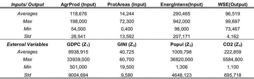
Table 1: Descriptive statistics of the inputs, external factors and the output used in the analysis.
Inputs/ Output AgrProd (Input) ProtAreas (Input) EnergIntens(Input) WSE(Output)
Averages 118,676 14,244 290,465 96,519
Max 198,000 72,300 942,000 99,697
Min 54,000 0,400 98,000 73,467
Std 28,541 13,592 207,171 4,162
External Variables GDPC (Z1) GINI (Z2) Popul (Z3) CO2 (Z4)
Averages 8938,915 40,725 1009,798 222,859
Max 33939,000 60,700 36820,000 5584,800
Min 501,000 19,500 1,306 1,100
In this study we use economic and environmental data in order to calculate
biodiversity performance of a sample of 71 countries. In that respect we need to
clarify the inputs/ outputs used. Table 1 provides descriptive statistics of the variables
used. Specifically as inputs a number of variables are used such as:
1) Total agricultural production index (1999-2001=100) (AgrProd). According
to several authors the high exposure of agricultural production in fertilisers,
pesticides, herbicides and to frequent crop rotation has resulted in into hostile habitat
for many species, which in turn have caused a decline of biodiversity on those areas
(Pimentel et al. 1992; Wagner and Edwars, 2001; Grashof-Bokdam and van
Langevelde, 2004; Billeter et al. 2008).
2) Energy intensity in all economics sectors (toe per million $) (EnergIntens).
Energy consumption due to its influence in environmental temperature levels has a
direct impact on biodiversity (Hutchinson, 1959; Wright, 1983; Allen et al., 2002;
Huston et al. 2003).
3) National protected areas (total number) in every country (ProtAreas).
According to Mcneely (1994) protected areas are essential to the conservation of
biological diversity and human welfare.
Traditional biodiversity metrics such as Shannon’s or Simpson’s index
(Simpson, 1949; Margalef, 1958) have been widely used in ecology. However, recent
approaches suggest that measurement needs to have a reference state in order to
capture the magnitude of change (Bucklandet al., 2005; Loh et al., 2005; Nielsen et
al., 2007). Lamb et al. (2009) suggest that his kind of indexes can be applied as
common metric and thus changes in biodiversity intactness can be examined. Another
issue regarding those indexes is the ecological state variables of richness and
available information which describes biodiversity. Based on the same notion this
study uses one output in a form of a weighted species enrichment (WSE) ratio. It has a
simplistic form and is calculated by the number of species known minus those which
are endangered. The species used contain full data on reptiles, mammals, fish, birds
and plants for each country. More analytically the index can be constructed as:
100
1
1 x
kij tij kij
WSE n
i n
i
(1),
where k= the number of known species, i = the country for which the species are
reported, j = is a particular specie category (i.e. plants) and t = the number of threaten
species. The higher the values of index the higher will be the country’s specie
enrichment.
According to van Strien et al. (2009) biodiversity measures need to reflect
changes in general rather than the ups and downs of particular species or species
groups. Thus it is essential to know how external ‘uncontrollable’ environmental
drivers influence the specific set of species monitored (directly or indirectly). As such
we use four other variables as external factors in order to establish their influence on
countries’ biodiversity performance. These are the data provided for population (in
thousands) (Popul), the per capita CO2 emissions (in tons CO2 per million $) (CO2), the per capita Gross Domestic Product (GDPC) and the GINI index of income
inequality (0= perfect equality). The data used in our study refer to the year 2004 for
existing species and 2003 for endangered species. Our sample consists of 71
countries2. Table 1 presents the descriptive statistics of all the variables used and as can be realised there are many disparities among the countries under consideration.
This can be justified due to the fact that the sample consists under develop and
developed countries. This can be easily observed when looking at the values of
standard deviations of the external variables, which are in our main interest when
evaluating their influence on countries’ biodiversity performance.
3. Methodology
3.1 Performance measurements
The first DEA estimator was introduced by Farrell (1957) to measure technical
efficiency. However DEA became more popular when was introduced by Charnes et
al. (1978) to estimate and allowing constant returns to scale (CCR model). The
production set constraints the production process and is the set of physically
attainable points (x,y) :
x can produce y y
x, N M (2),
where x N
is the input vector and y M
is the output vector. Later, Banker et al.
(1984) introduced a DEA estimator allowing for variable returns to scale (BCC
model). The CCR model uses the convex cone of FDH
to estimate, whereas the
BCC model uses the convex hull of FDH
to estimate. In this paper we use input
oriented models since the decision maker through different governmental policies
have greater control over the inputs compared to the outputs used. Following the
notation by Simar and Wilson (2008), the CCR model developed by Charnes et al.
(1978) can be calculated as:
n i that such for x x y y y x i n n i nThe BBC model developed by Banker et al. (1984) allowing for variable returns to
scale can then be calculated as:
n i that such for x x y y y x i n i i n n i ni i i i i M N VRS ,... 1 , 0 ; 1 ,... ; , 1 1 1 1 (4).
Finally the FDH estimator FDH
which is the free disposal hull of the observed
sample Xnand developed by Deprins et al. (1984) can be expressed as:
n i
i y X
x i i
q p n i i i i M N FDH x x y y y x X y x x x y y y x ) , ( , , , ( , , , (5).
3.2 Bias correction using the bootstrap technique
According to Simar and Wilson (1998, 2000, 2008) DEA estimators were
shown to be biased by construction. They introduced an approach based on bootstrap
techniques (Efron 1979) to correct and estimate the bias of the DEA efficiency
indicators. Therefore, the bootstrap bias estimate for the original DEA estimator
) , (x y DEA
can be calculated as:
B b DEA b DEA DEAB x y B x y x y
BIAS
1 , *
1 ( , ) ( , )
) ,
(
(6).
Furthermore, *DEA,b(x,y)
are the bootstrap values and B is the number of bootstrap
reputations. Then a biased corrected estimator of (x,y) can be calculated as:
B b b DEA DEA DEA B DEADEA x y x y BIAS x y x y B x y
1 , *
1 ( , )
) , ( 2 ) , ( ) , ( ) , (
However, according to Simar and Wilson (2008) this bias correction can create an
additional noise and the sample variance of the bootstrap values *DEA,b(x,y)
need to
be calculated. The calculation of the variance of the bootstrap values is illustrated
below:
B b B b b DEA bDEA x y B x y
B 1 2 1 , * 1 , * 1 2 ) , ( ) , (
(8).
According to Simar and Wilson (2008) we need to avoid the bias correction
illustrated in (7) unless:
3 1 )) , ( (
x y
BIASB DEA
(9).
Finally, the (1) x 100 - percent bootstrap confidence intervals can be obtained
for (x,y)as:
* 2 / * 2 /
1 ( , )
1 ) , ( ) , ( 1 a DEA a
DEA x y nc
y x nc y x
(10).
Furthermore, using the methodology proposed by Badin and Simar (2004) we obtain a
bias corrected FDH estimator:
) ( ) 1 ( ) ( 1
1 1 ()
) 1 (
y y
y n i y i y i n y y
n x x
n i x
y
x (11),
the first term is the FDH estimator and the second term is the bias correction.
According to Badin and Simar (2004) this estimator is a symmetric version of the
order-m minimum input function proposed by Cazals, Florens and Simar (2002).
Another approach is also provided by Jeong and Simar (2006) producing an algorithm
for a linearized version of FDH (LFDH) offering in such a way a bias-corrected
3.3 Testing for returns to scale and convexity
According to Simar and Wilson (2002) bootstrap techniques can be used in
order to test for the adoption of results between the Constant Returns to Scale (CRS)
against the Variable Returns to Scale (VRS) such as: :
0
H is globally CRS
against :
1
H is VRS. The test statistic mean of the ratios of the efficiency scores is
then provided by:
n i i i n VRS i i n CRS n Y X Y X n X T 1 , , ) , ( ) , ( 1 ) ( (12).Then the p-value of the null-hypothesis can be obtained as:
) )
(
(T X T H0 is true
prob value
p n obs
(13) where Tobs is the value of T computes on the original observed sample
n
X .Then this p-value can be approximated by the proportion of bootstrap values of
b
T* less the original observed value of
obs
T such as:
B b obs b B T T value p 1 * (14).According to Daraio and Simar (2005a) a similar statistical test can be created
for testing convexity between the DEA and FDH estimators. Then the null hypothesis
of convexity will be rejected if the test statistic is too small. According to Daraio and
Simar, bootstrap techniques (introduced by Simar and Wilson 1998, 2000) and are the
only way to perform these tests when evaluating the appropriate p-values. Therefore,
we use for the first time a similar approach as described previously in such a way that
:
0
H is globally CRS against :
1
H is FDH. The test statistic mean of the ratios
n i i i n FDH i i n CRS n Y X Y X n X T 1 , , ) , ( ) , ( 1 ) ( (15).Then the p-value can be calculated following equations (13) and (14). If the p-value is
too small then the FDH estimator need to be adopted against the DEA estimator since
the convexity hypothesis is not true for the original observed sample Xn.
3.4 Testing the effect of external ‘environmental’ factors on the efficiency scores
In order to analyse the effect of external variables (population, GDP per
capita, GINI index and CO2) on the efficiency scores obtained we follow the probabilistic approach developed by Daraio and Simar (2005b, 2007). They suggest
that the joint distribution of (X,Y) conditional on the environmental factor Z=z
defines the production process if Z=z. The efficiency measure can then be defined as:
inf , 0
) ,
(x yz FX xy z
(16), where
xy z
ob
X xY y Z z
Fx , Pr , . Daraio and Simar then suggested a kernel
estimator defined as follows:
y y Kz z h I h z z K y y x x I z y x F i n i i n
i i i i
n Z Y X / / , , 1 1 , ,
(17), whereK(.) is the Epanechnikov kernel and h is the bandwidth of appropriate size3. Therefore, we obtain a conditional DEA efficiency measurement defined as:
0 , inf,yz F , , xy z
x XYZn
DEA
(18).
Then in order to establish the influence of an environmental variable on the efficiency
scores obtained a scatter of the ratios
x y z y x n n , , against Z (in our case as mentioned
there are four external factors) and its smoothed nonparametric regression lines would
help us to analyse the effect of Z on the efficiency scores. If this regression is
increasing it indicates that Z is unfavourable to the efficiency of the prefectures
[image:13.595.51.595.232.777.2]whereas if it is decreasing then it is favourable.
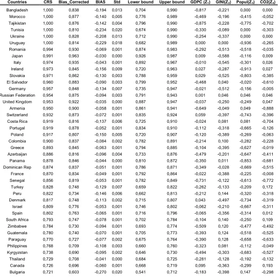
Table 2: Efficiency scores, biased corrected estimates, confidence intervals and n
x,yz
n x,y
differences of the
different external factors.
Countries CRS Bias_Corrected BIAS Std Lower bound Upper bound GDPC (Z1) GINI(Z2) Popul(Z3) CO2(Z4)
Mexico 0,718 0,668 -0,104 0,005 0,603 0,714 -0,227 0,200 -0,101 0,197 Algeria 0,714 0,637 -0,170 0,012 0,555 0,708 -0,320 -0,241 -0,308 -0,010 Korea, Rep 0,712 0,669 -0,089 0,003 0,615 0,707 -0,057 -0,357 -0,236 0,272 Malaysia 0,702 0,667 -0,074 0,002 0,622 0,697 -0,122 0,020 -0,361 -0,199 United States 0,696 0,672 -0,051 0,001 0,650 0,691 0,090 -0,111 0,000 0,065 Australia 0,693 0,619 -0,171 0,004 0,590 0,684 0,035 -0,253 -0,382 0,068 Cote d'Ivoire 0,689 0,665 -0,052 0,001 0,642 0,685 -0,583 -0,202 -0,407 -0,563 Brazil 0,680 0,630 -0,118 0,004 0,584 0,675 -0,091 0,240 0,006 0,056 Uzbekistan 0,672 0,557 -0,307 0,026 0,481 0,664 -0,430 0,086 -0,240 -0,070 Indonesia 0,667 0,629 -0,090 0,002 0,602 0,661 -0,424 -0,308 -0,020 -0,071 Chile 0,667 0,618 -0,118 0,003 0,580 0,661 -0,111 0,120 -0,414 -0,014 Cameroon 0,663 0,625 -0,092 0,002 0,588 0,656 -0,546 0,002 -0,409 -0,624 Honduras 0,652 0,621 -0,076 0,001 0,597 0,645 -0,471 0,066 -0,526 -0,561 Pakistan 0,640 0,615 -0,063 0,001 0,585 0,636 -0,520 -0,332 -0,055 -0,069 Nicaragua 0,638 0,619 -0,050 0,001 0,596 0,635 -0,491 0,103 -0,564 -0,568 Kenya 0,633 0,591 -0,112 0,002 0,560 0,624 -0,576 -0,012 -0,214 -0,442 Egypt 0,618 0,584 -0,096 0,002 0,550 0,613 -0,362 -0,334 -0,147 0,065 Ecuador 0,612 0,596 -0,045 0,001 0,574 0,609 -0,386 -0,078 -0,395 -0,356 Bolivia 0,602 0,582 -0,058 0,001 0,554 0,600 -0,453 -0,063 -0,452 -0,412 Trinidad and Tobago 0,596 0,554 -0,129 0,005 0,505 0,590 -0,048 -0,067 -0,594 -0,320 Jordan 0,575 0,538 -0,121 0,006 0,491 0,570 -0,309 -0,183 -0,524 -0,337 Venezuela 0,574 0,546 -0,090 0,002 0,517 0,571 -0,227 0,078 -0,243 -0,102 Nepal 0,570 0,528 -0,139 0,004 0,502 0,566 -0,507 -0,155 -0,279 -0,526 Jamaica 0,570 0,535 -0,116 0,002 0,508 0,563 -0,296 -0,115 -0,561 -0,374 Mozambique 0,563 0,509 -0,190 0,005 0,480 0,558 -0,534 -0,121 -0,319 -0,548 Ghana 0,557 0,478 -0,296 0,022 0,422 0,551 -0,422 -0,049 -0,290 -0,449 Zambia 0,536 0,449 -0,360 0,035 0,392 0,531 -0,513 0,160 -0,311 -0,526 Vietnam 0,530 0,484 -0,182 0,010 0,437 0,525 -0,409 -0,145 -0,104 -0,108 Tanzania, United Rep 0,519 0,462 -0,238 0,017 0,416 0,512 -0,507 -0,040 0,209 -0,500 Nigeria 0,491 0,460 -0,135 0,007 0,423 0,487 -0,454 0,080 -0,027 -0,178
Averages 0,777 0,715 -0,115 0,005 0,661 0,770 -0,282 -0,140 -0,340 -0,244 Std 0,154 0,137 0,069 0,007 0,128 0,152 0,233 0,210 0,273 0,277 Max 1,000 0,963 -0,030 0,035 0,926 0,990 0,095 0,240 0,209 0,272 Min 0,491 0,449 -0,360 0,000 0,392 0,487 -0,875 -0,588 -0,936 -0,888
4. Empirical results
Following the methodology proposed by Simar and Wilson (2002) this paper
tests the model for the existence of returns to scale (analysed previously). In our
application we have three input factors and one output and we obtained for this test a
p-value of 0,98 > 0,05 (with B=2000) hence, we cannot reject the null hypothesis of
assuming constant returns to scale4. Furthermore, we obtained a similar statistical test for assuming convexity on the results obtained and thus to choose between the CCR
and FDH estimates (bias corrected). In a process analysed previously we obtained a
p-value of 0,77 > 0,05 (with B=2000) hence, we cannot reject the null hypothesis of
CRS.
Overall, the tests indicate that the proper estimates for measuring countries’
biodiversity performances are obtained by the CCR model. The efficiency results
obtained using the methodology proposed are presented in table 2. Analytically, table
2 presents the efficiency scores of the 71 countries, the biased corrected efficiency
scores and the 95-percent confidence internals: lower and upper bound obtained by
B=2000 bootstrap replications using the algorithm described previously. As reported
the biodiversity efficient countries (i.e. efficient score =1) are reported to be
Bangladesh, Marocco, Tajikistan, Tunisia, Ukraine and Uruguay. Whereas countries
with higher scores (i.e. more than 0,8) are reported to be Romania, Japan, Italy,
Ireland, Slovakia, El Salvador, Germany, Russian Federation, the United Kingdom,
Armenia, Switzerland, Costa Rica, Portugal, Poland, Colombia, Greece, Azerbaijan,
Panama, Dominican Rep, France, Senegal, Turkey, Peru, Denmark, Israel and Spain.
Finally, the countries with the lowest performance (<0,6) are Trinidad and Tobago,
Jordan, Venezuela, Nepal, Jamaica, Mozambique, Ghana, Zambia, Vietnam, Tanzania
United Rep. and Nigeria. However, these results obtained from biased CCR indicators
and as explained previously following expression (9) the biased corrected results need
to be adopted for our analysis. According to the biased corrected efficiency measures
the countries with the higher biodiversity efficiency scores (i.e. > 0,8) are reported to
be Japan, Italy, Romania, the United Kingdom, Armenia, El Salvador, Portugal,
Morocco, Tajikistan, Russian Federation, Switzerland, Slovakia, Germany, Panama,
Greece, Ireland, Bangladesh, Colombia, Dominican Rep, France, Ukraine, Senegal,
Costa Rica, Azerbaijan, Uruguay, Tunisia and Poland. Furthermore, the countries with
poor performance (i.e. <0.6) are Trinidad and Tobago, Venezuela, Jordan, Jamaica,
Nepal, Mozambique, Vietnam, Ghana, Tanzania United Rep., Nigeria and Zambia.
Adopting the methodology proposed before we created four conditional CCR
biodiversity efficiency estimators taking into account the influence of the four
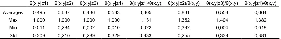
[image:16.595.61.527.320.386.2]external variables used (i.e. population, GDPC, GINI and CO2). Table 3: Descriptive statistics of the conditional DEA estimates
θ(x,y|z1) θ(x,y|z2) θ(x,y|z3) θ(x,y|z4) θ(x,y|z1)/θ(x,y) θ(x,y|z2)/θ(x,y) θ(x,y|z3)/θ(x,y) θ(x,y|z4)/θ(x,y) Averages 0,495 0,637 0,436 0,533 0,605 0,831 0,558 0,664
Max 1,000 1,000 1,000 1,000 1,131 1,352 1,404 1,382 Min 0,011 0,284 0,002 0,010 0,022 0,392 0,004 0,018 Std 0,309 0,210 0,289 0,329 0,333 0,255 0,339 0,381
Table 3 provides the descriptive statistics of the several conditional DEA
estimators used5. As can be realised the highest influence on countries biodiversity performance is due to countries’ population. The original average value of the
efficiency scores (Table 2) was 0,777 (for the biased efficiency scores) and 0,715 (for
the unbiased efficiency scores). However taking into account the influence of the
countries’ populations, the average value of the efficiency score has been decreased to
the level of 0,436 (Table 3). Similarly the next higher effect has been made by the
countries’ levels of GDP per capita. The influence of GDP per capita on countries’
biodiversity performance has decreased the average efficiency scores to 0,495.
Accordingly the levels of countries’ CO2 have decreased countries’ efficiency scores to an average value of 0,533. However, the GINI index doesn’t seem to have such a
dramatic influence on countries’ biodiversity performance compared to the other three
variables examined. The same conclusions can be obtained when analysing the
descriptive statistics of the ratios of conditional DEA to the original DEA estimates
[image:17.595.85.511.179.502.2]θ(x,y|z)/θ(x,y).
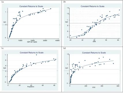
Figure 1: Examining the effect of the external variables on countries’ biodiversity performance
1a 1b
1c 1d
As described previously figure 1 illustrates the effect of the three external
variables on countries’ biodiversity performance. As can be realised by the graphs
(1a-d) the four factors have a negative effect on countries’ performances. However,
one of the interesting points of this study is to analyse the effect of the four factors on
a country to country basis. For that reason the result of the efficiency levels of θ(x,y) -
θ(x,y|z) are presented on Table 2 according to the external factors. Analysing the
results on Table 2 we can observe that GDP per capita has a positive influence on
several countries’ biodiversity performances. These countries are Canada, the United
0 .2 .4 .6 .8 1
Qz3
0 20 40 60 80
Population
Constant Returns to Scale
0 .5 1 1.5
Qz4
0 200 400 600
CO2
Constant Returns to Scale
.4 .6 .8 1 1.2 1.4
Qz2
20 30 40 50 60
GINI
Constant Returns to Scale
0 .5 1
Qz1
0 10000 20000 30000 40000
GDP per capita
States, Switzerland, Denmark, Australia, Slovakia, Ireland and Japan. However, for
some countries GDP per capita has a negative impact. The highest negative impact
levels on countries’ biodiversity performances (> -0,5) have been reported for Nepal,
Tanzania United Rep, Zimbabwe, Zambia, Pakistan, Mozambique, Cameroon, Kenya,
Cote d'Ivoire, Armenia, Senegal, Bangladesh and Tajikistan.
Furthermore, when we are looking at the effect of income inequality (GINI) on
countries biodiversity performance we realise that it has a small positive effect on
countries’ performance. These countries are Brazil, Mexico, Zambia, Peru, South
Africa, Paraguay, Guatemala, Chile, Zimbabwe, Nicaragua, Colombia, Uzbekistan,
Costa Rica, Philippines, Nigeria, Venezuela, Honduras, Russian Federation, El
Salvador, Malaysia, Panama and Cameroon. However, income inequality has a
negative effect on countries’ performance with the highest negative results (> -0,5) to
be reported for Denmark, Germany, Romania, Slovakia, Italy and Japan.
Population appears to have a small positive impact on six countries’
biodiversity performances (Tanzania United Rep, Bulgaria, Costa Rica, Armenia,
Russian Federation and Brazil), however, on the rest of the countries it appears to
have a negative impact. The countries which appear to be affected the most (i.e.
>-0,7) are Denmark, Switzerland, Tajikistan, Slovakia, Panama, Ireland and Uruguay.
Finally, for the case of CO2 it can be realised that in the majority of cases the influence is negative. Specifically, the highest negative influence (>-0,5) is reported
for Tanzania United Rep, Dominican Rep, Guatemala, Nepal, Zambia, Kyrgyzstan,
Mozambique, Honduras, Cote d'Ivoire, Nicaragua, El Salvador, Cameroon, Paraguay,
5. Conclusions
Strien et al. (2009) have provided a typology of biodiversity indicators relative
to their link with their environmental factors based on the typology introduced by
Gregory et al. (2005). As such this study provides a composite indicator of measuring
countries’ biodiversity performance and can be characterised as ‘type 4’ indicators.
These kinds of indicators show how biodiversity is responding to environmental
factors in general, rather than looking how specific species or species groups are
doing. As such, to our knowledge, for the first time, this study uses conditional DEA,
bootstrap techniques and kernel density estimations for 71 countries in order to
measure their biodiversity performances. By obtaining among others, the efficiency
scores and the optimal ratios levels for inefficient countries this study provides raw
policy models for biodiversity performance evaluation. Following Hamilton’s (2005)
remarks regarding biodiversity’s theoretical limitations of measurement and its
usefulness in a sociological and political perspective, this paper provides a real
example of how new advances in DEA methodology can be used for providing a
methodological framework creating biodiversity indicators taking into account
different environmental factors. In addition, the methodological tests adopted revealed
that the convexity proved to be a vital issue of the construction of unbiased DEA
estimators. Moreover, when we test for scale efficiencies it appeared that such a
hypothesis would led us to biased estimations.
As such, the empirical results reveal that GDP per capita, income inequalities,
levels of CO2 and population level have an overall negative effect on countries’ biodiversity performance. However, countries’ population level is the dominant threat
of countries’ biodiversity performance followed up by GDP per capita and income
developed countries’ biodiversity performance but a negative effect on under develop
and developing countries. From the other hand income inequalities have a negative
effect on developed countries’ biodiversity performance and a positive effect on under
develop and developing countries. The results reveal, that CO2, population, income inequalities and GDP per capita have different impact on developed, under develop
and developing countries and therefore environmental policies must be adopted and
implemented accordingly.
Due to the fact that the main concerns of the environmental social sciences is
the deep understanding of the social and economic forces that change the environment
the methodological approach applied in this paper can be a vital tool for shaping and
References
Allen, A.P., Brown, J.H., Gillooly, J.F., 2002. Global biodiversity, biochemical
kinetics, and the energetic-equivalence rule. Science 297, 1545-1548.
Alsharif, K., Feroz, E.H., Klemer, A., Raab, R., 2008. Governance of water supply
systems in the Palestinian Territories: A data envelopment analysis approach to the
management of water resources. Journal of Environmental Management 87, 80-94.
Badin, L., Simar, L., 2004. A bias corrected nonparametric envelopment estimator of
frontiers. Discussion Paper 0406, Institut de Statistique, Universite´ Catholique de
Louvain, Louvain de la Neuve, Belgium.
Banker, R.,D., Charnes, A., Cooper, W.W., 1984. Some Models for Estimating
Technical and Scale Inefficiencies in Data Envelopment Analysis. Management
Science 30, 1078 – 1092.
Billeter, R., Liira, J., Bailey, D., Bugter, R., Arens, P., Augenstein, I., Aviron, S.,
Baudry, J., Bukacek, R., Burel, F., Cerny, M., De Blust, G., De Cock, R., Diekotter,
T., Dietz, H., Dirksen, J., Dormann, C., Durka, W., Frenzel, M., Hamersky, R.,
Hendrickx, F., Herzog, F., Klotz, S., Koolstra, B., Lausch, A., Le Coeur, D., Maelfait,
J.P., Opdam, P., Roubalova, M., Schermann, A., Schermann, N., Schmidt, T.,
Schweiger, O., Smulders, M.J.M., Speelmans, M., Simova, P., Verboom, J., van
Wingerden, W.K.R.E., Zobel, M., Edwards, P.J., 2008. Indicators for biodiversity in
agricultural landscapes: a pan-European study. Journal of Applied Ecology 45,
141-150.
Buckland, S.T., Magurran, A.E., Green, R.E., Fewster, R.M., 2005. Monitoring
change in biodiversity through composite indices. Philosophical Transactions of the
Cazals, C., Florens, J.P., Simar, L., 2002. Nonparametric frontier estimation: a robust
approach. Journal of Econometrics 106, 1-25.
Charnes, A., Cooper, W.W., Rhodes, L.E., 1978. Measuring the efficiency of decision
making units. European Journal of Operational Research 2, 429-444.
Daraio, C., Simar, L., 2005a. Conditional Nonparametric frontier models for convex
and non convex technologies: a unifying approach. Working Paper 2005/12
Laboratory of Economics and Management LEM Pisa, Italy.
Daraio, C., Simar, L., 2005b. Introducing environmental variables in nonparametric
frontier models: A probabilistic approach. Journal of Productivity Analysis 24, 93–
121.
Daraio, C., Simar, L., 2007. Advanced robust and nonparametric methods in
efficiency analysis. Springer Science, New York.
Delong, B., 2003. Estimating world GDP, one million B.C.-present. Department of
Economics, University of California, Berkley.
Derpin, D., Simar, L., Tulkens, H., 1984. Measuring labor efficiency in post offices,
in: Marchand, M., Pestieau, P., Tulkens, H. (Eds), The performance of public
enterprises: Concepts and measurement. Amstredam: North-Holland, pp. 243-267.
Efron, B., 1979. Bootstrap methods: another look at the jackknife. The Annals of
Statistics 7, 1-16.
Färe, R., Grosskopf, S., Hernandez-Sancho, F., 2004. Environmental performance: an
index number approach. Resource and Energy Economics 26 (4), 343-352.
Färe, R., Grosskopf, S., Sancho, H., 1999. Environmental performance: an index
number approach. Department of Economics Working Paper. Oregon State
Färe, R., Grosskopf, S., Zaim, O., 2003. An Environmental Kuznets Curve for the
OECD countries. In: Färe, R., Grosskopf, S. (Eds.), New Directions: Efficiency and
Productivity. Kluwer Academic Publishers, pp. 79–90.
Farrell, M.J., 1957. The Measurement of Productive Efficiency. Journal of the Royal
Statistical Society 120, 253-281.
Grashof-Bokdam, C.J., van Langevelde, F., 2004. Green veining: landscape
determinants of biodiversity in European agricultural landscapes. Landscape Ecology
20, 417–439.
Gregory, R.D., van Strien, A.J., Vorisek, P., Gmelig Meyling, A.W., Noble, D.,
Foppen, R.P.B., Gibbons, D.W., 2005. Developing indicators for European birds.
Philosophical Transactions of the Royal Society B 360, 269–288.
Halkos, G.E., Tzeremes, N.G., 2009. Exploring the existence of Kuznets curve in
countries' environmental efficiency using DEA window analysis. Ecological
Economics doi:10.1016/j.ecolecon.2009.02.018.
Hamilton, A.J., 2005. Species diversity or biodiversity? Journal of Environmental
Management 75, 89-92.
Hoffman, J., 2004. Social and environmental influences on endangered species: a
cross-national study. Sociological Perspectives 47, 79-107.
Huston, M.A., Brown, J.H., Allen, A.P., Gillooly, J.F., 2003. Heat and biodiversity.
Science 299, 512-513.
Hutchinson, G.E., 1959. Homage to Santa Rosalia or why are there so many kinds of
animals. American Naturalist 93, 145-159.
Jeong, S.O., Simar, L., 2006. Linearly interpolated FDH efficiency score for
Jung, E.J., Kim, J.S., Rhee, S.K., 2001. The measurement of corporate environmental
performance and Its application to the analysis of efficiency in oil industry. Journal of
Cleaner Production 9(6), 551-563.
Kao, C., Chhang, P.L., Hwang, S.N., 1993. Data envelopment analysis in measuring
the efficiency of forest management. Journal of Environmental Management 38,
73-83.
Lamb, E., G., Bayne, E., Holloway, G., Shieck, J., Boutin, S., Herbers, J., Haughland,
D.L., 2009. Indices for monitoring biodiversity change: Are some more effective than
others? Ecological Indicators 9, 432-444.
Loh, J., Green, R.E., Ricketts, T., Lamoreux, J., Jenkins, M., Kapos, V., Randers, J.,
2005. The living planet index: using species population time series to track trends in
biodiversity. Philosophical Transactions of the Royal Society B 360, 289–295.
Magurran, A.E., 2004. Measuring Biological Diversity. Blackwell, Oxford.
Margalef, R.D., 1958. Information theory in ecology. General Systems 36–71.
McNeely, J.A., 1994. Protected areas for the 21st century: working to provide benefits
to society. Biodiversity and Conservation 3,390-405.
Nielsen, S.E., Bayne, E.M., Schieck, J., Herbers, J., Boutin, S., 2007. A new method
to estimate species and biodiversity intactness using empirically derived reference
conditions. Biological Conservation 137, 403–414.
Pimentel, D., Acquay, H., Biltonen, M., Rice, P., Silva, M., Nelson, J., Lipner, V.,
Giordano, S., Horowitz, A., D'Amore M., 1992. Environmental and economic costs of
pesticide use. BioScience 42(10), 750- 760.
Simar, L., Wilson, P., 2008. Statistical interference in nonparametric frontier models:
measurement of productive efficiency and productivity change, Oxford University
Press, New York.
Simar, L., Wilson, P.W., 1998. Sensitivity analysis of efficiency scores: how to
bootstrap in non parametric frontier models. Management Science 44, 49-61.
Simar, L., Wilson, P.W., 2000. A general methodology for bootstrapping in
non-parametric frontier models. Journal of Applied Statistics 27, 779 -802.
Simar, L., Wilson, P.W., 2002. Non parametric tests of return to scale. European
Journal of Operational Research 139, 115-132.
Simpson, E.H., 1949. Measurement of diversity. Nature 163, 688.
Taskin, F., Zaim, O., 2000. Searching for a Kuznets curve in environmental efficiency
using kernel estimations. Economics Letters 68, 217–223.
Turner, R.K., Button, K., Nijkamp, P., 1999. Ecosystems and Nature: Economics,
Science and Policy. Elgar, Cheltehham.
Tyteca, D., 1996. On the measurement of the environmental performance of firms e a
literature review and a productive efficiency perspective. Journal of Environmental
Management 46 (3), 281-308.
Tyteca, D., 1997. Linear programming models for the measurement of environmental
performance of firms e concepts and empirical results. Journal of Productivity
Analysis 8 (2), 183-197.
Van Strien, A.J., van Duuren, L., Foppen, R.P.B., Soldaat, L.L., 2009. A typology of
indicators of biodiversity change as a tool to make better indicators. Ecological
Indicators doi:10.1016/j.ecolind.2008.12.001.
Wagner, H.H., Edwards, P.J., 2001. Quantifying habitat specificity to assess the
contribution of a patch to species richness at a landscape scale. Landscape Ecology
World Resource Institute (WRI), United Nations Development Programme (UNDP),
The World Bank (2005), World Resources 2003-2004. Oxford University Press, New
York.
Wright, D.H., 1983. Species-energy theory: an extension of species-area theory.
Oikos 41, 496-506.
Zaim, O., Taskin, F., 2000. A Kuznets curve in environmental efficiency: an