Munich Personal RePEc Archive
Expectations-Driven Cycles in the
Housing Market
Lambertini, Luisa and Mendicino, Caterina and Punzi,
Maria Teresa
22 October 2010
Online at
https://mpra.ub.uni-muenchen.de/26254/
Expectations-Driven Cycles in the Housing Market
∗Luisa Lambertini† Caterina Mendicino‡ Maria Teresa Punzi§
October 22, 2010
Abstract
This paper analyzes housing market boom-bust cycles driven by changes in households’ expectations. We explore the role of expectations not only on productivity but on several other shocks originated in the housing market, the credit market, the production sector and the conduct of monetary policy. We find that expectations related to different sectors of the economy can generate booms in the housing market in accordance with the empirical findings. However, only expectations of future expansionary monetary policy that are not fulfilled can also generate a macroeconomic recession. Regarding the credit market, increased access to credit generates boom-bust cycles only if it is expected to be reversed in the near future. Moreover, economies with higher access to credit are characterized by higher volatility of consumption and indebtedness but, not necessarily, of real GDP.
∗The opinions expressed in this article are the sole responsibility of the authors and do not necessarily reflect
the position of the Banco de Portugal or the Eurosystem. We are grateful to seminar participants at the Banco
de Espa˜na, the Banco de Portugal, Universidade Nova de Lisboa, Catholic University of Louvain, the University of
Surrey, the meeting of the Society of Economic Dynamics, the 2010 meeting of the 16th International Conference on
Computating in Economics and Finance and the European Economic Association 2010 Congress for useful feedbacks
on this project. We also thank Isabel Correia, Daria Finocchiaro, Matteo Iacoviello, Nobuhiro Kiyotaki, Stefano
Neri, Eva Ortega and Joao Sousa for valuable comments and suggestions. The last author acknowledge the Banco
de Portugal for the 2009 visiting research grant.
†EPFL, College of Management. Email: luisa.lambertini@epfl.ch
1
Introduction
Boom-bust cycles in asset prices and economic activity are a central issue in policy and academic debates. Particular attention has been given to the behavior of housing prices and housing in-vestment. This paper suggests a mechanism for modeling housing-market boom-bust cycles in accordance with the empirical pattern. We document that, over the last three decades, housing prices boom-bust cycles in the United States have been characterized by co-movement in GDP, consumption, investment, hours worked, real wages and housing investment. Moreover, housing prices peaks are often followed by macroeconomic recessions.
Modeling endogenous boom-bust cycles in macroeconomics is a major challenge. An often-heard explanation of housing booms is optimism about future house price appreciation. It is plausible to think that optimism about house prices is related to current or expected macroeconomic developments. Our explanation builds on a “news shock” mechanism where public signals of future fundamentals cause business cycle fluctuations through changes in household expectations. Booms are generated by public signals; busts follow if the signals are not realized ex-post. To this purpose, we extend the model of the housing market developed by Iacoviello and Neri (2009) to include expectations of future macroeconomic developments. We rely on their estimated model since it is rich enough to explore the role of alternative sources of optimism about future house prices originating from developments in different sectors of the economy: the credit market, the housing market, the production sector and the conduct of monetary policy.
This paper provides several insightful results. We document that unanticipated shocks fail in generating either hump-shaped dynamics or the observed co-movement among hours worked, investment, GDP and house prices. A necessary condition for a boom to emerge is that agents expect a future increase in housing prices, which fuels current housing demand and lifts housing prices immediately. The increase in housing prices is coupled with an endogenous increase in household indebtedness, which stems from the fact that households borrow a fraction of the future expected value of their houses. Busts occur if expectations are not fulfilled, which implies a dramatic drop in both aggregate quantities and prices. Accordingly, several types of expectation-driven cycles can generate fluctuations in the housing market. Changes in expectations about future productivity, investment costs, housing supply, inflation, the policy rate and the central bank’s target can generate housing-market boom-bust cycles characterized by co-movement in GDP, consumption, investment, hours and real wages. However, only expectations of future expansionary monetary policy that are not met are likely to cause a boom-bust cycle and a subsequent macroeconomic recession.
the model, the increase in housing prices generated by changes in expectations is always coupled with an endogenous increase in household indebtedness. However, improvement in the access to credit per se is often considered as one of the main drivers of housing booms. We document that an exogenous easing of credit conditions generates boom-bust cycle dynamics only if the current favorable situation in the credit market is expected to be reversed in the near future.
Since Beaudry and Portier (2004, 2007), a growing strand of the business cycle literature inves-tigated the role of changes in expectations or news about the future state of productivity as a source of business cycle fluctuations. Changes in expectations may prove to be an important mechanism in creating business cycle fluctuations if they generate pro-cyclical movements in consumption, hours and investment. However, as already shown by Beaudry and Portier (2004, 2007), a stan-dard one-sector real business cycle model is unable to generate boom-bust cycles in response to news. This is due to the wealth effect generated by expectations of improved future macroeconomic conditions that make consumption increase and hours worked fall at the time of the signal. Several papers explore the role of alternative modeling features in the transmission of expectations-driven cycles. Christiano, Ilut, Motto, and Rostagno (2008) show that for the price of capital to be posi-tively correlated with all other aggregate variables, an inflation targeting central bank and nominal wages stickier than prices are needed. Differently from previous studies we aim at reproducing empirically plausible boom-bust cycles in the housing market. We document that expectations on future productivity generate business cycle fluctuations in a model of the housing market that fea-tures collateralized household debt, standard preferences and production functions, and standard assumptions about nominal rigidities, both in prices and wages.
Compared to previous literature, a novel element in this paper is the introduction of changes in expectations on shocks related to the conduct of monetary policy or developments in the credit and housing market. We also study the role of credit market development in economies subject to boom-bust cycles. We analyze how the degree of credit market development affects the the long-run properties of the model, the transmission of news shocks and the implied volatility. At the steady state, economies with a lower degree of credit frictions are characterized by higher aggregate consumption, investment and GDP. Credit market conditions also play an important role in the transmission of expectations-driven cycles. Economies characterized by easier access to credit have higher volatility of aggregate consumption and household indebtedness but not necessarily of GDP if variations in relative prices enter its measurement.
productiv-ity shocks, easier access to credit imply lower volatilproductiv-ity of output, consumption, and hours worked. According to their findings, the U.S. mortgage market liberalization of the early 1990s played a role in explaining the great moderation. On the other hand, Calza, Monacelli and Stracca (2009) show that the transmission of monetary policy shocks to residential investment and consumption is stronger for lower values of the down-payment ratio. This literature however abstracts from the possibility of expectations-driven fluctuations. In particular, none of these papers analyzes the re-lationship between credit market developments and the occurrence and impact of boom-bust cycles in the housing market.
It is important to stress that the goal of this paper is not to explain exactly what happened in a specific country, but to draw qualitative conclusions on the plausibility of changes in expectations as a mechanism to generate boom-bust cycles in the housing market. However, given the robustness of the results to different model’s parameters, our findings can be generalized to any industrialized country.
The rest of the paper is organized as follows. Section 2 characterizes the average behavior of several macroeconomic variables during four boom-bust episodes in the U.S. housing market in the last four decades. Section 3 describes the model. Section 4 studies the dynamics of the model under unexpected shocks and Section 5 investigates the occurrence of boom-bust cycles in the housing market as a consequence of expectations regarding future macroeconomic developments. Section 6 analyzes the role of credit market development on the steady state and volatility of the economy. Section 7 concludes.
2
Stylized Facts about Housing Boom-Bust Episodes and the
Macro-economy
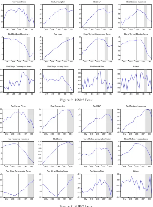
Real house prices also display a number of boom-bust episodes, namely periods of faster-than-trend growth followed by sharp reversals. We define a peak as the centered maximum in real house prices in a twenty-one-quarters window, excluding end points. Using this definition, we identify four peaks in real house prices in the United States: 1973:3; 1979:4; 1989:2; 2006:2. The vertical
lines in Figure 1 indicate the peak dates.1 Our definition of peak is robust to de-trending, either
with a linear trend or with an Hodrick-Prescott filter.2
Interestingly, real house prices peaks are followed by macroeconomic recessions. The grey shaded
areas in Figure 1 indicate recession dates according to the National Bureau of Economic Research.3
Every housing peak as defined above has been followed by an economic downturn. Even the housing price high of 1969:4, which does not qualify as a peak according to our definition because real house prices rebounded too quickly, was followed by a recession.
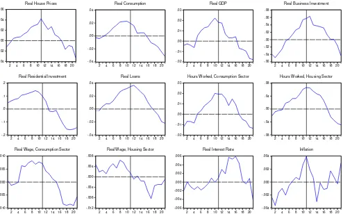
We are interested in characterizing the behavior of our macroeconomic variables during these four boom-bust episodes. First we consider the average behavior of our macroeconomic variables over the four peak episodes. Figure 2 shows the average behavior of these series in the twenty-one quarter window around a peak date. The vertical line indicates the peak in real house prices.
On average real house prices are pro-cyclical during boom-bust episodes. In fact, real house prices peak when real GDP reaches a maximum. Figures 4 to 7 illustrate the behavior of the macroeconomic variables of interest in each peak episode. Real personal consumption also increases during the boom in real house prices and peaks around the same time as the peak in real GDP and house prices. Real private residential investment reaches its maximum before the peak in house prices and falls rapidly afterward. On the other hand, real private nonresidential investment increases during the boom period, peaks after the peak in housing prices and falls afterward. Hours worked follow closely the dynamics of real house prices, both in the construction and in the consumption-good sector.
1A more stringent definition would require the peak to be the high of a longer centered window. For example, if
we require the window to be twenty-five quarters, as in Ahearne et al. (2005), the 1973:3 high in real house prices
would fail to be a peak. In general, upward trending house prices make it difficult to identify peaks in long, centered
windows because prices do not fall all the way to the levels they had at the beginning of the boom. On the other
hand, a shorter centered window of seventeen quarters would deliver an additional peak in 1969:4.
2Using the H-P filter and the twenty-one quarters definition of window would deliver two additional peaks in
1994:1 and 1999:2, the same peaks in 1973:3, 1979:4 and 1989:2, and it would put the most recent peak in 2007:1. 3At the time the paper was written, the National Bureau of Economic Research had dated the beginning of the
recession in 2007:4 but not its end. Figure 7 assumes that the recession was not over yet as of the end of boom-bust
On average real loans grow during the boom phase and peak several quarters after the peak in housing prices. Inspection of the four peak episodes reveals that real loans typically peak at the beginning of the recession that follows the bust in housing prices. In the 1973:3 and 1979:4 episodes real GDP and real loans peak immediately after housing prices; in the 2006:2 episode real GDP and real loans peak only some quarters after housing prices. The 1989:2 housing peak is an exception, as real loans continued to grow despite a fall in housing prices. The evidence that real loans grow during the boom phase and fall during the bust phase of housing prices is in line with the findings in Kannan, Rabanal and Scott (2009), who consider several countries and find evidence of higher-than-normal growth rates of credit relative to GDP in the run-ups to house price busts since 1985. They also find large deteriorations in current account balances and higher-than-normal ratios of investment to GDP after 1985 but not before it. Further differences among peak episodes are discussed in Appendix B.
Inflation follows real house prices and other macroeconomic variables with some lags. On average, inflation increases before the peak in house prices, reaches a maximum after the peak in house prices and then falls. The real interest rate, measured by the three months Treasury bill minus inflation, increases throughout the boom period, peaks around the time of or just after the peak in house prices, and then it falls rapidly. Real wages are pro-cyclical during boom-bust episodes. Real wages in the consumption-good sector rise in the boom and fall in the bust phase. Real wages in the construction sector have a similar pattern with a couple of differences: They peak before real house prices (and real wages in the consumption-good sector) and they fall much more rapidly after that.
Next we transform our variables in deviations from the Hodrick-Prescott filter and then calculate the average over the four housing-peak episodes. This allows us to see if housing boom-bust episodes are accompanied by below- or above-trend behavior of some variables. Figure 3 shows the data. A number of observations are in order. Real house prices, real GDP, private consumption and investment, both residential and nonresidential, and real loans fall below trend at the end of the bust phase. Models featuring unanticipated shocks that eventually die away cannot reproduce this feature of the data. The real interest rate is below trend at the beginning of the boom phase, consistent with the evidence in Figure 2. This evidence is consistent with the hypothesis that housing booms have been accompanied by low real interest rates. Real wages start at or above trend, the reach a maximum before the peak in real house prices and then fall well below trend.
to 2009:2; the second column displays the same statistics over the four twenty-one quarter windows centered around the peaks identified earlier. GDP, consumption, business investment, real loans, hours and real wages become more positively correlated, or maintain the same correlation, with real house prices during boom-bust episodes. On the other hand, the real interest rate and inflation are less correlated with real house prices during boom-bust episodes. All variables except business investment are more volatile during peak episodes. The increase in volatility is substantial for real wages, inflation, residential investment, the real interest rate and consumption.
3
The Model
We adopt the model of the housing market developed by Iacoviello and Neri (2009) since it allows us to investigate the transmission mechanism of news related to the housing market, credit market, the production sector and the conduct of monetary policy on future house price appreciation. In the following, we report the main features of the model. The model’s parameters are set equal to the mean of the posterior distribution estimated by Iacoviello and Neri (2009) for the U.S. economy.
3.1 Households
The economy is populated by two types of households: the Saver and the Borrower. They both work in the good- and housing-sector of production, consume and accumulate housing. They differ
in their discount factors, (β and β′). Borrowers (denoted by′) feature a relatively lower subjective
discount factor that in equilibrium generates an incentive to anticipate future consumption to the current period through borrowing. Hence, the ex-ante heterogeneity induces credit flows between the two types of agents. This modeling feature has been introduced in macro models by Kiyotaki and Moore (1997) and extended by Iacoviello (2005) to a business cycle framework with housing investment.
The Saver maximizes the utility function with respect to :
Ut=Et
∞
X
t=0
(βGC)t
"
Γcln (ct−εct−1) +jtln ht−
τ
1 +η(n
1+ξ c,t +n
1+ξ h,t ) 1+η 1+ξ # subject to:
ct+qt
ht−(1−δh)ht−1
+ kc,t Ak,t −
1−δk
Ak,t
+Rc,tzc,t
kct−1
+φc,t+[kh,t(1−δk+Rh,tzh,t)kht−1] +
φh,t+kb,t+pl,tlt−bt+
Rt−1bt−1
πt
≤ wc,tnc,t
Xwc,t
+wh,tnh,t
Xwh,t
wherec,h ,nc and nh are consumption, housing services, hours worked in the good-sector and in
the construction-sector, respectively. The parameter ξ defines the degree of substitution between
the two sectors in terms of hours worked,4 while ηis the inverse of Frisch elasticity of labor supply.
jtdetermines the relative weight in utility of housing services,Rtis the lending interest rate,δc and
δh represent the depreciation rate for capital and housing stock, respectively. lt is the land priced
atpl,tandqtis the price of the houses, all relative to the CPI.zc,tandzh,t are the capital utilization
rates of transforming potential capital into effective capital in the two sectors. Dt are lump-sum
profits paid to households. The term Ak,t is an investment-specific technology that captures the
marginal cost of producing consumption-good-sector specific capital.5 GC,GIKc and GIKhare the
trend growth rates of real consumption and capital used in the two sectors of production. Γc and Γ
′
c
represent scaling factors of the marginal utilities of consumption. Wages are set in a monopolistic
way and can be adjusted subject to a Calvo scheme with probability 1−θw every period. Xwc,t
and Xwh,t are markups on the wages paid in the two sectors. Both households set wages in a
monopolistic way.
The Borrower maximizes the utility function:
Ut=Et
∞
X
t=0
(β′GC)t
"
Γ′cln (c
′
t−ε
′
c′t−1) +jtln h
′
t−
τ
1 +η′((n
′
c,t)1+ξ
′
+ (n′h,t)1+ξ
′ )
1+η′
1+ξ′
#
subject to:
c′t+qt
h′t−(1−δh)h
′
t−1
−b′t≤ w ′
c,tn
′
c,t
Xwc,t′ +
wh,t′ n′h,t Xwh,t′ +D
′
t−
Rt−1b ′
t−1
πt
and
b′t≤mtEt
qt+1h ′
tπt+1
Rt
β′ ∈(0, β) captures the Borrower’s relative impatience.
4For a value of ξ close to zero, hours worked in the two sectors are close to perfect substitutes, which means
that the worker would devote most of the time to the sector that pays the highest wage. Positive values ofξimply,
instead, that hours worked are far from perfect substitutes, thus the worker is less willing to diversify her working
hours across sectors even in the presence of a wage differential (see Horvath (2000) for details)
5φc,t= φkc
2GIKc
kc,t
kc,t−1 −
GIKc
2
kc,t−1
(1+γAK)t is the good-sector capital adjustment cost, andφh,t=
φkh
2GIKh
kh,t
kh,t−1
−
GIKh
2
kh,t−1 is the housing-sector capital adjustment cost; γAK represents the net growth rate of technology in
business capital, φkc andφkh indicate the coefficients for adjustment cost (i.e., the relative prices of installing the
Limits on borrowing are introduced through the assumption that households cannot borrow
more than a fraction of the next-period value of the housing stock. The fraction m, referred to as
the equity requirement or loan-to-value ratio, should not exceed one and is treated as exogenous to the model. It can be interpreted as the creditor’s overall judicial costs in case of debtor default and represents the degree of credit frictions in the economy. The borrowing constraint is consistent with standard lending criteria used in the mortgage and consumer loan markets. We explore the effects of temporary deviations from the established degree of credit market access by assuming
thatmt is stochastic. We refer to this as a loan-to-value ratio shock.
3.2 Firms
Final good producing firms produce non-durable goods (Y) and new houses (IH). Both sectors face
Cobb-Douglas production functions. The housing sector uses capital,k,land,l, and labor supplied
by the Savers,n, and the Borrowers, n′, as inputs of production.
IHt=
Ah,t
nαh,t+n′h,t1−α
1−µh−µb−µl
(zh,tkh,t−1)µhkµbbl
µl
t−1.
The non-housing sector produces consumption and business capital using labor and capital.
Yt=
Ac,t
nαc,t+n′c,t1−α
1−µc
(zc,tkc,t−1)µc.
Ah,t and Ac,tare the productivity shocks to the housing- and good-sector, respectively. Firms pay
the wages to households and repay back the rented capital to the Savers.
The intermediate good-sector is populated by a continuum of monopolistically competitive
firms owned by the Savers. Prices can be adjusted by each producer with probability 1−θπ every
period, following a Calvo-setting. Monopolistic competition occurs at the retail level, leading to the following forward-looking Philips curve:
lnπt−ιπlnπt−1=βGC
Etlnπt+1−ιπlnπt
−ǫπln(Xt/X) +up,t
whereǫπ = (1−θπ)(1−θπ βθπ), Xtrepresents the price markup andup,tis a cost-push shock. In contrast,
housing prices are assumed to be flexible.
3.3 Monetary Policy Rule
We assume that the central bank follows a Taylor-type rule as estimated by Iacoviello and Neri (2009):
Rt=Rrt−1R π
(1−rR)rπ
t
GDPt
GCGDPt−1
(1−rR)rY
rr(1−rR)uR,t
As,t
where rr is the steady-state real interest rate and uR,t is a monetary policy shock. The central
bank’s target is assumed to be time varying and subject to a persistent shock,st, as in Smets and
Wouters (2003). Following Iacoviello and Neri (2009), GDP is defined as the sum of consumption and investment at constant prices. Thus
GDPt=Ct+IKt+qIHt,
whereq is real housing prices along the balanced growth path.
3.4 News Shocks
The model assumes heterogeneous deterministic trends in productivity in the consumption (Ac,t),
investment (Ak,t), and housing sector (Ah,t), such that
ln(Az,t) =tln(1 +γAz) + ln(Zz,t),
whereγAz are the net growth rates of technology in each sector,
ln(Zz,t) =ρAzln(Zz,t−1) +uz,t.
uz,t is the innovation and z = {c, k, h}. The inflation target (As,t) and loan-to-value ratio (m)
shocks are assumed to follow an AR(1) process. The cost-push shock (up,t) and the shock to the
policy rule (uR,t) are assumed to be i.i.d.6 To introduce expectations of future macroeconomic
developments, we follow Christiano et al. (2008) in assuming that the error term of each shock
consists of an unanticipated component, εz,t, and an anticipated change n quarters in advance,
εz,t−n,
uz,t=εz,t+εz,t−n,
where εz,t is i.i.d. and z = {h, c, R, s, p, j, k, m}. Thus, at time t agents receive a signal about
future macroeconomic conditions at time t+n. If the expected movement doesn’t occur, then
εz,t=−εz,t−n and uz,t= 0.
4
Unanticipated Shocks
Optimism about house prices could be related to both current or expected macroeconomic devel-opments. In the following we assess weather macroeconomic developments lead by unanticipated
shocks can replicate the empirical pattern displayed by the data during periods of boom-bust in house prices. Figure 8 reports the effect of current shocks on house prices and on selected
macroe-conomic variables. The first three columns display the effects of a monetary policy, uR,t, housing
demand and supply shock, jt and Ah,t, respectively. According to Iacoviello and Neri (2009),
housing demand and supply shocks explain one-quarter each of fluctuations in housing prices and housing investment. They also report that 15 and 20 percent of the volatility of housing investment and housing prices is explained by monetary factors, respectively. The last two columns show the
effects of a positive productivity shock in the consumption sector,Ac,t,and of a temporary increase
in the access to credit, namely an increase inmt.
A current unexpected decline in the interest rate induces agents to increase their current ex-penditures. Aggregate demand rises and Borrowers significantly increase their level of indebtedness and housing investment. Housing prices rise and the subsequent collateral effect induces a siz-able increase in Borrowers’ consumption. This shock generates co-movement among the relevant variables but it fails to generate boom-bust dynamics.
A positive productivity shock in the consumption good sector generates hump-shaped dynamics in most of the relevant variables but it is unable to generate co-movement between hours worked in the consumption good sector and the other macroeconomic variables. In fact, due to the presence of price stickiness, a positive productivity shock induces a decline in hours worked in the consumption good sector.
A positive housing preference shock, i.e. a shift in preference for housing with respect to con-sumption and leisure, is commonly interpreted as a housing demand shock. This shock generates an increase in both house prices and the returns to housing investment. As a consequence of the rise in housing prices, Borrowers face looser credit constraints and increase their consumption ex-penditures. Similar dynamics are generated by a temporary increase in the access to credit. In
fact, following a current increase in the loan-to-value ratio,mt, Borrower’s debt and therefore
con-sumption and housing demand increase, which lead to a rise in aggregate concon-sumption, investment and GDP. However, both shocks fail in generating co-movement between business investment and consumption.
and inflation rise. However, given the decline in housing investment, GDP falls.
To summarize, current shocks fail in either generating hump-shaped dynamics or the observed co-movement among hours worked, investment, GDP and house prices.
5
Expectations and Boom-Bust Dynamics
Previous literature on expectations-driven cycles focused mainly on expectations of future macroe-conomic developments related to productivity shocks. However, boom-bust cycles in the housing market can be plausibly related to expectations of future developments in different sectors of the economy. A novel element in this paper is the introduction of changes in expectations on several other shocks that originate in the housing market, the credit market and the conduct of monetary policy.
This section reports the dynamics of the model in response to news shocks and assesses their ability to generate boom-bust cycles in the housing market like those seen in the data. We define a boom-bust cycle as a hump-shaped co-movement of real house prices, real consumption, real GDP, real business investment, real housing investment, hours in the consumption and in the housing sector, real wages in the consumption and housing sector, real interest rate and inflation. We show that several types of expectations can generate fluctuations in the housing market. However, only changes in expectations about the conduct of monetary policy can lead to a subsequent economic downturn.
5.1 Monetary Policy and Inflation
In the following we study the role of expectations of future monetary policy developments in driving business cycle fluctuations in the housing market. We document that expectations of a reduction of the policy rate or of a change in the central bank’s inflation target generate macroeconomic booms that turn into busts if agents’ expectations are not realized ex-post. We also consider the effects of expected future downward pressure in inflation, which also generates boom-bust dynamics.
Figure 9 reports the effect of an expected four-period ahead one-period reduction in the policy
rate of 0.1 percentage points, namely an expected shock to uR,t (starred line). It also illustrates
the case in which news of a future negative shock to uR turn out to be wrong and at time t= 4
there is no change in the policy rare (solid line).
generate expectations of a decline in the future real interest rate. Borrowers anticipate this effect and increase their current consumption as servicing loans will be less expensive. Demand pressure raises current inflation. The current ex-post real rate declines reducing the debt service. The antic-ipation of expansionary monetary policy also creates expectations of higher future housing prices that further induce Borrowers to increase their current demand for housing and thus indebtedness. Due to limits to credit, impatient households increase their labor supply in order to raise internal funds for housing investments. Savers face a reduction in their current and expected interest in-come. Thus, for this group of agents consumption increases by less, current housing investment declines and their labor supply increases significantly. Given the adjustment costs of capital, firms in the consumption sector start adjusting the stock of capital already at the time in which news about a future increase in productivity spread. This way, when the increase in productivity occurs, capital is already in place. For the increase in investment to be coupled with an increase in hours,
wages rise in both sectors. GDP increases already at the time of the signal.7
In the case of an anticipated shock that realizes, aggregate variables boom and then slowly decline (starred line). The peak response in output corresponds to the time in which expectations realize. In contrast, if expectations do not realize there is a dramatic drop in both quantities and prices. Aggregate variables fall below their initial level. It takes about ten quarters for GDP to go back to the initial level. Expectations of looser monetary policy that do not realize generate a macroeconomic boom-bust cycle followed by a recession (solid line). Thus, good communication on monetary policy is essential for reducing the occurrence of expectations-driven cycles and recessions. This result is robust to different parametrization of the labor share income of credit-constrained
agents, α, the loan to value ratio, m, the capacity utilization rate, zc,t, and the labor mobility
across sectors, ξ and ξ′. See Appendix C.
We also consider the case where agents expect a persistent reduction in the policy rate. For this
experiment we set the persistence of the shock uR,t equal to 0.65 in order to capture the situation
where agents expect the policy rate to remain low for several periods. The impulse responses are shown in Figure 10. In this case, the effect on housing prices and on all other aggregate variables is stronger and the initial boom and the subsequent recession are more pronounced relative to the case where the expected reduction in the policy rate is only for one period.
Figure 11 documents the effect of expectations of a temporary but persistent upward deviation
7As a consequence of the increase in inflation and GDP, the current policy rate (not shown in the graph), that
follows the taylor-type rule described in (7), increases at the time of the signal, to decline only at the time of occurrence
in the central bank’s inflation target, a negative realization of us. The anticipation of a higher
target for inflation means higher long-run expected inflation. Firms that can change prices adjust their price upwards already in the current period. Thus, expectations of higher future inflation increase inflation already in the current period. Expectations of a future reduction of the ex-post real interest rate coupled with a current reduction in the nominal interest rate induce an increase in household indebtedness, higher consumption and higher housing spending. Housing prices and housing investment increase. Due to adjustment costs to capital, firms start adjusting the stock of capital already at the time of the signal. Real wages and hours worked rise. The economy experiences a macroeconomic boom. After the shock is realized all variables slowly return to their initial levels. Figure 11 also displays the behavior of the model economy when news on future central bank’s target do not realize, i.e. the target does not increase in period four. As expected,
at time t = 5 quantities and prices drop. Housing prices, investment and GDP do not display
an hump-shaped pattern. Compared to the case of expectations of future expansionary monetary policy, expectations of a temporary upward shift in the inflation target generate a less sizable boom but a more pronounced bust.
Figure 12 documents how expected future downward pressure on inflation, namely a future
negative shock to up, affects the dynamics of the model. Because of price stickiness, some firms
already adjust their price downwards when news spread. Thus, expectations of lower inflation in the future reduce inflation instantaneously. Current consumption expenditure increases, as well as investment. Expectations of higher future housing prices induce Borrowers to increase their current demand for housing and therefore indebtedness. On the other hand, a reduction in inflation raises the rate of return on nominal assets and makes them more attractive. As a result, Savers increase the supply of loans and persistently decrease their demand for housing. Compared to the previous cases, expectations of a future reduction in inflation lead to a more sizable boom but a milder bust.
5.2 Credit Shocks and Boom-Bust Cycles
Boom-bust cycles in asset prices are often associated with a similar behavior in private credit.8 The
results presented above show that the increase in housing prices generated by changes in households’ expectations is coupled with an endogenous increase in household indebtedness. An often-heard explanation for the last housing boom is an easing in credit conditions. In the following we analyze the effects of an exogenous change in the access to credit as proxied by shocks to the established
loan-to-value ratio – in terms of our model,m.
When Borrowers forecast an increase in the access to credit, they postpone housing investment but increase their expenditure in consumption. Interest income falls for Savers, who therefore
reduce their consumption. Because a future increase in m will generate an increase in housing
demand at the expenses of consumption demand, firms in the consumption sector reduce their capital. As a result, business investment falls. Hence, news about a future increase in the access to credit generate opposite movements in business investment and consumption, unlike what happens during a housing peak. See Figure 13.
We also consider the case in which agents expect the current favorable credit conditions to be reversed in the near future. Figure 14 shows the effects of a one percentage point current increase in
mcoupled with expectations of future restrictions in the access to credit, namely with expectations
that m will return to its original value after four periods (starred line). For simplicity we analyze
only the case in which news materialize. Relative to the previous case, the impact on most variables is more sizable. Lower expected access to credit in the future induce Borrowers to increase their current demand for loans and housing more relative to the cases analyzed above. As a result, the increase in housing prices and housing investment is more pronounced. Borrowers substitute consumption for housing and supply more labor to take advantage of temporarily better access to credit. In contrast, Savers’ consumption and business investment increase because of higher interest
income and expected future lower real interest rates.9 Aggregate consumption increases as well as
GDP. Hours worked increase substantially in both sectors. As a result, inflation and real wages fall slightly. Interestingly, the dynamics of real wages is consistent with the empirical evidence on the housing peak of 2006:2. The dynamics of inflation, however, is not consistent with such evidence. See Appendix B.
5.3 Economic Activity
In this section we report the model’s dynamics in response to news related to future productivity in the consumption and investment sector and to future developments in the housing market.
According to Beautry and Portier (2006) business cycle fluctuations in the data are primarily driven by changes in agents’ expectations about future technological growth. In fact, they first documented that stock prices movements anticipate future growth in total factor productivity and that such dynamics are accompanied by a macroeconomic boom. More recently, Schmitt-Grohe and Uribe (2008) show that innovations in expectations of future neutral productivity shocks,
9Due to habit formation, Savers slowly adjust consumption so as to peak at the time the real interest rate is
permanent investment-specific shocks, and government spending shocks account for more than two
thirds of predicted aggregate fluctuations in postwar United States.10 However, as already shown by
Beautry and Portier (2004, 2007), a standard one-sector optimal growth model is unable to generate boom-bust cycles in response to news. At the time of the signal consumption increases and hours worked fall thanks to the wealth effect generated by expectations of improved future macroeconomic conditions. Since technology has not improved yet, output decreases. In order for consumption to increase despite the reduction in hours worked, investment has to fall. Thus, good news creates a boom in private consumption and a decline in hours worked, investment and output. Several papers explore the role of alternative modeling features in the transmission of expectations-driven cycles. Jaimovich and Rebelo (2008) introduce three elements in an otherwise standard neoclassical growth model: Variable capital utilization; adjustment costs to investment; and a weak short-run wealth elasticity of labor supply. This latter element is introduced by assuming a generalized version of the preference specification considered by Greenwood, Huffman, Hercowitz (1988). A one-sector model displays co-movement of consumption, output, investment and hours worked in response to news about future total factor productivity or about investment-specific technology. The value of the firm, however, falls unless the production function features decreasing returns to scale as stemming
from a factor of production in fixed supply.11
Christiano, Ilut, Motto, and Rostagno (2008) show that a standard one-sector real business cycle model with habit persistence and costs of adjusting the flow of investment generates a boom-bust pattern in output, consumption, investment and hours in response to news on productivity that do not materialize. The price of capital, however, is negatively correlated with all other aggregate variables and therefore it falls and then increases. The introduction of an inflation targeting central
10The empirical literature on news shocks is growing rapidly. Barsky and Sims (2009) show that news shocks
on future technology are positively correlated with consumption, stock prices and consumer confidence innovation
and negatively correlated with inflation innovations. Moreover, they explain a large share of variation in aggregate
consumption at most horizons but a significant share of stock prices variations only at lower frequencies. In contrast,
Khan and Tsoukalas (2009) findings suggest that news shocks on productivity are not very important in estimated
sticky price and wages DSGE models. According to Kurmann and Otrok (2010) new shocks about future productivity
significantly contribute to explain swings in the slope of the term structure.
11Other papers have focused on different mechanisms. Den Haan and Kaltenbrunner (2006) consider a labor
market matching mechanism; Floden (2007) incorporates variable capital utilization and vintage capital; Kobayashi,
Nakajima and Inaba (2007) and Walentin (2007) show that expectations-driven cycles can arise in models with credit
constraints on firms; Nutahara (2009) prove that in contrast to external habits, internal habits can help to generate
bank and sticky nominal wages make the price of capital co-move with the other aggregate variables and boom-bust dynamics emerge. We show that expectation-driven cycles emerge also in a model of the housing market that features collateralized household debt, standard preferences and production functions and nominal rigidities, both in prices and wages. However, differently from news on other sources of macroeconomic fluctuations such as lending standards and monetary policy, expectations of future productivity fail in generating the subsequent economic downturn displayed by the data. We also consider the possibility of boom-bust cycles in housing prices generated by expectations of future developments in the housing market. We show that housing-market cycles driven by expectations on future developments in the demand and supply of houses are characterized by boom-bust dynamics. However, only expectations of a future reduction in the supply of houses generate boom-bust cycles in all aggregate quantities such as output, consumption, hours and investment as in the data.
5.3.1 Productivity in the Consumption and Investment-Good Sector of Production
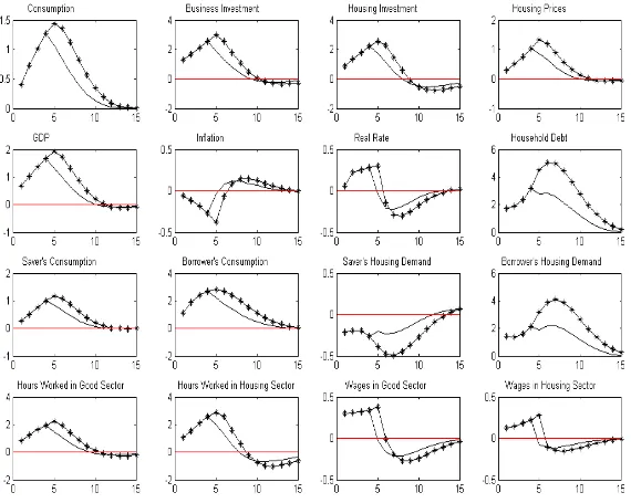
Expectations of future productivity gains generate boom-bust dynamics in GDP, consumption, hours, investment and house prices. See figure 15. The intuition is as follows. Expectations of higher productivity in the future lead households to increase their current consumption expenditure. Due to demand pressures, inflation increases. At the same time, the anticipation of higher productivity in the future generates expectations of higher future housing prices. The decline in the current real rate coupled with higher expected housing prices lead to an increase in Borrowers’ housing expenditure and indebtedness. Given the presence of limits to credit, impatient households increase their labor supply in order to raise internal funds for housing investment. Due to capital adjustment costs, firms already begin adjusting the stock of capital when news about a future reduction in the policy rate spread. For the increase in business investment to be coupled with an increase in total hours worked, wages must rise. The increase in business and housing investment makes GDP increase already at the time of the signal. A four-period anticipated increase in productivity generates a boom in housing prices, housing investment, consumption, GDP, hours and indebtedness. The peak response of all aggregate variables corresponds to the time in which expectations realize. After that all variables slowly return to their initial values. In contrast, if expectations do not realize there is a more substantial drop in both quantities and prices (solid line). See Appendix C for robustness analysis to different parameter values.
expectations on future productivity to generate co-movement between house prices and consump-tion, investment and hours worked. However, contrary to them, we obtain boom-bust dynamics in all aggregate variables and real wages. In our model house prices co-move with the other aggregate variables independently of whether wages are stickier than prices or vice versa. Intuitively, the increase in housing demand and therefore housing prices in response to news allows for an increase in both real wages and hours in the housing sector that spills over the consumption sector. The
empirical evidence in Figure 3 seems to suggest that real wages are not below trend before a peak
in house prices and that they increase throughout the boom phase. Notice also that the asset-price peak in the first quarter of the year 2000-2001 to which Christiano et al. (2008) refer to was pre-ceded by a rapid increase in real wages both in the consumption-good and in the housing sector –
see Figure 1.12
Figure 16 shows the effects of expectations of a future increase in the cost of transforming
out-put into capital,Ak. Agents are willing to increase their labor supply in order to reduce the future
negative effect of the shock. Consumption and housing expenditures increase. The increase in ag-gregate housing demand makes housing prices rise as well. Housing investment increases. Thus, the stock of capital used as input of production increases in both the consumption- and housing-good sector and total business investment goes up. As a result of the increase in the production of con-sumption goods, housing investment and business investment, GDP rises. Unrealized expectations induce a faster return to the initial state.
5.3.2 Supply and Demand in the Housing Market
Figure 17 shows that expectations of a future decline in productivity in the housing sector, a fall
inAh,t, makes agents increase their labor supply in order to reduce the future negative effect of the
shock. Moreover, news of negative housing supply shocks generate expectations of a future increase in house prices. To take advantage of lower current prices, Borrowers increase their current housing demand. Thus, both indebtedness and consumption expenditure increase. Due to adjustment
costs in capital, firms start adjusting the stock of capital already at the time of news.13 As
12In their model, the increase in hours is possible because the real wage falls, hence producers are willing to raise
labor demand. Since nominal wages are sticky, a decrease in real wages occurs because prices fall faster than wages.
The inflation-targeting central bank responds to this fall in inflation by cutting the nominal interest rate, which in
turn raises investment and the price of capital.
13The stock of capital (not shown in the graph) used as input of production in the consumption sector increases
a result, business investment slightly decreases on impact. Despite this, GDP rises due to the increase in housing investment and consumption. A four-period anticipated decline in productivity (starred line) generates a boom in housing prices, housing investment, consumption, GDP, hours and indebtedness. Still, current business investment slightly falls.
Figure 18 shows the response of the model economy to expectations of a future increase in
housing demand due to a housing preference shock, an increase inj. Anticipating a future increase
in housing prices, Borrowers raise their current demand for houses and thus indebtedness and consumption. Firms in the housing sector start adjusting their capital holding at the time of the signal and housing investment increases. Due to an expected shift in preference for housing relative to consumption, firms in the consumption sector reduce their stock of capital. As a result, business investment falls. Despite the decline in business investment, GDP rises. Because of the reduction in business investment during the boom phase, news about a future increase in housing demand fail to generate boom-bust dynamics consistent with the data. In the data business investment starts increasing already six periods before the peak in housing prices; in the model, however, it declines throughout the boom phase. Figure 19 considers the effect of an anticipated increase in
housing demand at different time horizons: n = {4,6,8}. Expectations of a change in housing
demand further in the future only postpone the occurrence of the peak. The behavior of business investment is independent of the time horizon of the expected increase in housing demand. The decline in business investment is also robust to different parametrization of key model’s parameters. See Appendix C.
6
Credit Market and Housing Market Fluctuations
Are economies characterized by lower lending standards more vulnerable to boom-bust cycles in the housing market? We analyze how credit market conditions affect the steady state of the model, the transmission of news shocks and the implied volatility. We borrow from previous literature the
notion that the collateral requirement, m, can serve as proxy for credit market development.14 To
be precise, tighter collateral constraints (lower values ofm) result in a smaller size of the mortgage
market and thereby characterize economies with a higher degree of frictions in the credit market.
14See, among others, Aghion et al. (2003), Campbell and Hercowitz (2005), Mendicino (2007), Calza, Monacelli
6.1 Long-run Effects
Figure 20 shows that increased access to the credit market, namely a higher value of m, implies a
credit expansion in the steady state and thus larger housing investment by Borrowers. In contrast,
Borrowers’ consumption decreases with an increase in m. An environment with a lower degree of
credit frictions allows impatient agents to consume more in the present than in the future. Hence their steady-state consumption level is lower. On the contrary, Savers are better able to postpone consumption, thereby raising their steady-state consumption level. Total consumption as well as
business and residential investment increase at the steady state with higher values ofm. Increased
housing demand leads to higher housing prices that further contribute to higher indebtedness. A reduced level of consumption for Borrowers is coupled with higher labor supply. Despite the decline
in hours for Savers, overall labor supply and GDP increase withm. To sum up, a lower degree of
credit frictions characterizes economies with higher levels of indebtedness, investment, production and consumption.
6.2 Transmission Mechanism
To document the role of the degree of credit frictions for the transmission of expectations-driven business cycles, we consider the case of expectations of a future lower policy interest rate. Figure 21
compares the transmission of news shocks in the case of the benchmark loan-to-value ratio (m=0.85)
with a lower (m=0.20) and a higher (m =0.95) value. Consumption, GDP and indebtedness are
quite sensitive to the degree of credit frictions and they show more pronounced booms and busts
as the value ofm increases. On the other hand, the responses of the other aggregate variables are
barely affected. The degree of credit frictions plays an important role at the individual level. In particular, the response of Borrower’s consumption and housing demand to the news shock and to its missing realization are magnified by lower credit constraints.
short run Savers raise their consumption but reduce their holding of houses. The contemporaneous positive response for consumption and negative one for housing demand become more polarized as
m gets bigger and closer to one. Intuitively, this is a rational response to the increase of housing
prices during the boom phase. Moreover, substituting housing with consumption makes Savers able to maintain a similar increase in consumption independently of the degree of credit frictions. As a result, total consumption displays larger contemporaneous and boom responses with higher values
of m, as shown in Figures 21 and 22.
Borrower’s consumption and housing investment display deeper troughs and more sizable cu-mulated busts in more developed credit markets. In economies with a low degree of credit frictions Borrowers are more leveraged. When expectations do not materialize, the drop in Borrowers’ con-sumption expenditure is more sizable, which in turn makes aggregate concon-sumption more responsive to unrealized expectations - see Figure 23. In contrast, housing prices, business and residential
investment display cumulated booms and busts of smaller magnitude as m gets bigger. Similar
results hold for the case of a change in expectations about future productivity, as shown in Figure 23.
6.3 Volatility
Figures 24 show how the degree of credit market development affects macroeconomic volatility in the presence of news shocks. The volatilities of consumption, household debt and hours worked in
the consumption sector increase with an increase m. In contrast, the volatilities of housing prices,
housing investment and business investment decline. The volatility of aggregate housing investment declines despite the increase in the volatility of individual investment. Aggregate housing invest-ment becomes less volatile because the correlation between housing investinvest-ment by the two types of agents falls. As shown in Figure 24, housing demand by Borrowers and Savers move in oppositive directions in response to news on monetary policy and the difference grows larger as the degree of credit frictions falls. Accordingly, the volatility of hours worked increases in the consumption-good
sector while it decreases in the housing sector asm rises.
– see Figure 25.15 The sensitivity of the other variables to the degree of credit frictions is not affected by the way we measure GDP. Movements in relative prices play an important role in the
transmission of shocks to GDP.16
7
Conclusions
We study the role of expectations-driven fluctuations in generating boom-bust cycle dynamics in the housing market. First, we document that the cyclical behavior of housing prices and housing investment is coupled with a similar pattern in GDP, business investment, consumption, hours worked and real wages. Then we show that expectations about the future state of productivity, investment cost, housing supply, inflation, the policy rate and the central bank’s target can generate housing-market booms in accordance with the empirical findings. However, only expectations of either a future reduction in the policy rate or a temporary increase in the central bank’s inflation target that are not fulfilled can generate macroeconomic recessions. Thus, good communication on monetary policy is essential for reducing the occurrence of expectations-driven cycles.
Regarding the role of the credit market in housing market fluctuations, we document that easier access to credit can generate boom-bust cycles dynamics only if agents expect current favorable credit conditions to be reversed in the near future. We also show that more developed credit markets are characterized by higher sensitivity of consumption and household indebtedness to changes in expectations. However, if the measurement of GDP allows for variable relative prices, more developed credit markets may experience lower volatility of real GDP.
A quantitative assessment of the relative importance of each shock in generating boom-bust cycles through estimation requires separate consideration. The role of monetary policy, as well as the analysis of the optimal conduct of monetary policy, is also left to future research.
15In recent years, an increasing number of countries have changed from the constant price measure of GDP to the
chain volume measure of GDP that takes into account movements in relative prices. See among others the United
States, Canada, Australia, New Zealand, Japan, UK, Hong Kong and most European economies.
16This result is in accordance with Mendicino (2007). The author, using a real business cycle model in which
entrepreneurs borrow in order to partly finance their investment in capital, highlights the key role of the relative
References
[1] Aghion, P., Philippe B. and A. Banerjee. 2003. “Financial Development and the Instability of
Open Economies,”Journal of Monetary Economics,1077-1106.
[2] Ahearne, A.G., J. Ammer, B.M. Doyle, L.S. Kole and R.F. Martin. 2005. “House Prices and Monetary Policy: A Cross-Country Study,” Board of Governors of the Federal Reserve System International Finance Discussion Papers 841.
[3] Arce, O. and J. D. Lopez-Salido. 2008. “Housing Bubbles,” forthcoming in the American
Economic Journal: Macroeconomics.
[4] Barsky, R. B. and E. R. Sims. 2009. “News Shocks,” mimeo.
[5] Basant Roi, M. and R. Mendes. 2007. “Should Central Banks Adjust Their Target Horizons in Response to House-Price Bubbles?” Bank of Canada Discussion Papers 07-4.
[6] Beaudry, P. and F. Portier. 2004. “An Exploration into Pigou’s Theory of Cycles,” Journal of
Monetary Economics,51: 1183-1216.
[7] Beaudry, P. and F. Portier. 2006. “Stock Prices, News, and Economic Fluctuations,”American
Economic Review,96(4): 1293-1307.
[8] Beaudry, P. and F. Portier. 2007. “When can Changes in Expectations Cause Business Cycle
Fluctuations in Neo-classical Settings?” Journal of Economic Theory,135(1): 458-477.
[9] Bernanke B. and M. Gertler. 1999. “Monetary Policy and Asset Price Volatility,” In New Challenges for Monetary Policy, 77-128, Federal Reserve Bank of Kansas City.
[10] Borio C. and P. Lowe. 2002. “Asset Prices, Financial and Monetary Stability: Exploring the Nexus,” BIS Working Paper 114.
[11] Campbell, J. 1994. “Inspecting the Mechanism: an Analytical Approach to the Stochastic
Growth Model,”Journal of Monetary Economics, 33(3): 463-506.
[13] Christiano, L., C. Ilut, R. Motto and M. Rostagno. 2008. “Monetary Policy and Stock Market Boom-Bust Cycles,” ECB Working Paper 955.
[14] Den Haan, W.J. and G. Kaltenbrunner. 2007. “Anticipated Growth and Business Cycles in Matching models,” CEPR Discussion Paper 6063.
[15] Floden, M. 2007. “Vintage Capital and Expectations Driven Business Cycles,” CEPR Discus-sion Paper 6113.
[16] Greenwood, J., G. W. Huffman and Z. Hercowitz. 1988. “Investment, Capacity Utilization,
and the Real Business Cycle,”American Economic Review,78(3): 402-17.
[17] Horvath, M. 2000. “Sectoral Shocks and Aggregate Fluctuations,” Journal of Monetary
Eco-nomics,45(1): 69-106.
[18] Iacoviello, M. 2005. “House Prices, Borrowing Constraints, and Monetary Policy in the
Busi-ness Cycle,”American Economic Review,95(3): 739-64.
[19] Iacoviello, M. and S. Neri, 2009. “Housing Market Spillovers: Evidence from an Estimated
DSGE Model.” forthcoming inAmerican Economic Journal: Macroeconomics.
[20] Jaimovich, N. and S. Rebelo. 2009. “Can News about the Future Drive the Business Cycle?”
forthcoming inAmerican Economic Review.
[21] Kengo, N. 2009. “Internal and External Habits and News-Driven Business Cycles,” MPRA.
[22] Khan, H. and J. Tsoukalas. 2009. “The Quantitative Importance of News Shocks in Estimated DSGE Models,” mimeo.
[23] Kiyotaki, N. and J. Moore. 1997. “Credit Cycles,”Journal of Political Economy,105(2):
211-48.
[24] Kobayashi, K., T. Nakajima and M. Inaba. 2007. “Collateral Constraint and News-driven Cycles,” Discussion paper 07013, Research Institute of Economy, Trade and Industry (RIETI).
[25] Kurmann, A. and C. Otrok. 2010. “News Shocks and the Slope of the Terms Strucure of Interest Rates,” mimeo.
[27] Monacelli, T. 2009. “New Keynesian Models, Durable Goods, and Collateral Constraints,”
Journal of Monetary Economics 56(2): 242-54.
[28] Schmitt-Grohe, S. and M. Uribe. 2008. “What’s News in Business Cycles,” NBER Working Paper No. 14215.
[29] Walentin, K. 2009. “Expectation Driven Business Cycles with Limited Enforcement,” Working Paper Series 229, Sveriges Riksbank.
[30] Wouters, R. and F. Smets. 2003. “Output Gaps: Theory versus Practice,” Computing in
Appendix
A
DataCC : Aggregate Consumption. Real Personal Consumption Expenditure (seasonally adjusted,
billions of chained 2005 dollars, Table 1.1.6), divided by the Civilian Noninstitutional Popu-lation (CNP16OV, source: Bureau of Labor Statistics). Source: Bureau of Economic Analysis (BEA).
GDP : Gross Domestic Product. Real Gross Domestic Product (seasonally adjusted, billions of
chained 2005 dollars, Table 1.1.6), divided by CNP16OV. Source: BEA.
IK : Business Fixed Investment. Real Private Nonresidential Fixed Investment (seasonally
ad-justed, billions of chained 2005 dollars, Table 1.1.6), divided by CNP16OV. Source: BEA.
IH : Residential Investment. Real Private Residential Fixed Investment (seasonally adjusted,
billions of chained 2005 dollars, Table 1.1.6.), divided by CNP16OV. Source: BEA.
INFLQ : Inflation. Quarter on quarter log differences in the implicit price deflator for the nonfarm business sector, demeaned. Source: Bureau of Labor Statistics (BLS).
RRQ : Real Short-term Interest Rate. 3-month Treasury Bill Rate (Secondary Market Rate),
expressed in quarterly units, minus quarter on quarter log difference in the implicit price deflator for the nonfarm business sector; demeaned. (Series ID: H15/RIFSGFSM03 NM). Source: Board of Governors of the Federal Reserve System.
QQ : Real House Prices. Census Bureau House Price Index (new one-family houses sold including
value of lot) deflated with the implicit price deflator for the nonfarm business sector. Source: Census Bureau, http://www.census.gov/const/price sold cust.xls.
NC : Hours in Consumption Sector. Total Nonfarm Payrolls (Series ID: PAYEMS in Saint Louis
Fed Fred2) less all employees in the construction sector (Series ID: USCONS), times Average Weekly Hours of Production Workers (series ID: CES0500000007), divided by CNP160V. Source: BLS.
NH : Hours in Housing Sector. All Employees in the Construction Sector (Series ID: USCONS
RWCPC : Real Wage in Consumption-good Sector. Average Hourly Earnings of Production/ Nonsupervisory Workers on Private Nonfarm Payrolls, Total Private (Series ID: CES0500000008), divided by the price index for Personal Consumption Expenditure (Table 2.3.4, source: BEA). Source: BLS.
RWHPC : Real Wage in Housing Sector. Average Hourly Earnings of Production/Nonsupervisory Workers in the Construction Industry (Series ID: CES2000000008), divided by the price index for Personal Consumption Expenditure (Table 2.3.4, source: BEA). Source: BLS.
RLOANS : Households and nonprofit organizations home mortgages liability (seasonally ad-justed, millions of current dollars), divided by the implicit price deflator and divided by the Civilian Noninstitutional Population. Source: The Federal Reserve Board (Series ID: Z1/Z1/LA153165105.Q).
B
Housing Prices Peaks: 1965:1-2009:2
C
Sensitivity Analysis
The results presented in Sections 4 and 5 are robust to different parametrization of the labor share
income of credit-constrained agents, α, the loan-to-value ratio, m, the capacity utilization rate,
zc,t, and the labor mobility across sectors,ξ andξ
′
D
Expectations about Future Productivity
The model presented above features several real and nominal rigidities. In order to disentangle the contribution of the different modeling choices, we introduce the frictions one at the time. Figure 30 displays the boom-bust response to news on productivity in the flexible-price version of the model. In the absence of adjustment costs of capital and when impatient households cannot borrow
(dashed line), i.e. whenm= 0, the wealth effect dominates and agents increase both consumption
and leisure. To increase consumption households reduce their investment expenditures (in all sectors). When it is costly to adjust the stock of capital, the reduction in business investment and thus the increase in consumption is less pronounced (starred line). Allowing for borrowing against the value of collateral leads to a more pronounced increase in Borrower’s housing demand (solid line). In this last case, Borrower’s consumption increases by more in the boom phase and the decline in Borrower’s hours (not shown in the graph) is more sizable. Saver’s demand for housing declines. Since Savers account for about eighty percent of labor income, aggregate housing production declines and housing prices fall. To sum up, adjustment costs and the collateral effect are not enough to generate boom-bust dynamics in the absence of nominal rigidities.
Figures 31 shows the response of the economy with nominal rigidity in the price of the con-sumption good but no wage rigidities (dashed line). Expectations of higher future productivity lead to a decrease in expected inflation, which in turn reduces the expected real interest rate. The decline in the current real interest rate coupled with a higher expected real rate lead to an in-crease in current debt and thus Borrowers’ consumption, Borrowers’ housing demand and Savers’ consumption. On the contrary, Savers reduce their housing demand and increase their supply of labor. For a contemporaneous increase in business investment and hours, the rise in wages in the consumption sector needs to be significant. Aggregate housing investment first declines and then slowly increases; housing prices increase as well as current inflation. However, compared to the case with flexible prices, inflation rises by less, thereby allowing for a more pronounced increase in consumption.
E
Tables and FiguresCorrelation with QQHP
1965:1 to 2009:2 Boom-Bust Episodes
GDPHP 0.60 0.64
CCHP 0.54 0.60
IKHP 0.55 0.58
IHHP 0.49 0.53
RLOANSHP 0.76 0.84
NCHP 0.62 0.62
NHHP 0.71 0.71
RRQHP 0.11 0.09
INFLQHP 0.29 0.23 RWCPCHP 0.20 0.31
RWHPCHP -0.10 0
Standard Deviation
GDPHP 1.56 1.65
CCHP 1.85 2.13
IKHP 5.08 4.83
IHHP 10.23 12.41
RLOANSHP 2.46 2.47
NCHP 1.69 1.76
NHHP 4.38 4.60
RRQHP 0.38 0.48
INFLQHP 0.40 0.51 RWCPCHP 0.99 1.32 RWHPCHP 1.15 1.42
[image:33.612.177.432.114.594.2]QQHP 2.23 2.31
Table 1: Descriptive Statistics for H-P filtered data: Full Sample and Boom-Bust Episodes.
0.0 0.2 0.4 0.6 0.8 1.0
65 70 75 80 85 90 95 00 05
Real Consumption .0 .2 .4 .6 .8
65 70 75 80 85 90 95 00 05
Real GDP 0.00 0.25 0.50 0.75 1.00 1.25 1.50
65 70 75 80 85 90 95 00 05
Real Business Investment
-.6 -.4 -.2 .0 .2 .4 .6
65 70 75 80 85 90 95 00 05
Real Residential Investment
0.0 0.4 0.8 1.2 1.6 2.0
65 70 75 80 85 90 95 00 05
Real Loans -.2 .0 .2 .4 .6 .8
65 70 75 80 85 90 95 00 05
Real House Prices
.00 .05 .10 .15 .20 .25 .30
65 70 75 80 85 90 95 00 05
Hours Worked, Consumption Sector
-.2 -.1 .0 .1 .2 .3
65 70 75 80 85 90 95 00 05
Hours Worked, Housing Sector
.0 .1 .2 .3 .4
65 70 75 80 85 90 95 00 05
Real Wage, Consumption Sector
.0 .1 .2 .3 .4
65 70 75 80 85 90 95 00 05
Real Wage, Housing Sector
-.02 -.01 .00 .01 .02 .03
65 70 75 80 85 90 95 00 05
Inflation -.03 -.02 -.01 .00 .01 .02
65 70 75 80 85 90 95 00 05
[image:34.612.65.728.139.510.2]Real Interest Rate
Figure 1: Macroeconomic Variables in the United States, 1965:1 to 2009:2
.28 .30 .32 .34 .36 .38 .40
2 4 6 8 10 12 14 16 18 20
Real House Prices
.39 .40 .41 .42 .43 .44 .45
2 4 6 8 10 12 14 16 18 20
Real Consumption .32 .34 .36 .38 .40
2 4 6 8 10 12 14 16 18 20
Real GDP .56 .60 .64 .68 .72 .76
2 4 6 8 10 12 14 16 18 20
Real Business Investment
-.2 -.1 .0 .1 .2 .3
2 4 6 8 10 12 14 16 18 20
Real Residential Investment
.56 .60 .64 .68 .72 .76
2 4 6 8 10 12 14 16 18 20
Real Loans .11 .12 .13 .14 .15 .16
2 4 6 8 10 12 14 16 18 20
Hours Worked, Consumption Sector
-.05 .00 .05 .10 .15
2 4 6 8 10 12 14 16 18 20
Hours Worked, Housing Sector
.175 .180 .185 .190 .195 .200
2 4 6 8 10 12 14 16 18 20
Real Wage, Consumption Sector
.260 .264 .268 .272 .276 .280
2 4 6 8 10 12 14 16 18 20
Real Wage, Housing Sector
-.006 -.004 -.002 .000 .002 .004
2 4 6 8 10 12 14 16 18 20
Real Interest Rate
-.004 .000 .004 .008 .012
2 4 6 8 10 12 14 16 18 20
[image:35.612.59.556.25.333.2]Inflation
Figure 2: Macroeconomic Variables during Peaks: Average over all Peaks
-.04 -.02 .00 .02 .04 .06
2 4 6 8 10 12 14 16 18 20
Real House Prices
-.04 -.02 .00 .02 .04
2 4 6 8 10 12 14 16 18 20
Real Consumption -.02 -.01 .00 .01 .02 .03
2 4 6 8 10 12 14 16 18 20
Real GDP -.06 -.04 -.02 .00 .02 .04 .06 .08
2 4 6 8 10 12 14 16 18 20
Real Business Investment
-.2 -.1 .0 .1 .2
2 4 6 8 10 12 14 16 18 20
Real Residential Investment
-.04 -.02 .00 .02 .04
2 4 6 8 10 12 14 16 18 20
Real Loans -.02 -.01 .00 .01 .02 .03
2 4 6 8 10 12 14 16 18 20
Hours Worked, Consumption Sector
-.08 -.04 .00 .04 .08
2 4 6 8 10 12 14 16 18 20
Hours Worked, Housing Sector
-.010 -.005 .000 .005 .010
2 4 6 8 10 12 14 16 18 20
Real Wage, Consumption Sector
-.012 -.008 -.004 .000 .004 .008
2 4 6 8 10 12 14 16 18 20
Real Wage, Housing Sector
-.006 -.004 -.002 .000 .002 .004 .006
2 4 6 8 10 12 14 16 18 20
Real Interest Rate
-.004 -.002 .000 .002 .004
2 4 6 8 10 12 14 16 18 20
Inflation
[image:35.612.61.555.366.674.2]