Discrete adjoint based simultaneous analysis and design approach for conceptual aerodynamic optimization

Discrete adjoint­based simultaneous 

analysis and design approach for 

conceptual aerodynamic optimization

Sugar­Gabor, O

10.13111/2066­8201.2017.9.3.11

Title

Discrete adjoint­based simultaneous analysis and design approach for 

conceptual aerodynamic optimization

Authors

Sugar­Gabor, O

Type

Article

URL

This version is available at: http://usir.salford.ac.uk/id/eprint/43738/

Published Date

2017

USIR is a digital collection of the research output of the University of Salford. Where copyright 

permits, full text material held in the repository is made freely available online and can be read, 

downloaded and copied for non­commercial private study or research purposes. Please check the 

manuscript for any further copyright restrictions.

Approach for Conceptual Aerodynamic Optimization

Oliviu SUGAR-GABOR*

*Corresponding author

Department of Aeronautical and Mechanical Engineering, School of Computing,

Science and Engineering, University of Salford,

The Crescent, M5 4WT, Salford, United Kingdom,

[email protected]

DOI: 10.13111/2066-8201.2017.9.3.11

Received:13 July 2017/ Accepted: 18 August 2017/ Published: September 2017

Copyright©2017. Published by INCAS. This is an “open access” article under the CC BY-NC-ND license (http://creativecommons.org/licenses/by-nc-nd/4.0/)

Abstract: In this paper, a simultaneous analysis and design method is derived and applied for a non-linear constrained aerodynamic optimization problem. The method is based on the approach of defining a Lagrange functional based on the objective function and the aerodynamic model’s equations, using two sets of multipliers. A fully-coupled, non-linear system of equations is derived by requiring that the Gateaux variation of the Lagrange functional vanishes for arbitrary variations of the aerodynamic model’s dependent variables and design parameters. The optimization problem is approached using a one-shot technique, by solving the non-linear system in which all sensitivities and problem constraints are included. The computational efficiency of the method is compared against a gradient-based optimization algorithm using adjoint-provided gradient. A conceptual-stage aerodynamic optimization problem is solved, based on a non-linear numerical lifting-line method with viscous corrections.

Key Words: Simultaneous Analysis and Design, Adjoint-Based Optimization, Discrete Adjoint, Aerodynamic Optimization, Non-linear Lifting-Line Method

1. INTRODUCTION



Aerodynamic optimization represents a discipline at the crossroads of several scientific and research areas such as geometry modelling, aerodynamic simulation, applied mathematics, non-linear optimization and computer science [1]. Because the use of high-fidelity CFD simulations in the aerodynamic design of aircraft has been steadily and rapidly increasing, the application of various optimization algorithms has been attempted, in an attempt to minimize the required number of CFD solutions and to increase the computational efficiency of the design and optimization process.

Using the adjoint method, each design iteration requires one flow equations solution and one adjoint equations solution. This represents a very significant advantage over the finite-differences approach, where a number of flow equations solutions equal to the number of design variables is required to determine the objective function gradient. The optimization process and the values of the design variables are driven by a gradient-based constrained optimization algorithm, such as the Method of Feasible Directions (MFD), Sequential Quadratic Programming (SQP) or the penalty function augmented Broyden-Fletcher-Goldfarb-Shanno (BFGS) [4].

The implementation of the adjoint method in aerodynamic optimization using the Euler or Navier-Stokes equations has been carried out using two approaches: continuous adjoint and discrete adjoint [5]. In the first approach, the adjoint equations are deduced from the continuous form of the flow equations, and thus are also nonlinear partial-differential equations, requiring an appropriate set of boundary conditions. In the second approach, the adjoint equations are determined from the spatially and temporally-discretized flow equations, and thus will represent a linear system of equations, with any boundary conditions already included in the linear system terms.

Aerodynamic optimization using gradient-based optimization algorithms coupled with and adjoint-equation gradient computation have been extensively used over the last years, for a wide variety of problems across various industries. These include helicopter rotors [6], automobiles [7], wide-body transport aircraft [8] supersonic aircraft configurations [9], tidal turbines [10] and ship hulls [11].

Even with the increase in popularity of the adjoint approach, driven by the significant reduction in computational effort it provides, other algorithms such as non-deterministic global optimization algorithm are still commonly used in aerodynamic optimization problems, despite their relatively high computational costs. Similarly to the adjoint-method optimization, these algorithms have been applied to solve problems in a wide range of engineering applications. More recently, genetic algorithms (GA) have been used for wind turbine blades [12], for the shape optimization of a morphing wing wind tunnel technical demonstrator [13], [14], while the artificial bee colony (ABC) algorithm has been used for the numerical analysis of a UAV morphing wing [15]. A significant advantage of gradient-free global optimization algorithms is that they can be very easily configured to run on massively-parallel computers in order to reduce the overall execution time.

The present paper presents a methodology for further reducing the computational cost of the discrete adjoint method, with the construction of an adjoint-based simultaneous analysis and design technique. A Lagrange functional is defined based on the objective function and the aerodynamic model’s equations, and by using two sets of Lagrange multipliers (which also represent the adjoint variables) [16], [17]. By imposing the requirement that the Gateaux variation of Lagrange functional vanish for arbitrary variations of the system dependent variables and design parameters, a set on non-linear equations is determined. The optimization problem of minimizing the objective function is then solved simultaneously with the aerodynamic model’s equations, by using the one-shot approach, as the solution of the constructed non-linear system (which takes into consideration all sensitivities and imposed constraints).

2. MATHEMATICAL MODEL

stages of aircraft conceptual design, the problem reduces to solving a system of algebraic equations. Let the algebraic system of linear or non-linear equations be:

𝑹(𝒘, 𝜶) = 𝟎, 𝑹: ℝ𝑁_{× ℝ}𝐷_{→ ℝ}𝑁 ₍₁₎

where 𝒘 ∈ ℝ𝑁 are the system dependent variables and 𝜶 ∈ ℝ𝐷 are the system design

parameters, whose values must be given in order to determine a solution for the system of equations.

The aerodynamic characteristics of aerofoil and wings, such as the lift and drag coefficients, the chord-wise pressure distribution or the span-wise lift distribution, are functions of both dependent variables and system parameters. The objective function to be minimised is given by:

𝐽(𝒘, 𝜶), 𝐽: ℝ𝑁_{× ℝ}𝐷_{→ ℝ (2)}

When searching to minimise a given objective function with respect to the design parameters, the problem usually includes equality and/or inequality constraints, as well as upper and lower bounds imposed on the design parameters in order to limit their variation to some feasible design space. Let all such constraints be given by:

𝑮(𝒘, 𝜶) ≤ 𝟎, 𝑮: ℝ𝑁_{× ℝ}𝐷_{→ ℝ}𝐾 ₍₃₎

In order to minimize the objective function (2), subject to the equality and inequality constraints given by (3) and to satisfying the system of equations (1) that models the aerodynamic problem, a Lagrange functional can be defined [16]:

𝐿(𝒘, 𝝍_𝟏, 𝜶, 𝝍_𝟐) = 𝐽(𝒘, 𝜶) + (𝝍𝟏, 𝑹(𝒘, 𝜶))𝑁+ (𝝍𝟐, 𝑮(𝒘, 𝜶))𝐾 (4)

where 𝝍_𝟏∈ ℝ𝑁 and 𝝍_𝟐∈ ℝ𝐾 are two sets of Lagrange multipliers, which will also play the

role of the adjoint variables.

The critical points of the objective function 𝐽 will be among the points that cause the

Gateaux variation 𝛿𝐿 of the Lagrange functional (4) to become zero for arbitrary variations

of the independent variables, design variables and Lagrange multipliers. The Gateaux variation of (4) is given by:

𝛿𝐿 = 𝑑

𝑑𝜀[𝐽 + 𝜀𝛿𝐽 + (𝝍𝟏+ 𝜀𝜹𝝍𝟏, 𝑹 + 𝜀𝜹𝑹)𝑁+ (𝝍𝟐+ 𝜀𝜹𝝍𝟐, 𝑮 + 𝜀𝜹𝑮)𝐾]|_𝜀=0 (5)

In addition, the following equations can be written:

𝛿𝐽(𝒘, 𝜶) =𝜕𝐽

𝑇

𝜕𝒘𝜹𝒘 + 𝜕𝐽𝑇

𝜕𝜶𝜹𝜶, 𝜹𝑹(𝒘, 𝜶) = 𝜕𝑹 𝜕𝒘𝜹𝒘 +

𝜕𝑹 𝜕𝜶𝜹𝜶, 𝜹𝑮(𝒘, 𝜶) = 𝜕𝑮

𝜕𝒘𝜹𝒘 + 𝜕𝑮 𝜕𝜶𝜹𝜶

(6)

All the derivatives appearing in the gradient vectors and Jacobian matrices of (6) are Gateaux partial derivatives.

Introducing (6) into (5), and using the linear properties of the inner product, the Gateaux variation of the Lagrange functional is given by:

𝛿𝐿 = (𝜕𝐽

𝜕𝒘, 𝜹𝒘)_𝑁+ ( 𝜕𝐽

𝜕𝜶, 𝜹𝜶)_𝐾+ (𝝍𝟏, 𝜕𝑹

𝜕𝒘𝜹𝒘)_𝑁+ (𝝍𝟏, 𝜕𝑹

𝜕𝜶𝜹𝜶)_𝑁+ +(𝑹, 𝜹𝝍𝟏)𝑁+ (𝝍𝟐,

𝜕𝑮

𝜕𝒘𝜹𝒘)𝐾+ (𝝍𝟐,

𝜕𝑮

𝜕𝜶𝜹𝜶)𝐾+ (𝑮, 𝜹𝝍𝟐)𝐾

In the n-dimensional real space ℝ𝑛, a linear operator 𝐿+ is the adjoint to the operator 𝐿 if

the following equation can be written for any two vectors 𝒙, 𝒚 ∈ ℝ𝑛, where ( , ) denotes the

inner product:

(𝐿𝒙, 𝒚) = (𝒙, 𝐿+_{𝒚) (8)}

Using the above defined property of adjoint operators, the Jacobian matrices appearing in (7) can be transferred to the Lagrange multipliers and replaced with their corresponding adjoint:

𝛿𝐿 = (_𝜕𝒘𝜕𝐽 +𝜕𝑹 𝜕𝒘

+

𝝍_𝟏+𝜕𝑮 𝜕𝒘

+

𝝍_𝟐, 𝜹𝒘)

𝑁

+ (𝑹, 𝜹𝝍_𝟏)_𝑁+

+ (𝜕𝐽 𝜕𝜶+

𝜕𝑹 𝜕𝜶

+

𝝍_𝟏+𝜕𝑮 𝜕𝜶

+

𝝍_𝟐, 𝜹𝜶)

𝐾

+ (𝑮, 𝜹𝝍_𝟐)_𝐾

(9)

Requiring that the Gateaux variation 𝛿𝐿 of the Lagrange functional becomes zero for arbitrary variations of the independent variables, design variables and Lagrange multipliers leads to the following set of equations:

𝜕𝐽 𝜕𝒘+

𝜕𝑹 𝜕𝒘

+

𝝍_𝟏+𝜕𝑮 𝜕𝒘

+

𝝍_𝟐 = 𝟎 (10)

𝑹 = 𝟎 (11)

𝜕𝐽

𝜕𝜶+

𝜕𝑹 𝜕𝜶

+

𝝍𝟏+

𝜕𝑮 𝜕𝜶

+

𝝍𝟐= 𝟎 (12)

(𝑮, 𝜹𝝍𝟐)𝐾= 0 (13)

The first equation represents the typical adjoint equation found in literature, with an extra term given by the product between the constraints sensitivities to the dependent variables and the second adjoint vector. The second equation is the system of linear or non-linear algebraic equations that defines the aerodynamic model. The third equation contains all the sensitivities with respect to the design variables. The fourth equation is replaced with the equivalent form, following the methodology proposed in [16], [17]:

𝐶𝑖= (𝐺𝑖+ 𝜓2𝑖)

2

+ 𝐺𝑖|𝐺𝑖| + 𝜓2𝑖|𝜓2𝑖|, 𝑖 = 1, 𝐾̅̅̅̅̅ (14)

Using the equivalence introduced in (14), the set of equations presented in (10) to (13) can be written as a coupled non-linear system:

𝑭 = [ 𝜕𝐽 𝜕𝒘+ 𝜕𝑹 𝜕𝒘 +

𝝍_𝟏+𝜕𝑮 𝜕𝒘 + 𝝍_𝟐 𝑹 𝜕𝐽 𝜕𝜶+ 𝜕𝑹 𝜕𝜶 +

𝝍_𝟏+𝜕𝑮 𝜕𝜶

+

𝝍_𝟐

𝑪 ]

= 𝟎, 𝑭: ℝ𝑁_{× ℝ}𝑁_{× ℝ}𝐷_{× ℝ}𝐾_{→ ℝ}𝑁+𝑁+𝐷+𝐾 ₍₁₅₎

The solution of the above system, (𝒘, 𝝍𝟏, 𝜶, 𝝍𝟐)𝑇, includes the optimal values of the

design parameters as required to minimise the objective function 𝐽, the solution of the system

parameters, and the values for the two vectors of adjoint variables. In order to obtain the solution of the non-linear system of equations presented in (15), the trust-region method is used [18]. The choice is justified by the fact that numerical tests have shown that the Jacobian matrix of the system may become ill-conditioned or even singular at some points. In the trust-region method, the solution is updated iteratively, starting from an initial guess:

𝒙_𝑘+1= 𝒙_𝑘+ ∆𝒙 (16)

At each iteration, the solution step is constructed from a convex combination of a Cauchy step, along the steepest descent direction, and a Newton step. The Cauchy step is determined as:

∆𝒙𝐶 = −𝛽𝑱(𝒙𝑘)𝑻𝑭(𝒙𝑘) (17)

Where the step 𝛽 is chosen to minimise the trust-region sub-problem, using Powell’s efficient dogleg procedure [19]:

min

∆𝒙𝐶 [

1

2𝑭(𝒙𝑘)𝑻𝑭(𝒙𝑘) + ∆𝒙𝐶𝑻𝑱(𝒙𝑘)𝑻𝑭(𝒙𝑘) + 𝟏

𝟐∆𝒙𝐶𝑻𝑱(𝒙𝑘)𝑻𝑱(𝒙𝑘)∆𝒙𝐶] (18)

The Newton step is calculated by solving the linearized system of equations:

𝑱(𝒙_𝑘)∆𝒙𝑁 = −𝑭(𝒙𝑘) (19)

The step used to update the solution is then computed as a combination between the

Cauchy and Newton steps, where 𝜆 is a parameter in the interval [0,1]:

∆𝒙 = ∆𝒙𝐶+ 𝜆(∆𝒙𝑁− ∆𝒙𝐶) (20)

If the Jacobian matrix is ill-conditioned or singular, then the step is taken only along the Cauchy direction. The trust-region method is computationally efficient, since it requires only one linear system solution per iteration, for the computation of the Newton step, while the Cauchy step requires only matrix-matrix and matrix-vector multiplications, which are computationally inexpensive using vectorised algorithms (such as implemented in the MATLAB software package).

3. CLASSICAL ADJOIT APPROACH

Constructing the adjoint equation in order to eliminate the dependency of the objective function gradient on the flow-field variables, and then using advanced gradient-based optimisation algorithms is today one the most popular approaches to performing aerodynamic design and optimisation.

The objective function is the one defined in (2), and any variations in the design parameters values cause variations in both the objective function and the system of equations governing the aerodynamic problem:

𝛿𝐽(𝒘, 𝜶) =𝜕𝐽𝑇 𝜕𝒘𝜹𝒘 +

𝜕𝐽𝑇

𝜕𝜶 𝜹𝜶

𝜹𝑹(𝒘, 𝜶) =𝜕𝑹 𝜕𝒘𝜹𝒘 +

𝜕𝑹 𝜕𝜶𝜹𝜶

(21)

It must be kept in mind that the governing equations defined in (1) are solved at each

can be multiplied by a Lagrange multiplier and subtracted from the variation 𝛿𝐽 without changing the result:

𝜹𝑱(𝒘, 𝜶) = [𝜕𝐽𝑇 𝜕𝒘− 𝝍𝑻

𝜕𝑹

𝜕𝒘] 𝜹𝒘 + [ 𝜕𝐽𝑇

𝜕𝜶 − 𝝍𝑻 𝜕𝑹

𝜕𝜶] 𝜹𝜶 (22)

If the first term of the objective function variation could be set to zero, then the gradient would be independent of the variations of the dependent variables (flow variables) caused by

the design parameters variations. Thus, by choosing 𝝍 to satisfy the adjoint equation:

𝜕𝑹 𝜕𝒘

𝑇

𝝍 = 𝜕𝐽

𝜕𝒘 (23)

The first term is eliminated, and (22) is written as:

𝛿𝐽(𝒘, 𝜶) = [𝜕𝐽

𝑇

𝜕𝜶 − 𝝍𝑻 𝜕𝑹

𝜕𝜶] 𝜹𝜶 = 𝓖𝜹𝜶 (24)

The interior point optimisation algorithm also requires the gradient, with respect to the design variables, of any non-linear equality or inequality constraints (such as the one presented in (3)). In order to preserve the computational efficiency of the adjoint method, the constraints that depend on the system dependent variables (flow-field variables) are traditionally not treated as independent functions, but instead are added as a series of penalty terms to the objective function [20]:

𝐽(𝒘, 𝜶) → 𝐽(𝒘, 𝜶) + 𝜆₁𝐺₁(𝒘, 𝜶) + 𝜆2𝐺2(𝒘, 𝜶) + ⋯ (25)

This way, the adjoint equation (23) and the gradient defined in (24) must be modified as follows in order to include the constraint:

𝜕𝑹 𝜕𝒘

𝑇

𝝍 = 𝜕𝐽 𝜕𝒘+ 𝜆1

𝜕𝐺₁ 𝜕𝒘 + 𝜆2

𝜕𝐺₂ 𝜕𝒘 + ⋯

𝓖 =𝜕𝐽

𝑇

𝜕𝜶 + 𝜆1 𝜕𝐺₁

𝜕𝒘 + 𝜆2 𝜕𝐺₂

𝜕𝒘 + ⋯ − 𝝍𝑻 𝜕𝑹 𝜕𝜶

(26)

The interior-point algorithm [21], [22] treats the constrained minimisation problem as a sequence of approximate constrained problems. At each iteration, the method uses one of two possible steps in order to try and minimise the approximate objective function. By default, it tries to solve the Karush-Kuhn-Tucker equations for the approximate problem. If this attempt is unsuccessful, then the algorithm takes a conjugate gradient step. In order to solve the optimisation problem using the interior point method, the algorithm’s implementation in the MATLAB software package is used.

4. NON-LINEAR AERODYNAMICS OPTIMISATION PROBLEM

This section of the paper describes the non-linear aerodynamic application, and provides details about the numerical lifting-line model and about the construction of the adjoint-based simultaneous analysis and design system used to solve the proposed optimisation problem.

[15] and [23]. The continuous distributions of bound vorticity over the wing surface and of trailing vorticity in the wing wake are approximated using a finite number of 𝑁 horseshoe vortices. The bound segment of the vortices is aligned with the wing quarter chord line, while the trailing segments are aligned with the direction of the freestream.

The velocity induced by any of the three straight vortex segments making a horseshoe vortex, at an arbitrary point in space, is given by the Biot-Savart law:

𝐕 = 𝛤 4𝜋

𝐫₁× 𝐫₂ |𝐫1× 𝐫2|2𝐫0(

𝐫_𝟏 𝐫2−

𝐫_𝟐 𝐫1) =

𝛤 4𝜋

(𝑟₁+ 𝑟₂)(𝐫₁× 𝐫₂)

𝑟1𝑟2(𝑟1𝑟2+ 𝐫1𝐫2) (27)

Here, 𝛤 is the vortex intensity, 𝐫1 and 𝐫2 are the spatial vectors from the starting and

ending points of the straight vortex segment to the arbitrary point in space, 𝑟₁ and 𝑟₂ are the moduli of the spatial vectors and 𝐫0 is the spatial vector along the length of the vortex

segment. To determine the unknown values of the vortex intensities, the three-dimensional

vortex lifting law is applied to express the inviscid force 𝐝𝐅𝑖acting on the bound segment of

each horseshoe vortex:

𝐝𝐅_𝑖 = 𝜌𝛤_𝑖𝐕_𝑖× 𝐝𝐥_𝑖 (28)

In Eq. (28), 𝐝𝐅𝑖 is the local force acting on a differential segment of the lifting line, a

segment that is identical to the bound segment of the horseshoe vortex with an intensity of 𝛤𝑖,

𝜌 is the fluid density, 𝐕_𝑖 is the local airspeed vector and 𝐝𝐥_𝑖 is the spatial vector along the lifting line differential segment, aligned according to the local vorticity. The local airspeed

vector over one bound vortex segment is equal to the sum of the freestream velocity 𝐕∞ and

the velocities induced by all the other horseshoe vortices distributed over the wing surface and wake:

𝐕𝑖= 𝐕∞+ ∑ 𝛤𝑗𝐯𝑖𝑗

𝑁

𝑗=1

(29)

where 𝐯_𝑖𝑗 is the velocity induced at the bound segment of horseshoe vortex 𝑖 by the unit strength horseshoe vortex 𝑗 and is given by the sum of three applications of (27) (one for

each of the three straight vortex segments making horseshoe vortex 𝑗), in which the vortex

intensity is considered to be unitary.

From classical wing strip theory, the magnitude of the force acting on a wing strip of area 𝐴_𝑖 and having a local aerofoil lift coefficient 𝐶_𝑙2𝐷_𝑖 can be written as:

‖𝐅𝑖‖ =

1

2𝜌𝑉∞2𝐴𝑖𝐶𝑙𝑖

2𝐷 ₍₃₀₎

The local aerofoil lift coefficient can be determined using other means, such as experimentally determined lift curves or 2D simulations using fast, coupled panel methods/boundary layer codes, provided that the local strip angle of attack is known. This local effective angle of attack 𝛼𝑒𝑓𝑓𝑖 can be calculated using the local strip velocity 𝐕𝑖, the

local aerofoil chord-wise unit vector 𝐜𝑖 and the unit vector normal to the local aerofoil chord

𝐧_𝑖, and is given by:

𝛼𝑒𝑓𝑓𝑖= tan−1(

𝐕_𝑖𝐧_𝑖

𝐕_𝑖𝐜_𝑖) (31)

by Eq. (28), since the bound segment is the only segment upon which the surrounding fluid exerts a force, the trailing segments being aligned with the freestream. Thus, for the vortex system over the wing surface, the following non-linear system can be written:

‖𝜌𝛤_𝑖(𝐕_∞+ ∑ 𝛤_𝑗𝐯_𝑖𝑗

𝑁

𝑗=1

) × 𝐝𝐥_𝑖‖ −1

2𝜌𝑉∞2𝐴𝑖𝐶𝑙𝑖

2𝐷_{= 0, 𝑖 = 1,2, … , 𝑁 (32)}

Once all of the horseshoe vortices’ intensities have been calculated by solving the non-linear system presented above, the aerodynamic force and moment about the root chord quarter chord point can be immediately determined:

𝐅 = 𝜌 ∑ [(𝐕∞+ ∑ 𝛤𝑗𝐯𝑖𝑗 𝑁

𝑗=1

) 𝛤𝑖× 𝐝𝐥𝑖] 𝑁

𝑖=1

(33)

𝐌 = 𝜌 ∑ 𝐫_𝑖× [(𝐕∞+ ∑ 𝛤𝑗𝐯𝑖𝑗 𝑁

𝑗=1

) 𝛤_𝑖× 𝐝𝐥_𝑖] +1

2𝜌𝑉∞2𝐴𝑖𝑐𝑖𝐶𝑚𝑖

2𝐷_(𝐜 𝑖× 𝐧𝑖) 𝑁

𝑖=1

(34)

In recent years, the development and application of morphing solutions on Unmanned Aerial Vehicles (UAVs) has garnered considerable interest, due to the increasingly greater efficiency requirements and their much simpler certification issues, compared to manned airplanes. Various researchers have presented concepts for morphing UAVs that achieved performance improvements over the traditional, fixed geometry versions. Barbarino et al. [24] performed an extensive review of aircraft morphing technologies and their applications. The main advantage of actively modifying the wing shape using a morphing technique is that an optimal shape for the wing and/or aerofoil can be provided during each distinct phase of the UAV flight, for each of the various airflow conditions. One promising solution that could efficiently increase a wing’s lift-to-drag ratio is the morphing wing-tip [25], [26]. This morphing device could be retrofitted on existing wings with only a relatively small and localised increase of the design complexity, due to the addition of the servo-actuated mechanisms at the wing’s tip [25]. For the purpose of the present study, a baseline wing with winglet geometry is selected, with the winglet considered to have a morphing toe angle. The aerodynamic model is provided by the numerical non-linear lifting-line method.

The following optimisation problem is formulated: for a given baseline wing plan-form and winglet shape and for a given range of flight conditions, determine the optimal winglet toe angles that achieve higher single-point lift-to-drag ratios, compared to the baseline geometry. The optimisation problem attempted can be summarised as follows:

𝑓𝑜𝑟 𝑒𝑎𝑐ℎ 𝑠𝑒𝑙𝑒𝑐𝑡𝑒𝑑 𝑓𝑙𝑖𝑔ℎ𝑡 𝑐𝑜𝑛𝑑𝑖𝑡𝑖𝑜𝑛:

𝑚𝑎𝑥𝑖𝑚𝑖𝑧𝑒: 𝐽 = 𝐿 𝐷

𝑤𝑖𝑡ℎ 𝑟𝑒𝑠𝑝𝑒𝑐𝑡 𝑡𝑜: 𝑤𝑖𝑛𝑔𝑙𝑒𝑡 𝑡𝑜𝑒 𝑎𝑛𝑔𝑙𝑒 𝑠𝑢𝑏𝑗𝑒𝑐𝑡 𝑡𝑜: −10𝑜_{≤ 𝑤𝑖𝑛𝑔𝑙𝑒𝑡 𝑡𝑜𝑒 𝑎𝑛𝑔𝑙𝑒 ≤ 10}𝑜

(35)

models. It is not indented to design an efficient morphing-wing concept, and thus the baseline geometry is chosen without performing a multi-point design process, while the selected flight conditions are not based on investigating flight performance metrics for a specific UAV model. The dependent variables for the non-linear problem are the horseshoe

vortex intensities, 𝒘 = 𝜞, while the design parameters are represented by the two morphing

winglet toe angles, 𝜶 = (𝜏1, 𝜏2). The space of the dependent parameters ℝ𝑁 has a dimension

equal to the chosen number of span-wise horseshoe vortices 𝑁, while the space of the design

parameters ℝ𝐷 has a dimension of 𝐷 = 2. The system of equations describing the

aerodynamic model is represented by the equations presented in (32), and thus:

𝑅_𝒊(𝒘, 𝜶) = ‖𝜌𝛤_𝑖(𝑽_∞+ ∑ 𝛤_𝑗𝒗_𝑖𝑗

𝑁

𝑗=1

) × 𝒅𝒍_𝑖‖ −

−1

2𝜌𝑉∞2𝐴𝑖𝐶𝑙𝛼𝑖

2𝐷_{(𝑡𝑎𝑛}−1_[(𝑽∞+ ∑𝑁𝑗=1𝛤𝑗𝒗𝑖𝑗)𝒏𝑖

(𝑽∞+ ∑𝑁𝑗=1𝛤𝑗𝒗𝑖𝑗)𝒄𝑖

] − 𝛼0𝑖) = 0, 𝑖 = 1,2, … , 𝑁

(36)

The dependence of the equations presented above on the design parameters is achieved through the local chord-wise unit vectors 𝐜𝑖 and the local normal unit vectors 𝐧𝑖 for the

winglets, which change as the two toe angles vary. Furthermore, it is assumed that the morphing of the winglets as a function of the toe angles is done as a rotation around their quarter-chord lines. Thus, the spatial vectors 𝐝𝐥_𝑖 along the lifting line segments and the

induced velocities 𝐯𝑖𝑗 remain independent of the toe angles values.

The bounds and constraints are given by the following equation, and thus the space of the constraints ℝ𝐾 has a dimension of 𝐾 = 4:

𝑮(𝒘, 𝜶) = {

𝜏_𝑚𝑖𝑛− 𝜏₁ 𝜏₁− 𝜏_𝑚𝑎𝑥 𝜏_𝑚𝑖𝑛− 𝜏₂ 𝜏₂− 𝜏_𝑚𝑎𝑥

} ≤ 𝟎 (37)

All terms appearing in the non-linear system (15), and in the Jacobian matrix required for the Newton step (19) of the trust-region method were analytically determined, but are not presented in the paper due to the length of the obtained equations.

5. RESULTS AND DISCUSSIONS

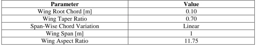
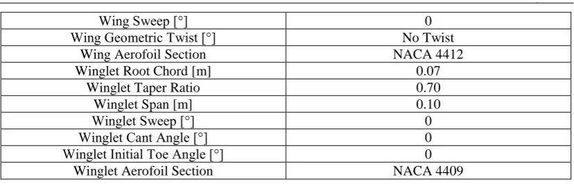
The geometrical characteristics of the chosen wing with winglets are presented in Table 1. As mentioned earlier in the paper, the focus is not on designing an efficient morphing-wing concept, and thus the baseline geometry is chosen without performing a multi-point design process, while the selected flight conditions are not based on investigating flight performance metrics for a specific UAV model.

Table 1 – Wing and Winglets Geometry Parameters

Parameter Value

Wing Root Chord [m] 0.10 Wing Taper Ratio 0.70 Span-Wise Chord Variation Linear

Wing Span [m] 1

Wing Sweep [°] 0 Wing Geometric Twist [°] No Twist

Wing Aerofoil Section NACA 4412 Winglet Root Chord [m] 0.07

Winglet Taper Ratio 0.70 Winglet Span [m] 0.10

Winglet Sweep [°] 0

Winglet Cant Angle [°] 0 Winglet Initial Toe Angle [°] 0

Winglet Aerofoil Section NACA 4409

The optimisations are performed at an airspeed of 10 m/s, for three angle of attack

values: -3°, 0° and 3°. The wing is modelled using 60 horseshoe vortices, clustered towards

the wing tips, while 20 horseshoe vortices are used for each winglet, clustered towards both the winglet tip and the junction with the wing tip. The lift curve slope and the zero-lift angle of attack for both wing and winglet aerofoils are taken from experimental data. The drag computations are limited to the induced drag component. For all optimisation runs, toe angles values are bounded between a lower limit of 𝜏𝑚𝑖𝑛 = −10° and an upper limit of

𝜏𝑚𝑎𝑥 = 10°. The trust-region algorithm used for solving the nonlinear system of the adjoint

simultaneous analysis and design approach is configured to stop when both the norm of the

linearized system residual ‖𝑭(𝒙𝑘)‖ and the norm of the solution change between two

consecutive steps ‖∆𝒙‖ become smaller than 10−10.

For the interior-point optimisation with adjoint-based gradient calculation, an objective function tolerance, a solution tolerance of and a constraints tolerance equal to 10−10 are used. All considered convergence criteria must be satisfied in order to accept the optimisation results. In addition, the convergence criteria for the iterative solution of the non-linear lifting line system of equations is set to 10−10, using the trust-region algorithm.

It must be noted that both optimisation approaches converge towards the same solution in terms of the design parameters (the two toe angles values), to an order of accuracy of two significant digits. Table 2 presents a comparison between the lift-to-drag ratio for the original design and for the optimised design, together with the toe angles values the morphing winglets take at each different angle of attack in order to achieve the indicated performance increase.

Table 2 – Performance Improvements Obtained Using Morphing Winglet Parameter

Original _𝑪𝑪𝑳

𝑫 Optimized

𝑪𝑳

𝑪𝑫 Winglet 1 Toe [°] Winglet 2 Toe [°] Angle of attack [°]

-3 19.07 21.10 -6.3208 6.3208

0 45.49 48.94 -5.9850 5.9850

3 42.31 44.55 -6.1178 6.1178

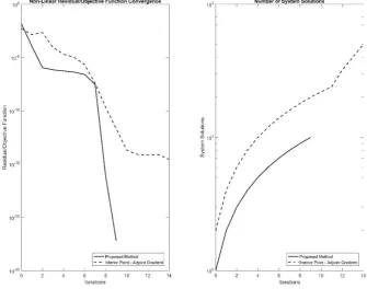
non-linear system residual ‖𝑭(𝒙𝑘)‖ or of the objective function 𝐽 together with the number

of system solutions required, as function of the iteration number, for the 3° angle of attack

optimisation case. The vertical axis of both plots uses a logarithmic scaling.

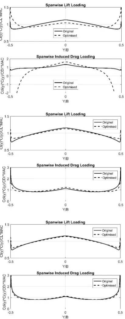
Fig. 1 – Comparison between the lift and induced drag span-wise loading between the original and optimized wing geometries, at angles of attack of -3 deg. (top two plots), 0 deg. (middle two plots) and

Fig. 2 – Convergence and computational effort of the two adjoint-based optimization approaches for the 3° angle of attack optimization case

Before discussing the relative performance of the algorithms, it must be kept in mind that the linearized system obtained for the Newton step of the trust-region method is a

system of (𝑁 + 𝑁 + 𝐷 + 𝐾) equations, while for the interior point optimisation method, the

aerodynamic model equations or the adjoint equations are only of size 𝑁.

Considering that the solution process of a linear system of equations requires 𝑂(𝑁3) operations (achievable when using the high-performance linear solvers implemented in MATLAB), the computational effort per linear system solution is higher with the proposed method.

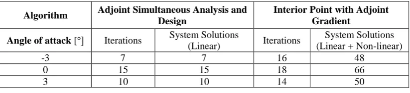
Table 3 summarises the number of iterations requires to achieve convergence and the total number of system solutions (either linear or non-linear) performed during the optimisation process, for both optimisation approaches and for all three optimisation cases.

In the case of the adjoint simultaneous method, one iteration means one linear system solution (the Newton step of equation (19)), but in the case of the interior point method, one iteration means one solution of the non-linear aerodynamics system (given by (36)) and one linear system solution (the adjoint equations (26)).

In addition, the number of system solutions (both non-linear and linear) per iteration is sometimes higher than two because of the two-step approach used by the interior point optimisation algorithm.

Table 3 – Comparison of Algorithm Performance

Algorithm Adjoint Simultaneous Analysis and Design

Interior Point with Adjoint Gradient

Angle of attack [°] Iterations System Solutions

(Linear) Iterations

System Solutions (Linear + Non-linear)

-3 7 7 16 48

0 15 15 18 66

3 10 10 14 50

As was mentioned, the non-linear lifting line system of equations is also solved using the trust-region algorithm.

However, because the Jacobian matrix is always non-singular and well-conditioned, the algorithm reduces to the simple Newton method.

A closer inspection of the solution process reveals that 10 iterations (comprising 10

linear system solutions) are sufficient to achieve the desired convergence criteria of 10−10.

Table 4 presents another comparison between the two optimisation approaches, but only in terms of total number of linear system solutions.

Table 4 – Comparison of Algorithm Performance (Only Linear System Solutions)

Algorithm Adjoint Simultaneous Analysis and Design Interior Point with Adjoint Gradient Angle of attack [°] Iterations System Solutions Iterations System Solutions

-3 7 7 16 264

0 15 15 18 366

3 10 10 14 275

It can be observed that the number of iterations required by the adjoint simultaneous method is slightly lower than the interior-point optimisation method.

The linear system obtained by applying the simultaneous method for this problem is a

system of (𝑁 + 𝑁 + 2 + 4) = (2𝑁 + 6) equations, with 𝑁 = 100.

Thus, one solution of the (2𝑁 + 6) linear system requires approximately 𝑂((2𝑁 +

6)3_{) ≈ 8 ∙ 𝑂(𝑁}3_{), thus 8 times more operations than one solution a 𝑁 size linear system.}

Looking over the results presented in Table 4, it is immediately seen that even with the significantly higher computational effort per linear system solution (due to the larger matrices), the overall number of operations required by the simultaneous method is much smaller compared to the gradient-based optimization algorithm using adjoint-determined gradient.

Thus, the adjoint-based simultaneous approach is more computationally efficient than the gradient-based optimisation approach for non-linear aerodynamic problems of interest having a high number of dependent variables and a relatively low number of design parameters.

This is the case for many problems of engineering interest, not only conceptual aerodynamic design using potential-flow methods.

6. CONCLUSIONS

The number of design parameters was much smaller compared to the number of dependent variables, as is the case for most problems of practical interest. Comparisons against the interior point algorithm using the traditional adjoint gradient calculation showed that the simultaneous approach was much more efficient in terms of the computational effort required, defined in terms of the total number of linear system solutions.

REFERENCES

[1] G. Carrier, D. Destarac, A. Dumont, M. Meheut, I. S. E. Din, J. Peter, S. B. Khelil, J. Brezillon and M. Pestana, Gradient-Based Aerodynamic Optimization With the elsA Software, 52nd AIAA Aerospace Sciences Meeting. AIAA Paper 2014-0568, 2014.

[2] A. Jameson, Aerodynamic Design via Control Theory. Journal of Scientific Computing, Vol. 3, No. 3, pp. 233-260, 1988.

[3] A. Jameson, Optimum Aerodynamic Design Using CFD and Control Theory, AIAA Paper 1995-1729, 1995. [4] K. Sermeus, K. Mohamed, E. Laurendeau and S. Nadarajah, Development of an Industrial Aerodynamic

Shape Optimization Strategy Using a Discrete Adjoint Method, 18th Annual Conference of the CFD Society of Canada, London, ON, Canada, 2010.

[5] S. Nadarajah and A. Jameson, A comparison of the continuous and discrete adjoint approach to automatic aerodynamic optimization, AIAA Paper 2000-0667, 2000.

[6] E. Fabiano, A. Mishra, D. Mavriplis and K. Mani, Time-Dependent Aero-acoustic Adjoint-based Shape Optimization of Helicopter Rotors in Forward Flight, 57th AIAA/ASCE/AHS/ASC Structures, Structural Dynamics, and Materials Conference, AIAA Paper 2016-1910, 2016.

[7] T. Blacha, M. M. Gregersen, M. Islam and H. Bensler, Application of the Adjoint Method for Vehicle Aerodynamic Optimization, SAE 2016 World Congress and Exhibition, SAE Technical Paper 2016-01-1615, 2016.

[8] G. K. W. Kenway and J. R. R. A. Martins, Multipoint High-Fidelity Aerostructural Optimization of a Transport Aircraft Configuration, Journal of Aircraft, Vol. 51, No. 1, pp. 144-160, 2014.

[9] J. Reuther, J. J. Alonso, M. J. Rimlinger and A. Jameson, Aerodynamic Shape Optimization of Supersonic Aircraft Configurations via an Adjoint Formulation on Distributed Memory Parallel Computers,

Computers & fluids, Vol. 28, No. 4, pp. 675-700, 1999.

[10] S. W. Funke, P. E. Farrell and M. D. Piggott, Tidal Turbine Array Optimisation Using the Adjoint Approach.

Renewable Energy, Vol. 63, pp. 658-673, 2014.

[11] S. A. Ragab, Shape Optimization of Surface Ships in Potential Flow Using an Adjoint Formulation, AIAA Journal, Vol. 42, No. 2, pp. 296-304, 2004.

[12] O. Polat and I. H. Tuncer, Aerodynamic Shape Optimization of Wind Turbine Blades Using a Parallel Genetic Algorithm. Procedia Engineering, Vol. 61, pp. 28-31, 2013.

[13] O. Şugar Gabor, A. Koreanschi, R. M. Botez, M. Mamou and Y. Mebarki, Numerical simulation and wind tunnel tests investigation and validation of a morphing wing-tip demonstrator aerodynamic performance,

Aerospace Science and Technology, Vol. 53, pp. 136-153, 2016.

[14] A. Koreanschi, O. Sugar-Gabor and R. M. Botez, Drag Optimisation of a Wing Equipped With a Morphing Upper Surface, The Aeronautical Journal, Vol. 120, No. 1225, pp. 473-493, 2016.

[15] O. Şugar Gabor, A. Koreanschi and R. M. Botez, Analysis of UAS-S4 Éhecatl Aerodynamic Performance Improvement Using Several Configurations of a Morphing Wing Technology, The Aeronautical Journal,

Vol. 120, No. 1231, pp. 1337-1364, 2016.

[16] D. G. Cacuci, Sensitivity and Uncertainty Analysis, Volume I: Theory, Boca Raton, FL, USA: CRC Press, ISBN 9781584881155, 2003.

[17] D. G. Cacuci, M. Ionescu-Bujor and I. M. Navon, Sensitivity and Uncertainty Analysis, Volume II: Applications to Large-Scale Systems, Boca Raton, FL, USA: CRC Press, 2005.

[18] R. H. Byrd, J. C. Gilbert and J. A Nocedal, Trust Region Method Based on Interior Point Techniques for Nonlinear Programming, Mathematical Programming, Vol. 89, No. 1, pp. 149-185, 2000.

[19] M. J. D. Powell, A FORTRAN Subroutine for Solving Systems of Nonlinear Algebraic Equations, Atomic Energy Research Establishment, Harwell (England), 1968.

[20] M. B. Giles and N. A. Pierce, An Introduction to the Adjoint Approach to Design, Flow,Turbulence and Combustion, Vol. 65, No. 3-4, pp. 393-415, 2000.

[22] R. A. Waltz, J. L. Morales, J. Nocedal and D. Orban, An Interior Algorithm for Nonlinear Optimization that Combines Line Search and Trust Region Steps, Mathematical Programming, Vol. 107, No. 3, pp. 391-408, 2006.

[23] W. F. Phillips and D. O. Snyder, Modern adaptation of Prandtl's classic lifting-line theory, Journal of Aircraft, Vol. 37, Issue 4, pp. 662-670, 2000.

[24] S. Barbarino, O. Bilgen, R. M. Ajaj, M. I. Friswell and D. J. Inman, A Review of Morphing Aircraft, Journal of Intelligent Material Systems and Structures, Vol. 22, Issue 9, pp. 823-877, 2011.

[25] L. Falcão, A. A. Gomes and A. Suleman, Aero-Structural Design Optimization of a Morphing Wingtip,

Journal of Intelligent Material Systems and Structures, Vol. 22, Issue 10, pp.1113-1124, 2011.