Performance Evaluation of Large Scaled Applications using Different Load Balancing Tactics in Cloud Computing

(1)

Performance Evaluation of Large Scaled

Applications using Different Load Balancing Tactics

in Cloud Computing

Minu Bala

Research Scholar Department of C.S. & I.T University of Jammu, J&K, India

Devanand, PhD

Professor

Department of C.S. & I.T University of Jammu, J&K, India

ABSTRACT

There is no doubt that workload distribution in cloud computing is one of the most important factors that regulates and dictates, directly or indirectly, its behavior and affects system performance. But geographical location of the datacenter and the user group is also an important factor that affects the overall performance of the system. This paper represents the performance analysis of three load balancing policies in combination with different broker policies for large-scaled applications using different infrastructural environments. The study has been made using CloudAnalyst: A CloudSim-based tool for modeling and analysis of large scale cloud computing environments. Experimental results reveal that large scaled software systems like FACEBOOK, TWITTER, ORKUT and e-commerce applications etc. can minimize their costs and improve service quality to the end users by making a right choice of service provider in the cloud market. The cloud service providers can also optimize their processing time by applying a best resource provisioning policy.

Keywords

Cloud Computing, IaaS, PaaS, SaaS, Load Balancing, Simulation.

1. INTRODUCTION

The rapid development of processing and storage technologies and the success of the internet has enabled the realization of new computing model called Cloud Computing[1], in which resources are provided as general utilities that can be leased and released by users through the internet in an on-demand fashion. Clouds offer services[2] that can be grouped into three categories: Software as a Service (SaaS), Platform as a Service (PaaS), and Infrastructure as a Service (IaaS).

Infrastructure as a Service: IaaS refers to on-demand

provisioning of infrastructural resources, usually in terms of VMs. The cloud owner who offers IaaS is called an IaaS provider. Examples of IaaS providers include Amazon EC2, GoGrid etc.

Platform as a Service: PaaS refers to providing platform layer

resources, including operating system support and software development frameworks. Examples of PaaS providers include Google App Engine, Microsoft Windows Azure etc.

Software as a Service: SaaS refers to providing on demand

applications over the Internet. Examples of SaaS providers include Google Apps, Facebook etc.

With the advancement of the Cloud, there are new possibilities opening up on how applications can be built on the Internet. On one hand there are the cloud service providers who are willing to provide large scaled computing infrastructure at a cheaper price which is often defined on usage, eliminating the high initial cost of setting up an application deployment environment, and provide the infrastructure services in a very flexible manner which the users can scale up or down at will. On the other hand there are large scaled software systems such as social networking sites and e-commerce applications gaining popularity today which can benefit greatly by using such cloud services to minimize costs and improve service quality to the end users.

2. FACTORS

AFFECTING

THE

PERFORMANCE OF LARGE SCALED

APPLICATIONS

2.1 Geographical Location

The geographical location of service provider matters a lot in the overall performance of large scaled applications on the cloud due to different network issues and the location of the user groups. Amazon EC2[3] provides the ability to place instances in multiple locations. It is currently available in nine regions: USEast (Northern Virginia), USWest (Oregon), USWest (Northern California), EU (Ireland), Asia Pacific (Singapore), Asia Pacific (Tokyo), Asia Pacific ( Sydney), South America (Sao Paulo) and AWS GorCloud. By launching instances of an application from different regions, failure of an application from single region can be protected.

2.2 Service Broker[4] Policy

The Service Broker entity is responsible for routing users’ requests coming from different user groups located at different geographical regions in globe to datacenters in cloud. The service broker policy can be of following types:

2.2.1 Closest Datacenter Policy

In this Policy, the Service Broker sends the request to closest datacenter in terms of Network Latency.

2.2.2 Performance Optimization Policy

(2)

2.2.3 Dynamic Configuration Policy

In this policy, the service broker is assigned an additional job of scaling the application deployment depending upon the load it is currently facing. It increases or decreases VMs dynamically in the datacenters according to the current processing times as compared against the best processing times ever achieved.

2.3 VM Load Balancing[5] Policy

The Datacenter Controller (DCC) is an entity which uses the VM allocation policy to route the user requests, received in the form of cloudlet, to the VM for processing.

2.3.1 Round Robin Policy

In Round Robin Policy, the requests of the clients are handled in a circular manner on first come first bases. The DCC directly interacts with the users’ requests and Load Balancer is the entity which assigns the load to the VMs. In this policy, the Load Balancer keeps record of all available VMs and also keeps track of next VM, to which next job is supposed to assign. As the new request comes from the user to DCC, it forwards request to the Load Balancer. The Load Balancer picks the next VM in circular order and assigns job in circular manner.

2.3.2 Throttled Policy

In this policy, each VM is assigned only one job at a time and another job can be assigned only when the current job has completed successfully. The Load Balancer entity maintains an index table of all VMs as well as their current states (Available or Busy). The client first makes a request to DCC for the allocation of appropriate VM and to perform the recommended job. The DCC queries the Load Balancer for allocation of the VM. The Load Balancer scans the index table from top to bottom until the first available VM is found. If it finds, returns the VM id to the DCC. Further, the DCC acknowledges Load Balancer about the new allocation and updates the index table of VM accordingly. On the other hand, if the Load Balancer doesn’t find any VM in the available state, it simply returns null. In this case DCC queues the request until the availability of any VM. When a VM suitably finishes processing the request, it sends a signal to the DCC about the completion of a job. The DCC further sends a signal to Load Balancer about the de-allocation of VM and updating its status in the index table. The DCC sees, if there is any queued request, sends it to the Load Balance for further processing.

2.3.3 Active Monitoring Policy

In this policy, load is equally distributed among all the VMs by actively monitoring the load on all the VMs. The Load Balancer maintains an index table of virtual machines and the number of allocations assigned to each virtual machine. Upon the arrival of a new request, the DCC queries the Load Balancer for allocation of new VM. The Load Balancer parses the index table from top until the least loaded VM is found. When it finds, it returns the VM id to the DCC. If there is more than one found, it uses first come first serve (FCFS) basis to choose the least loaded. Simultaneously, it also returns the VM id to the DCC. The DCC notifies the Load Balancer about the new allocation. It updates the index table by increasing the allocation count by 1 for that VM. When a VM suitably finishes processing the assigned request, it forwards a response to the DCC. On receiving the response it notifies the Load Balancer about the VM de-allocation which further updates the index table by decreasing the allocation count for that VM by 1.

3. PROPOSED STUDY

Quantifying the performance of different provisioning policies in a real cloud computing environment for different application models under variant conditions is extremely challenging due to the rigidity of the real infrastructure. Further, it is tedious and time consuming to reconfigure benchmarking parameters across massive scale cloud computing infrastructure over multiple test runs. So, the proposed study is to evaluate the performance of Large Scaled Application hosted at different geographical locations across the globe through simulations, using different resource provisioning policies.

4. SIMULATION

4.1 Simulation Tool

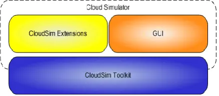
CloudAnalyst[6] is a GUI based simulator for modeling and analysis of large scaled applications. It is built on top of CloudSim toolkit, by extending CloudSim functionality with the introduction of concepts that model Internet and Internet Application behaviors.

[image:2.595.317.536.293.389.2]

Fig 1: CloudAnalyst built on top of CloudSim toolkit

Through GUI, its different components like Userbase, Internet, Service Broker Policy, Internet Cloudlet, Datacenter Controller and VM Load Balancing Policies can be configured differently for different cloud scenarios.

4.2 Simulation setup

[image:2.595.313.543.565.754.2]

Large Scaled Applications that could be benefited from the cloud computing are Social Networking Applications, e-Commerce Applications, Online Education Applications etc. For the present study, a Social Networking Application namely Facebook has been considered. The approximate users of Facebook[7] distributed across the globe as on 31-03-2012 are as under:

Table 1. Registered users of FB as on 31-03-2012

Geographic Region in order of

size Registered users

Europe 232,835,740

Asia 195,034,380

North America 173,284,940

South America 173284940

Central America 41,332,940

Africa 40,205,580

Middle East 20,247900

Oceania/Australia 13,597380

(3)

For the simulation purpose, the whole globe has been divided into six regions as R0, R1, R2, R3, R4 and R5. And grouping of registered users of FB as Userbases is done as under:

Table 2. Grouping of Regions & Userbases

Regions

Names of Geographic

Regions

Userbase

Registered users

R2 Europe UB3 232835740

R3 Asia, Middle East

UB4

215282280

R0

North America, Central America,

Caribbean,the

UB1

220973200

R1 South America UB2 112531100

R4 Africa UB5 40205580

[image:3.595.315.542.330.527.2]

R5 Oceania/Australia UB6 13,597380 In order to bring the simulation framework more close to the real environment, the network behavior of the simulation model as been configured as per the network characteristics of Amazon EC2. It has been assumed that only 5% of the registered users remain online during peak hours and 1/10th of peak hour users will remain online during off-peak hours. It is further assumed that each user makes a new request after every 5 minutes when online. The following parameters have kept fixed for all simulation scenarios.

Table 3. Parameters fixed for simulations

Parameter Value

Simulation duration 60 min.

Requests per user per hr. 12

Data Size per request per hr. 100 bytes No. of Hosts (Each having 4

processors) 40

User Grouping factor in

Userbases 10000

Request Grouping factor in

Datacenters 1000

Executable instruction length

per request 500 bytes

4.2.1 Scenario 1 Setup & Observations

In scenario 1, simulation runs have been made for one datacenter, by changing its location one by one to each geographical region, for three Service Broker Policies (Closet Data Center, Optimal Response Time and Dynamic Configuration) each in combination with three VM Load Balancing Policies (ESCE, RR, and Throttling) one by one. The observations made during all simulation runs are depicted in the following three tables.

Table 4. Overall Response Time of a datacenter using ESCE Load Balancing Policy

Regions

Closest Data Center

Policy

Optimal Response Time Policy

Dynamic Configuration

Policy

R0 97187 97308 96674

R1 96972 96861 96583

R2 97250 97682 96623

R3 97736 97410 97170

R4 97099.7 97084.8 96409

R5 97289 97215 96597

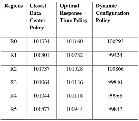
Table 5. Overall Response Time of a datacenter using Round Robin Load Balancing Policy

Regions Closest

Data Center Policy

Optimal Response Time Policy

Dynamic Configuration Policy

R0 101534 101160 100293

R1 100801 100782 99424

R2 101737 101928 100866

R3 101064 101136 99840

R4 101344 101118 99965

[image:3.595.53.283.406.631.2]

R5 100877 100944 99847

Table 6. Overall Response Time of a datacenter using Throttled Load Balancing Policy

Regions

Closest Data Center

Policy

Optimal Response

Time Policy

Dynamic Configuration Policy

R0 14063 14046 14057

R1 14229 14219 14211

R2 14081 14079 14052

R3 14189 14187 14172

R4 14341 14338 14319

[image:3.595.313.542.565.760.2]

(4)

4.2.2 Scenario 2 Setup & Observations

[image:4.595.316.540.115.302.2]

In scenario 2, simulation runs have been made for two identical datacenters, by changing the location each datacenter one by one according to the combinations as (R0 & R2), (R1 & R2) and (R1 & R3), for three Service Broker Policies (Closet Data Center, Optimal Response Time and Dynamic Configuration) each in combination with three VM Load Balancing Policies (ESCE, RR, and Throttling) one by one. The observations made during all simulation runs are depicted in the following three tables:

Table 7. Overall Response Time of two datacenters using ESCE Load Balancing Policy

Regions

Closest Data Center Policy

Optimal Response Time Policy

Dynamic Configuration

Policy

R0 & R2 57823.3 56307.73 55704.27

R1 & R2 57815.65 54592.58 55697.57

[image:4.595.315.540.118.506.2]

R1 & R3 56468.52 53461.12 54498.55

Table 8. Overall Response Time of two datacenters using Round Robin Load Balancing Policy

Table 9. Overall Response Time of two datacenters using Throttled Load Balancing Policy

Regions

Policy

R0 & R2 10177.81 9532.12 10157.8

R1 & R2 10203.52 9638.43 10179.89

R1 & R3 10097.06 9323.4 11205.87

4.3 Graphical Representation and Analysis

[image:4.595.53.277.208.361.2]

The graphical representation of experimental observations obtained in scenario 1 are depicted in Fig. 2, 3, 4 & 5.

Fig.2 Overall Response Time of a Datacenter at different regions using different Policies at Broker Level and

[image:4.595.318.537.333.506.2]

Active Monitoring LB Policy at VM level

Round Robin LB Policy at VM level

Throttled LB Policy at VM level

95500 96000 96500 97000 97500 98000

R0 R1 R2 R3 R4 R5

Re gions

O

v

e

r

a

ll

R

e

sp

o

n

se

T

im

e

(

i

n

m

se

c

.) Closest

Data Center Policy

Optimal Response T ime Policy Dynamic Configurati on Policy

98000 98500 99000 99500 100000 100500 101000 101500 102000 102500

R0 R1 R2 R3 R4 R5

Regions

R

e

s

p

o

n

s

e

T

im

e

(

in

m

s

e

c

.)

Dynamic Configuration Policy

13850 13900 13950 14000 14050 14100 14150 14200 14250 14300 14350 14400

R0 R1 R2 R3 R4 R5

Regions

R

e

s

p

o

n

s

e

T

im

e

(

i

n

m

s

e

c

) _{Closest Data}

Center Policy

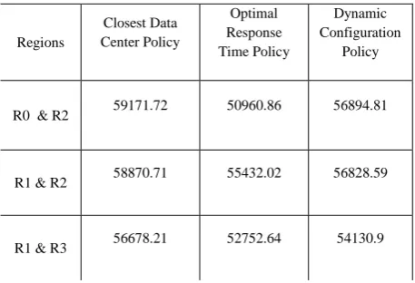
Dynamic Configuration Policy Regions

Policy

R0 & R2 59171.72 50960.86 56894.81

R1 & R2 58870.71 55432.02 56828.59

[image:4.595.53.282.401.557.2] [image:4.595.320.532.543.719.2]

(5)

[image:5.595.63.272.71.294.2]

Fig. 5 Overall Response Time of a Datacenter at different regions using Dynamic Configuration Policy at Broker

Level and different LB Policies at VM Level

[image:5.595.319.539.74.230.2]

The experimental results depicted in Fig. 2, Fig. 3 and Fig. 4 reveals that the overall response time of a datacenter changes with the change in the geographical location of datacenter. It is better when the service broker policy is Dynamic than other two policies (Closest Data Center, Optimal Response Time) using any of the three VM Load Balancing Policies considered in the experimentation. The result analysis in Fig. 5 reveals that out of the three considered VM Load Balancing Policies, the overall response time of the Datacenter is better in case of Throttled Load balancing Policy. And the results are better when the geographical location of the datacenter is Region R2 than other five regions.

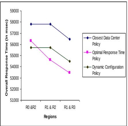
Fig.6 Overall Response Time of two Datacenters located at two different regions using different policies at broker

[image:5.595.316.539.276.449.2]

level and Active Monitoring LB Policy at VM level

level and Round Robin LB Policy at VM level

level and Throttled LB Policy at VM level

Fig.9 Overall Response Time of two Datacenters located at two different regions using Optimize Response Time

Policy at broker level and different LB Policies at VM Level 0 20000 40000 60000 80000 100000 120000

1 2 3 4 5 6

Regions R e s p o n s e T im e ( in m s e c .) Active Monitoring RR Throttled 51000 52000 53000 54000 55000 56000 57000 58000 59000

R0 &R2 R1 & R2 R1 & R3

Regions O v e r a ll R e s p o n s e T im e ( in m s e c )

Optimal Response Time Policy Dynamic Configuration Policy 46000 48000 50000 52000 54000 56000 58000 60000

R0 & R2 R1 &R2 R1 & R3

Regions O v e ra ll R e s p o n s e T im e ( in m s e c )

Closest Data Center Policy Optimal Response Time Policy Dynamic Configuration Policy 0 2000 4000 6000 8000 10000 12000

R0 & R2 R1 & R2 R1 & R3

Regions O v e ra ll R e s p o n s e T im e ( in m s e c .)

Closest Data Center Policy Optimal Response Time Policy Dynamic Configuration Policy 0 10000 20000 30000 40000 50000 60000

R0 & R2 R1 & R2 R1 & R3

Regions O v e r a ll R e s p o n s e T im e ( in m s e c .)

Active Monitoring LB Policy

Round Robin LB Policy

[image:5.595.56.279.480.698.2] [image:5.595.319.538.499.699.2]

(6)

5. CONCLUSION

Besides service broker policy and VM load balancing policy, the geographical location of the datacenter where a large scale application is hosted and the geographical location of its end users, affect the overall performance of the system. The choice of datacenter’s location according to location of its maximum end users improves the results. Thus the overall response time of the application to the end users can be optimized by making a right combination of the above mentioned elements. Moreover such type of simulation work helps to generate a valuable insight for Application Designers in identifying the optimal configuration for their application.

6. REFERENCES

[1] Luis M. Vaquero, Luis Rodero-Merino , Juan Caceres, Maik Lindner, ”A Break in the Clouds: Towards a Cloud Definition”, ACM SIGCOMM Computer Communication Review, Volume 39, Number 1, Pages 50-55, Jan. 2009.

[2] Rajkumar Buyya, Chee Shin Yeo, Srikumar Venugopal, James Broberg, and Ivona Brandic, “Cloud Computing and Emerging IT Platforms: Vision, Hype, and Reality for Delivering Computing as the 5th Utility, Future

Generation Computer Systems”, Volume 25, Number 6, Pages: 599-616, ISSN: 0167-739X, Elsevier Science, Amsterdam, The Netherlands, June 2009.

[3] www.aws.amazon.com/ec2

[4] R. Buyya, R. Ranjan, and R. N. Calheiros, “Modeling And Simulation Of Scalable Cloud Computing Environments And The Cloudsim Toolkit: Challenges And Opportunities,” Proc. Of The 7th High Performance Computing and Simulation Conference (HPCS 09), IEEE Computer Society, June 2009.

[5] Jasmin James and Dr. Bhupendra Verma, “Efficient VM load balancing algorithm for a cloud computing environment”, International Journal on Computer Science and Engineering (IJCSE), 09 Sep 2012. [6] Bhathiya Wickremasinghe, “CloudAnalyst: A CloudSim

based Tool for Modeling and Analysis of Large Scale Cloud Computing Environments” MEDC project report, 433-659 Distributed Computing project, CSSE department., University of Melbourne, 2009.